R.L. Parker, The magnetotelluric inverse problem - MTNet

THE MAGNETOTELLURIC INVERSE PROBLEM 

ROBERTL. PARKER 

Institute of Geophysics and Planetary Physics, Scripps Institution of Oceanography, University of 

Cali]brnia, San Diego, La Jolla, CA 92093, U.S.A. 

Abstract. The magnetotelluric inverse problem is reviewed, addressing the following mathematical 

questions: (a) Existence of solutions: A satisfactory theory is now available to determine whether or not a 

given finite collection of response data is consistent with any one-dimensional conductivity profile. (b) 

Uniqueness: With practical data, consisting of a finite set of imprecise observations, infinitely many solutions 

exist if one does. (c) Construction: Several numerically stable procedures have been given which it can be 

proved will construct a conductivity profile in accord with incomplete data, whenever a solution exists. (d) 

Inference: No sound mathematical theory has yet been developed enabling us to draw firm, geophysically 

useful conclusions about the complete class of satisfactory models. 

Examples illustrating these ideas are given, based in the main on the COPROD data series. 

I. Introduction 

This paper is a review of progress in the study of the magnetotelluric inverse problem 

for a very simple physical system - an electrically conducting halfspace in which the 

conductivity cr varies only with depth and is isotropic. Despite the simplicity of the 

mathematical model and of the governing differential equations, the relation between 

the observed quantities and the unknown conductivity profile is nonlinear; this fact 

makes the problem difficult and there are still some aspects of it that are far from 

understood. The usefulness of the model can best be judged by the large number of 

papers in the geophysical literature relying upon it for interpretational purposes and by 

the almost equally large number devoted to advancing the associated theory. 

Let us first define the geophysical system more precisely and introduce some 

terminology. Electromagnetic induction takes place in the conducting halfspace driven 

by a periodic horizontal magnetic field, varying in time like e ~'. The electric and 

magnetic fields found at the surface of the conductor are not independent of each other: 

the electric field is also horizontal and perpendicular to the magnetic field; its 

magnitude and phase relative to the magnetic field depend upon the conductivity 

below, which is of course the basis of the magnetotelluric method. For convenience we 

erect a Cartesian coordinate system with origin at the surface, z downward and x 

parallel to the magnetic field. Then using Weidelt's (1972) definition we introduce a 

complex response given by 

c = - E:r r. 

This complex number varies with the frequency of the source field. Natural elec- 

tromagnetic fields contain energy at all frequencies; if these fields are measured we may 

make estimates of c by Fourier analysis of the observed time series of E~ and By. 

Practical considerations limit these estimates to a finite collection of responses at a 

number of distinct frequencies: 

Geophysical Surveys 6 (1983) 5-25.0046-5763/83/0061-0005503.15. 

9 1983 by D. Reidel Publishing Company.

6 ROBERT L, PARKER 

cj = c(coj), j = 1, 2 .... N. 

More conventionally in the geophysical literature observations are represented in 

terms of the apparent resistivity p, and phase ~p: 

C = (pa/l~Oco)l/2e i(4)-~/2). 

A uniform halfspace exhibits a constant value of Pa equal to the resistivity of the 

medium and Re c is twice the skin depth. When the conductivity varies with depth, this 

allows a rudimentary interpretation of p, to be made as the approximate resistivity 

averaged over the penetration scale of the energy at the frequency in question. Inside 

the medium the electric field E (we drop the subscript x) obeys the differential equation 

dZE 

2 - ico ,o (Z)E. (1) 

A boundary condition is supplied to insure that no energy is provided to the system 

from below: we say E ~ 0 as z ~ ~c; alternatively the vertical extent of the conductor 

may be made finite and then E = 0 at the bottom. From Maxwell's equations it follows 

that 

c = 0. (2) 

Our task then is to determine whatever we can about o in (1) from the observations ofc 

and its relation to E in (2). As I suggested in a general review (Parker, 1977a), inverse 

problems like this one raise a number of mathematical issues, which we consider in 

turn. 

2. Existence of Solutions 

We should first decide whether a given data set is compatible with the mathematical 

model. The simplifications of the model, such as the uniformity of the source field and 

the lack of lateral variations in a, are such that we ought not be surprised when the 

measurements cannot be reconciled with any one-dimensional profile. The question of 

existence is whether there is any model at all which can adequately satisfy the 

observations. This raises the question of what is meant by agreement between the 

predictions of a model and the data. The easiest case to analyze is the idealized one in 

which the data are supposed to be exactly known: we have a set of complex numbers cl, 

C2, ..., C N or, in this case precisely equivalently, pairs (Pa, ~P)I, (P,, ~P)Z, " ", (Pa, ~b)N 

corresponding to frequencies co~, co2, ---, con. Weidelt (1972) gives 19 inequalities 

involving the real and imaginary parts of c, which every realizable data set must obey. (I 

should say at this point that Weidelt's paper, written over ten years ago, is a landmark 

in the study of the inverse magnetotelluric problem; it touches on all the important 

issues; it is rightly the most widely quoted paper in the literature and has had a 

profound influence on the subject.) Most of Weidelt's relations involve derivatives of c

THE MAGNETOTELLURIC INVERSE PROBLEM 7 

which cannot be obtained exactly from discrete data; nonetheless, bounds on dc/d02 

and dZc/dco 2 can be obtained. The basis of Weidelt's inequality constraints is the fact 

that c must always be expressible as an integral over a nondecreasing real function a(2)" 

c(02) = f fyT da(2) . (3) 

0 

This is a Stieltjes integral, which for continuously increasing functions may be 

interpreted as 

co 

c(02) = f 

da d2 

d2 2 + i02 

i/ 

0 

However, for many conductivity profiles the function a(2) exhibits jumps, which 

contribute terms of the form 

Ao n 

2. + i02' 

where Aa, > 0 is the magnitude of the jump in a and 2, is the value of 2 where it is 

located. The function a(2) is called the spectral function for Equation (2) and plays a 

central role in the theory of that differential equation. The points 2 at which a(2) 

increases correspond to eigenffequencies i2 of the system under the surface boundary 

condition dE/dz = O. 

Weidelt (1972) and several others (e.g. Bailey, 1970; Fischer and Schnegg, 1980) 

have discussed relationships between the real and imaginary parts of c and between pa 

and 4). In a genuine response, these pairs of functions are not independent so that, for 

example: 

~b(02) _ n 02 fin [p.(02')1 ,do)' 

4 L J02 i -02 TM 

0 

Such connections, called dispersion relations, result from the fact that c(02) has no zeros 

or singularities below the real axis in the complex 02 plane, when c is considered as a 

function of complex frequency. Unfortunately, such relations are weak constraints on 

the data for two reasons. First, they require knowledge of the response function for all 

02, not just at 021,022 . . . . . (.ON; this is an unrealistic demand. Second, they are satisfied by 

any function that dies away fast enough at infinity and whose singularities and zeros lie 

above the real 02 axis. This far less restrictive than Equation (3), which forces the zeros 

and singularities onto the positive imaginary 02 axis. 

The conditions discussed so far are only necessary conditions for a solution to exist 

for the one-dimensional inverse problem. This means there are functions satisfying 

them that are not valid responses. For example, 

1-i 1+i02 

1 + i02 - o) 2 

satisfies the dispersion relations for any positive ~; in addition, if 0 < c~ < 0.048 033,

8 ROBERT L. PARKER 

satiesfies all Weidelt's inequalities as well. But ~ has poles at co = (1 ix/3)/2 which are 

inadmissible in a true one-dimensional response. 

The author (Parker, 1980) has provided a complete theory for the existence of 

solutions based essentially on the representation (3). If the sampled responses are 

substituted into (3) we obtain 

f da(2) 

c j= 2+icoj' j=l'2 ..... N, (4) 

0 

where we may recall a(2) is a nondecreasing real function. These constraints can be 

viewed as requiring the consistency of a semi-infinite linear programming problem for 

the unknown a. I show that if there are any solutions to (4) at all there must be one in 

which a(2) consists of a function that is constant except at J points of discontinuity, 

where the function jumps and J ~< 2N. To realize the test practically requires the 

approximation of the integral by a sum, and the application of standard linear 

programming algorithms. The convergence of a sequence of matrix approximations to 

the true integral can be established mathematically and in many numerical tests 

performed by the author extremely rapid covergence is observed. If a given collection of 

data cj passes the test then solutions ~ do exist, provided we agree to admit perfectly 

thin conducting sheets of the type introduced by Price (1949); this is because the 

conductivities corresponding to spectral functions a(2) that increase at only a finite 

number of points consist of a series of delta functions: 

J 

o(z)= Z (5) 

k=l 

The class of models in this form is called D +. Thus the test is a necessary and sufficient 

one for solutions to exist. 

It may be disappointing that the nesessary an d sufficient condition takes the form of a 

fairly complex calculation and cannot be summed up in a succinct formula. However, 

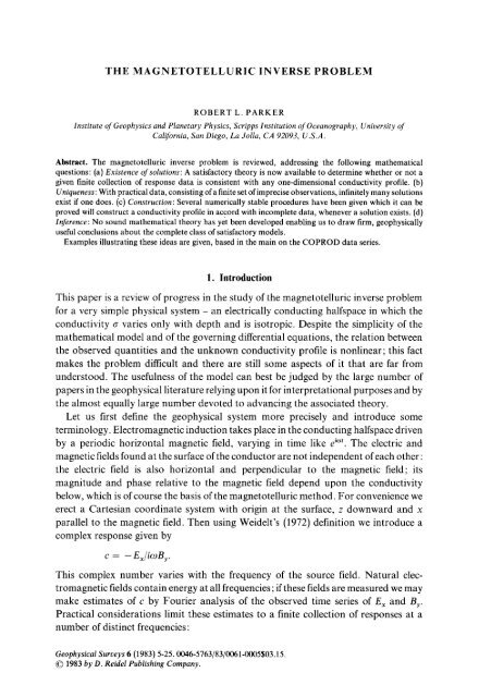
the condition is subtle, as the following example illustrates. Figure la shows a simple 

model made up of uniform layers, terminated by a uniform half-space; Figure lb shows 

the corresponding complex response c and the fifteen frequencies at which the response 

is sampled for a test. (The model gives a reasonable fit to the COPROD data set and the 

frequencies are those appropriate to that series; we shall discuss the COPROD 

observations more fully in a moment.) I performed the following numerical experiment. 

Each of the numbers was rounded to four significant figures. The consistency of this 

slightly perturbed set was tested and I found that the conditions (4) could be satisfied 

only to about four figures. If the accuracy of the responses was improved the fit also 

improved, until at around seven significant figures no further improvement could be 

obtained; this plateau is probably a result of the finite accuracy of the computer 

arithmetic (some parts of the calculation are performed in single precision on a 32-bit 

computer). We may conclude that no one-dimensional model can exactly satisfy the 

responses that had been rounded to four figures. This and similar numerical experi-

Fig. 1. 

~, 10 ~ 

m,~ 10-1 

b 

10-2 

~ 10_3 

0) 

i/] 

o 

0 

O) 

f:h 

~ 10-4 

200 

100 

-100 

-200 

0 

THE MAGNETOTELLUR1C INVERSE PROBLEM 9 

(a) 

0 100 

I I I 

200 300 400 

Depth z (km) 

I I 

500 600 

(b) 

I I I I [111 I I I I [ I III I 

10-z 10-1 

Radian frequency w (s -1) 

(a) A simple uniform slab model. (b) Theoretical complex response c of the model; the fifteen 

sampling frequencies are the same as those in the COPROD data series. 

Conductivity Model of Figure la 

Conductivity (S/m) Thickness (km) 

0.0 13.426 

0.010857 36.288 

0.002275 167.145 

0.00049519 179.28 

0.1 infinity 

Complex response c of Figure lb 

Radian freq (i/s) Real c (km) Imagc (kin) 

0.2205 25.759 254 - 12.496 435 

0.1632 27.239246 -14.736553 

0.1205 28.896709 - 17.704082 

0.0891 2 30.874535 -21.559002 

0.0657 9 33.299 438 - 26.456165 

0.0486 7 36.165 070 - 32.558 403 

0.0359 7 39.518 440 - 40.395 363 

0.0265 9 43.619 400 - 50.708 069 

0.0196 5 49.232 292 - 64.408 722 

0.0145 2 57.726 242 - 82.235 886 

0.01074 71.072678 - 104.31247 

0.0079 35 91.884 109 - 129.891 78 

0.005866 122.33662 -156.17935 

0.0043 35 163.057 92 - 178.816 59 

0.0032 04 211.345 70 - 193.087 46


ments suggest the virtual impossibility of ever obtaining an exact fit to experimental 

data. 

We are brought back to the question of what is meant precisely when we ask for a 

satisfactory agreement between theory and observation; clearly an exact fit is 

unreasonably demanding. The answer depends of course on the uncertainties ascribed 

to the data. It is important to remember that the actual quantities recorded are the 

horizontal components of electric and magnetic fields and that these time series must be 

processed to yield a magnetotelluric response. The uncertainties depend on the nature 

of the noise in the signals and on the way in which the time series are manipulated. If 

most of the noise is in one of the two signals (say the electric field is contaminated by 

random fields not due to telluric induction), then a standard theory (e.g. Bendat and 

Piersol, 1971 ) exists for optimal estimation of the transfer function between E and B; 

after its application one finds that at each frequency the response c consists of 

uncorrelated real and imaginary parts with equal variances, the value of the variance 

depending on the coherence between the signals. Furthermore, the probability function 

for lc - c72 follows an F distribution curve with parameters that depend on the way in 

which the data are grouped. For reasonable choices of grouping the F distribution is 

well approximated by a Gaussian function. Unfortunately, it seems unlikely that the 

conditions for this theory apply to magnetotelluric observations and no entirely 

satisfactory theory has been developed as an alternative; in any event there is no 

generally agreed upon method for determining responses from field data. The situation 

is complicated by the fact that an impedance tensor must be estimated rather than a 

scalar. Bentley's (1973) study is widely quoted, but it should be noticed that his log- 

normal distribution for p, was put forward entirely empirically. It seems to me that 

there is no good reason to believe that Pa and q~ are the statistically appropriate pair of 

variables to use; in fact, we expect that the real and imaginary parts of the transfer 

function (and hence of c) will have a simpler statistical description than that ofpa and 4. 

In the absence of a generally accepted theory for the statistics of the data, authors 

have felt free to pick their own criteria for acceptability of a fit, often without any 

theoretical justification whatever. Hobbs (1982) writes: 'MT analysts are notoriously 

optimistic in believing the significance of the errors accompanying their data, the result 

being that in some cases no model exists whose response fits...'; he uses this assertion 

as an argument for raising experimental error estimates if he is unable to find a suitable 

model! Fischer et al. (1981 ) adopt a measure of misfit consisting of the sum of squares of 

differences in q~ and in in p,, each quadratic term weighted by the inverse confidence 

interval (not the square of the interval as traditional practice would suggest). They also 

propose omitting a term form the sum whenever it is less than some arbitrary amount. 

Similar misfit measures have been used by many other authors (e.g. Larsen, 1981; 

Khachay, 1978; Fischer and Le Quang, 1981) presumably all motivated by Bentley's 

suggestion; weighting of the quadratic terms in the sum is often omitted. Another 

definition of a satisfactory model is given by Jones and Hutton (1979); they accept a 

conductivity profile (calling it 'acceptable at the 75 ~ level' !) if more than 75 ~ of the 

theoretical responses lie within the 95 ~ confidence intervals of p, and q~.

THE MAGNETOTELLURIC INVERSE PROBLEM ] 1 

Most of the above treatments can be characterized as follows. The collection of 

measured responses may be represented as an element D e E 2u, where E 2N is a normed 

2N-dimensional linear vector space; the predictions of the model are | e E 2N. The 

disagreement between D and O, the misfit, is measured by the norm of EZN; if 

II O - DII < T, 

where Tis a tolerance, the model fits the data. The trouble with many of the above misfit 

measures is that there is no apparent rational basis for the choice of T that separates 

good models from bad ones. The following old fashioned approach seems quite 

reasonable. We set up the hypothesis that the true profile is the model under 

consideration and that the disagreement between model responses and observation are 

caused by the randomness in the data estimates. It is always possible to make some 

assessment of var D j, the variance of the j-th observation; the crudest approach is to 

calculate the scatter obtained when the field time series are broken into a number of 

independent records and Dj is obtained from each. Then we can use a 2-norm in E 2N; let 

x 2 = II O - oii 2 = ~(Oj - Dj)2/varDj. 

J 

We must now calculate the probability that Z 2 would reach or exceed the observed level 

by chance; if the probability is too low (say less than 0.05) we must reject the model. 

When Dj are independent Gaussian random variances the probability is distributed as 

Z 2, or for large enough numbers of data, approximately normally. With more exotic 

distributions for Dj approximate confidence levels can be found by the central limit 

theorem. The number of 'degrees of freedom' is 2N, the number of independent data in 

the sum. This treatment may be rough, particularly in view of the uncertainties in var D~ 

or the possible lack of statistical independence of the variables D j, however the choice of 

T is founded in some sort of statistical model in contrast to most of those in the 

geophysical literature. The problem of existence is reduced to that of finding the model 

with Z 2 as small as possible; if this model is rejected so will every other model and we 

must conclude that there is no one-dimensional profile capable of reproducing the data. 

The criterion suggested here runs the risk of a type II statistical error (accepting the 

existence of a one-dimensional model when in fact none exists) because we have not 

accounted for the fact that the predictions O~ are not independent of the data. 

Nonetheless, 1 have found it to be far less generous than the ad hoc criteria currently 

fashionable. 

With these ideas it is not hard to adapt the existence theory developed for exact data 

to the case of noisy data (Parker and Whaler, 1982). Now we minimize 

o| 

r dat / 21 

j=l cj -- j 2 + ir ~ Sj 

(6) 

0 

over all nondecreasing spectral functions a(~). This is a semi-infinite quadratic 

programming problem which can be solved by standard methods. It is found that, as 

with exact data, there is always a spectral function a(2) minimizing (6) which has only a


Fig. 2. 

v 

0 

O 

C.9 

101 

10 o 

10-1 

10-2 I I I I I I I I 

0 100 200 300 400 

Depth z (kin) 

Delta function solution with smallest misfit in the sense ofz 2 for the experimental COPROD data 

set (the fifteen well-estimated responses); Z?~in = 33.7. 

Model of Figure 2 

Depth (km) Conductance (kS) 

25.263 0,352 77 

91.043 0,356 03 

387.80 2.287 5 

finite number of jumps and is otherwise constant. This means that (1) has only a finite 

number of eigenvalues, which can happen only if a is in the form of (5), i.e. a consists of a 

sum of delta functions. No other model 'can have a Z 2 smaller than the delta-function 

model that fits the data best. 

As an illustration let us turn to the data set of the COPROD study organised by A. G. 

Jones. This set has been the subject of many investigations (e.g. Jones and Hutton, 

1979; Larsen, 1981; Fischer and LeQuang, 1981; Hobbs, 1982; Parker, 1982). I 

followed the assumption that p, and r are uncorrelated and calculated an approximate 

standard deviation for them by dividing the given confidence interval by 3.92, the 

number appropriate for a Gaussian distribution. In (6) I included a modification to 

account for the covariance in c introduced by making p, and r uncorrelated variables 

with unequal variances. For the 15 well estimated respoiases, the minimum Z 2 = 33.7, 

which is easily within the 95 ~ value of 43.8; there is no doubt that one-dimensional 

profiles exist in accord with these data, because many investigators have already found 

them. The best fitting model has not been published before; it appears in Figure 2. 

When all 23 responses of the COPROD data set are included the smallest Z 2 increases 

to 1.66 104, which causes us to reject the possibility of a one-dimensional model with 

more than 99.9 ~ certainty.


It is possible to minimize other misfit measures in (6) in place of the simple quadratic 

functional; then a nonlinear optimization scheme which applies the positivity 

constraints on da(2) must be used. As described in Section 4, Khachay (1978) has done 

something quite similar to this. Thus, through the use of the spectral function 

representation of a response, the problem of determining whether or not any one- 

dimensional models exist satisfying a practical data set has been solved. Best-fitting 

models are however not geophysically plausible because they consist of a series of delta- 

functions in conductivity. 

3. Uniqueness 

Suppose it has been decided that a given collection of response data is compatible with a 

one-dimensional conductivity profile; we may ask whether only one such profile fits the 

data, or whether more than one model can accomplish this feat. The answer depends on 

the type of data available. It has been long known (Tichonov, 1965; Bailey, 1970) that 

when the given responses are exact at all frequencies a solution, if it exists at all, is 

unique (at least, for a class of sufficiently smooth models). Obviously, since Pa and ~ are 

inter-related, complete knowledge Ofpa alone yields a unique solution too (as does the 

real part of c). Suppose c (or pa) is known precisely for all co with col < co < o92; since c is 

an analytic function of co with singularities on the positive imaginary axis, it can be 

analytically continued into the complex co plane and, more specifically, calculated 

everywhere on the real axis. Hence complete knowledge of c on any open interval is 

equivalent to knowledge of c at all frequencies, and therefore only one model can fit 

exact data given everywhere in a finite frequency band. Less well known perhaps is the 

fact that c (or p,) can be unambiguously reconstructed from an infinite set of samples 

taken at evenly spaced frequencies: coo, coo + Aco, coo + 2Aco ..... for any coo, Aco > 0 

(see Lanczos Chapter 1, 1961). Again a solution is unique if its satisfies observations at 

all these frequencies. 

Every one of the above cases requires knowledge of c or p, at infinitely many 

frequencies, something which is, practically speaking, impossible. Because the un- 

known a is a function, we should not expect it to be uniquely defined by a finite number 

of constraints even when these are given precisely. Certaintly we know from our 

discussion of existence that, if an ordinary (say piece-wise continuous) model satisfies 

the data, then there is another solution in terms of data functions. Figure 3 illustrates 

this; synthetic data consisting of the fifteen complex responses of Figure lb are fitted 

very precisely (to about 4 parts in 10 6) by the delta function solution shown; recall that 

these data were generated from the model in Figure la. The profiles of Figures la and 3 

are two completely different conductivities, both satisfying a finite data set essentially 

exactly. In fact it is possible to find certain finite data sets that can be satisfied exactly by 

only one model (Parker, 1980), but this situation must be regarded as anomalous. 

The case of imprecise observations is trivial. If any model exists satisfying 

II | - DII < T, 

then surely so do infinitely many others: the solution cannot be unique.


o 

o 

c9 

101 

10 o 

10-1 

IN i 1 i i i 

. -2 0 100 200 300 400 500 600 

Depth 

(km) 

Fig. 3. A delta function model satisfying the synthetic responses of Figure lb. 

Model of Figure 3 

Depth (km) Conductance (kS) 

16.075 0.085 962 

29.168 0.195 70 

50.269 0.196 32 

114.34 0.161 27 

181.56 0.16747 

399.96 1.574 7 

426.62 2.943 7 

460.47 3.663 1 

408.51 4.349 0 

553.40 7.021 0 

638.96 10.094 

4. Construction 

We come now to the question that occupies that attention of the vast majority of 

geophysicists working on the magnetotelluric inverse problem: how can we find an 

example of a conductivity profile that fits our observations, provided of course that 

such a model exists? Until very recently there was no satisfactory existence theory and 

so the failure of a specific algorithm could be attributed to the inadequacy of the data 

rather than to any weakness in the modeling technique. Lack of uniqueness of the 

solutions means that there is a certain arbitrariness about the model obtained; it also 

sheds doubt on the usefulness of any individual profile for geophysical interpretation. 

Jones (1982) writes '... it is axiomatic in geophysical data interpretation to find the 

simplest model - or models that satisfies the observed response...' This widely held 

belief is surely reasonable, but it offers little help in suggesting a way out of the difficulty 

of arbitrariness because the idea of simplicity is quite subjective. In practice there are

THE MAGNETOTELLURIC INVERSE PROBLEM l 5 

two schools of thought on the matter: one regards solutions consisting of a small 

number of uniform layers separated by discontinuities as simple models; the other 

elects smoothly varying functions with small gradients to be the preferred class. The 

discontinuous models may well be appropriate in the upper crust where large 

conductivity contrasts may be found at the contact between geologically different units; 

deeper in the Earth phase changes could cause sudden jumps in conductivity too, but it 

seems for some depth ranges more likely that smoothly increasing temperature will 

determine the behavior of ~r and then a smooth function would seem to be the proper 

archetype. 

Let us first review the discontinuous solutions, which have been the subject of 

intensive study (e.g. Jupp and Vozoff, 1975; Shoham et al., 1978; Benvenuti and 

Guzzon, 1980; Larsen, 1981; Fischer and Le Quang, 1981). In these and other 

investigations the idea of simplicity is enforced by restricting the solutions to be in a 

class consisting of a relatively small number of homogeneous layers. Thus the set of 

unknown parameters (which may include layer thickness, but need not do so) can be 

considered to be a vector p~E M where M < 2N. For this system the solution to the 

forward problem is easily written down; here we express it symbolically as the vector- 

valued function 

0 : E M ~ E 2N 

which gives the predictions of the model at the N frequencies. The ostensible objective is 

to find the simple model that fits the data best, where, for example, misfit is defined by a 

weighted 2-norm in E 2N. We are thus brought to the nonlinear minimization problem 

min[I O(p) - DI[. (7) 

P 

A favorite algorithm to perform this minimization is the Gauss-Newton interative 

scheme. At each vector p one linearizes the function O, representing it by two terms in 

its Taylor expansion: 

O(p + ap) ~ O(p) + ap. VO (8) 

from which a linear least squares system results for Ap. Ill-conditioning of this system 

may have to be brought under control by singular value decomposition (e.g. Jupp and 

Vozoff, 1975) or Marquardt-Levinson regularization (e.g. Benvenuti and Guzzon, 

1980); also it is normal to find the next approximations in the sequence by sweeping 

through the vectors p + c~Ap where c~ > 0 [for a mathematical analysis see Luenberger 

(1973) and also Gill et al. (1982)]. Gauss-Newton is a descent method; if only local 

minima for (7) exist, the process must converge to one of them. Experience with 

algorithms of this kind has not been entirely satisfactory, however. With noisy data the 

true minimum may be at a point where conductivity or layer thickness is negative; 

explicit positivity constraints are easily introduced, although this appears never to have 

been done except by the device of modeling the logarithm of conductivity. More 

fundamental is the problem that if layer thickness is variable, the true minimum to (7)


may not be achieved for any finite p. We know that the global minimum over all positive 

profiles occurs at a delta function model and thus I[ O(p) - D[] will decrease indefinitely 

as p -~ ~ along some trajectory on which ~ grows and the layer thickness diminishes. 

The number of layers need not be very large before this type of behavior is guaranteed: 

for example, with the COPROD data set (where 2N = 30) we see from Figure 2 that a 

layered model with more than six layers of variable thickness must have its minimum 

misfit with p at infinity. One way out is to reduce the number of layers, but then it may 

be difficult to fit the data; the best-fitting model with five layers (found by Fischer and 

Le Quang, 1981) only just satisfies the COPROD data at the 95 % confidence level by 

thez 2 test of Section 2. The other obvious remedy is to fix the layer thicknesses: now we 

may run into the problem that a fairly large number of layers may be required to get an 

acceptable fit and then simplicity has been sacrificed. 

Several authors have given inversion schemes in terms of layers that do not rely on 

the minimization of the misfit, but recover the structure more or less directly (Nabetani 

and Rankin, 1969; Schmucker, 1974; Patella, 1976; Fischer et al., 1981). In general 

terms, these methods usually exploit the fact that the high frequency response contains 

information about the shallow structure. The basic idea is to find the shallowest 

structure first, remove it and then proceed to the next level using lower-frequency data. 

These direct inversion procedures are reported by their authors to perform very well in 

practice. However, it has not been proved that they will always be able to construct a 

solution satisfying the observations, when it is known such solutions exist; the method 

to be described next does possess that virtue. 

Recently Kathy Whaler and I (Parker, 1980; Parker and Whaler, 1981) have 

developed an inversion process yielding a layered model which is based upon the 

spectral function. We restrict the solution to a class called H + made up of models 

composed" of uniform layers with 

poa,h 2 = d 2 

where o, and h, are the conductivity and thickness of the n-th layer, and d 2 is a 

prescribed constant. Loewenthal (1975a, b) first considered such models; they have the 

property that the attenuation factor of every layer is the same, and so Loewenthal calls 

them equal penetration models. For finite systems the response is a rational function of 

cosh d(ico) '/2 which allows a representation for c similar to (3) to be set up. Then for any 

fixed d 2 :~ 0, the best-fitting spectral function can be found by a quadratic program: the 

model itself is recovered by the construction of a continued fraction. When d 2 is small 

we find solutions consisting of thin, highly conductive zones separated by thick poorly 

conducting regions; indeed as d 2 ~ 0, the solutions approach delta function models 

and Z 2 tends to its minimum possible value. Large values of d 2 yield layers that have a 

more even conductivity. Figure 4 shows how ,~2 varies with d 2 for the COPROD data 

set; also a number of solutions are shown. This construction technique has the 

advantage of being able to find models with misfits as close to zZin as desired; the 

solution is uniquely defined and can be calculated quite quickly. 

We turn now to methods for building continuous conductivity profiles. Some of

T 1o~ 

~ lO -1 

b 

10-2 

~ 10 -a 

o 10-4 

rJ 

90 

80 

7o 

60 

50 

4O 


p I i J 8~0 i 

0 20 40 60 100 

(b) 

Parameter d 2 (ks) 

~ m d . 1, . I . m ~ 

100 200 300 400 

Depth z (kin) 

Fig. 4. (a) Misfit of the best-fitting solutions in H + as a function of the parameter d 2. (b) Some typical 

solutions; solid line d 2= 10ks, Z2= 35.6; long dashed line d 2= 20ks, 2,2= 39:8; short dashed line 

d 2 = 40 ks, 2,2 = 45.4. 

Models of Figure 4b 

d 2 = 10ks d 2 = 20ks d 2 = 40ks 

Conductivity Thickness Conductivity Thickness Conductivity Thickness 

(S/m) (km) (S/m) (kin) (S/m) (km) 

0.000 00 18.098 0.000 00 13.426 0.000 00 9.279 6 

0.017 172 21.527 0.010 857 38.288 0.008 400 2 61.557 

0.001 8045 66.407 0.002 3003 83.179 0.001 552 1 143.21 

0.007 989 6 31.560 0.002 257 4 83.966 0.001 275 8 157.96 

0.000 12198 255.42 0.000495 1 179.28 0.035 316 30.022 

0.669 11 3.448 6 0.333 93 6.903 7 0.048 241 25.687 

I


these can be seen as variants upon the original process described by Backus and Gilbert 

(1968). In its simplest form one performs the minimization (7), but now pc H, where H 

is a space of functions, invariably some form of L 2. The gradient V | becomes the 

Fr6chet derivative, first given by Parker (1970) and later re-derived rigorously for the 

magnetotelluric problem (Parker, 1977b). It is amusing to note that, unmodified, the 

Gauss-Newton iteration can never converge to a satisfactory solution. This is easy to 

see: for any p, the linearized equations for Ap yield a family of solutions, each one of 

which claims to make II | - D][ exactly zero; for practical data zero misfit cannot be 

achieved for positive p and therefore the iteration will move around forever or attempt 

to find negative components. In practice Gauss-Newton iteration is never used in its 

raw form: the solution vectors are unacceptably wiggly. Oldenburg (1979) uses a 

spectral expansion to select smooth components of the vector Ap; this is essentially the 

equivalent of singular value decomposition. One difficulty with this approach is that 

the particular solution obtained depends upon the starting guess; the process does not 

define a single result. Hobbs (1982) attempts to avoid the problem by finding models as 

close as he can to a uniform conductor: he introduces a bias into the data which'pulls 

the responses towards those of a uniform model, Gauss-Newton iteration is used to 

improve the misfit, then the bias is reduced and the process repeated. Neither of these 

methods is certain to bring the misfit down to an acceptable level, although in actual 

application they appear to work quite well. 

A very different approach is to use an analytical inversion scheme (e.g. Weidelt, 1972; 

Achache et al., 1981). A major disadvantage, as Weidelt states, is that before practical 

data can be used, they must first be smoothly interpolated and extrapolated to produce 

a complete response function. Since the inverse problem is unstable (i.e. small changes 

in the response curve are not necessarily associated with small changes in the model), 

details of the data completion scheme can strongly influence the final solution. 

Furthermore, the conditions that insure the response curve really corresponds to any 

one-dimensional conductivity profile are very delicate (see Section 2) and few of the 

smoothing schemes are based on satisfactory functions; for example, the polynomial 

interpolations of Larsen (1975) and Hobbs (1982) are inconsistent with the existence 

conditions. Two smoothing schemes can guarantee success in this regard. One is that of 

Khachay (1978); he considers responses in the form 

- 2a~ tan-1 ii~ q- s'L ak 

C((D) (9) 

;gN/'i(D]/O0"O ~/'~0 kh"~l= ~k -}- i(D 

choosing positive constants ak, ~'k by a nonlinear program so as to match this function 

to the observed In Pa and r as well as possible in the least squares sense. Khachay uses 

(9) because it always yields a function c that can be generated from a proper spectral 

function a(2) in (3), a sufficient condition for obtaining true response functions. The 

other valid smoothing scheme is that of Parker and Whaler ( 1981 ); Khachay's method, 

slightly altered, is taken one step futher. We set 

c(o~) - 1 L ak (10)


and, with the )(2 criterion of Section 2, we need use only a simple quadratic program to 

find the best fit. The advantage of (10) over (9) is that a very efficient analytic inversion 

via the Gel'fand-Levitan procedure can be performed; the integral equations arising 

from (10) possess degenerate kernels and so they may be expressed without approxi- 

mations as finite matrix equations. The smooth models a are said to belong to the class 

C 2 +. The parameter % dictates the surface conductivity; it can be varied and this gives 

rise to a family of solutions. At one extreme, a o ---, ~, we find very 'peaky' functions 

with misfits approaching zzin; decreasing % leads to poorer misfit, but more nearly 

constant models. The COPROD data set has been analyzed in this way and the results 

appear in Figure 5. An annoying feature of these solutions is that the surface gradient 

da/dz is always negative; work in progress promises to eliminate this nuisance. 

~- 10 o 

b 

i0 -I 

lO-Z 

i0 -a 

o 10-4 

f...) 

- i 

52 

50 

48 

46 

44 

'~ 42 

40 

38 

36 

34 

I I i I I [ 

0 10 20 30 40 50 

Parameter 1/(7o (f~m) 

\~-~.~ ,-7 / "~--~ 

I i I I I I I I I I 

100 200 300 400 500 600 700 800 900 

Depth z (kin) 

2+ 

Fig. 5. (a) Misfit of the best-fitting solutions in the special class C as a function of l/or o. (b) Some typical 

solutions; solid line, cr o = 2, Z 2 = 34.4; long dashed line, ~r o = 0.1, Z 2 = 37.8; short dashed line, ao = 0.05, 

Z z = 40.4. 

(b)


Models of Figure 5b 

Depth a Depth a Depth a Depth a 

(km) (mS/m) (km) (mS/m) (km) (mS/m) (km) (mS/m) 

ao = 2.0 S/m 

24.33 2000.00 90.17 6.273 362.8 4.411 507.8 2.425 

25.44 42.00 100.8 6.885 368.0 6.539 527.7 1.403 

25.59 35.71 110.6 4.910 373.4 10.82 544.4 0.9609 

25.78 30.12 120.8 2.986 376.4 14.82 572.2 0.5876 

26.00 25.22 131.5 1.851 379.7 21.70 620.7 0.3277 

26.27 20.97 143.1 1.213 383.3 33.20 657.1 0.2443 

26.59 17.82 157.7 0.8088 387.1 48.82 707.8 0.1840 

26.98 14.22 181.9 0.5182 391.6 57.08 765.2 0.1492 

28.74 7.691 221.2 0.3708 397.8 40.55 799.2 0.1364 

31.93 4.167 272.2 0.4008 402.9 26.48 846.6 0.1238 

37.60 2.456 304.6 0.5780 411.7 14.82 901.1 0.1130 

46.92 1.802 322.5 0.8260 427.2 9.095 958.1 0.1032 

60.09 1.936 337.5 1.273 451.1 8.159 1008.0 0.09483 

72.70 2.899 348.1 1.922 478.7 5.810 

81.06 4.254 356.7 2.990 492.7 3.870 

a o = 0.1 

21.19 100.0 136.4 1.977 436.1 24.87 

21.52 79.41 155.7 1.379 450.5 18.98 

21.72 70.35 187.1 0.9194 459.8 12.72 

21.95 61.83 234.3 0.7791 471.6 8.171 

22.23 53.92 274.3 1.035 491.4 5.229 

22.55 46.64 300.2 1.627 522.9 4.053 

22.93 40.03 314.2 2.339 561.2 2.997 

23.39 34.09 329.2 3.848 592.3 1.865 

25.37 20.19 339.5 5.712 625.0 1.111 

28.84 11.48 348.4 7.933 652.2 0.7787 

34.96 6.635 358.4 10.49 696.3 0.5113 

45.38 4.330 370.5 11.54 744.3 0.3834 

61.50 3.628 386.9 10.26 783.2 0.3325 

83.39 3.817 409.3 11.61 833.1 0.2983 

112.8 3.113 422.2 16.82 885.2 0.2789 

938.9 0.2617 

994.7 0.2383 

Go = 0.05 

19.62 50.00 47.49 5.005 360.7 6.597 576.2 2.295 

20.27 41.68 63.57 3.953 394.8 8.466 612.6 1.562 

21.06 34.45 87.05 3.343 410.3 12.71 663.9 1.223 

22.02 28.26 122.5 2.275 420.6 17.95 721.2 0.9544 

23.19 23.02 151.4 1.563 432.4 22.48 756.9 0.7641 

24.61 18.66 198.2 1.101 448.2 17.47 810.1 0.5302 

25.46 16.74 252.5 1.300 474.3 10.81 845.2 0.4271 

26.44 14.93 284.0 1.991 514.7 8.240 896.0 0.3343 

30.50 10.33 308.2 3.258 536.0 5.141 954.2 0.2795 

37.04 7.040 333.1 5.368 553.8 3.417 988.3 0.2633 

Interpolation by cubic splines in the log of conductivity yields an accurate smooth curve. 

Now that there is a theory for deciding whether or not a given data set is compatible 

with a one-dimensional profile, it seems reasonable to demand that, whenever 

solutions are known to exist, any satisfactory construction algorithm will always find

THE MAGNETOTELLUR1C INVERSE PROBLEM 21 

one. Very few methods currently available can meet this requirement, although it is to 

be hoped the number will grow. 

5. Inference 

The most important task of inverse theory is to establish what conclusions can be 

legitimately drawn from the observations. The interpretation of profiles derived from 

response measurements is particularly risky in view of the inherent instability of the 

inverse problem. It would be accurate to characterize efforts on this difficult problem as 

very primitive at present. 

Backus and Gilbert (1970) introduced the idea of resolution into geophysics; this is a 

length scale smaller than which details of the model cannot be perceived using the data 

in hand. Application of this intuitively appealing notion to nonlinear problems requires 

an approximation equivalent to the acceptance of (8) as an exact equation. Then the 

data would enable us to determine uniquely (aside from statistical scatter) certain 

averages in the form 

AEcr; z0] = f~(z, Zo)~(z)dz, (11) 

where 3(z, zo) is a peaked function with its maximum near z 0 and a width of 

approximately r, the resolution of the solution at the depth z o. These ideas have been 

applied to electromagnetic inverse problems by a number of authors (e.g. Parker, 1970; 

Oldenburg, 1979, 1981 ; Larsen, 1981 ). As expected, the resolution deteriorates rapidly 

with depth. The linearization approximation is also at the heart of attempts to assess 

the uncertainty in the parameters governing the simple uniform layer models, or of 

extracting significant combinations of parameters (Jupp and Vozoff, 1975). While these 

results are very suggestive and undoubtedly useful in a general way, they cannot be 

regarded as constituting a mathematically sound solution to the problem of inference. 

Even without engaging in any analysis we can see that the linear approximation is 

unlikely to be accurate because the range of conductivities found in the solutions is so 

great; in fact, it will be shown that linearization can never be correct in this problem. 

To avoid linearization some authors have employed the Monte Carlo method (e.g. 

Jones and Hutton, 1979; Jones, 1982; Connerney et al., 1980). Here a very large 

number of profiles in a special class is generated at random; each one is tested to see if it 

satisfies the observations; if it does, the model is saved. A population of solutions is thus 

accumulated which, if numerous enough, covers the range of variability encompassed 

by the set of all possible solutions. The cardinal advantage of the Monte Carlo process 

is that no approximation is made in arriving at the population of solutions; the grave 

drawback is the extreme difficulty in generating an adequately large set of solutions. To 

reduce expense, the class of profiles generated must be severely restricted; in the case of 

Jones and Hutton (1979) for example, only three-layer uniform models were considered 

for most of their investigations. Also the criterion for acceptability of a profile as a 

solution may have to be made very loose; indeed, for the COPROD data set, every


three-layer model is incompatible with the data at a probability of well over 95 ~o 

according to the X 2 criterion of Section 2. Data with much tighter error estimates than 

those of the COPROD series are not uncommon, and for these sets it will be 

prohibitively expensive to generate a large population of acceptable solutions by a 

random search. 

I have recently obtained a negative result concerning possible inferences obtainable 

form practical response data (Parker, 1982). It is shown that models satisfying the data 

exist in which the conductivity below a critical depth is entirely arbitrary. There is 

therefore no information in the response data about a below that depth; for the 

COPROD study the zone of total ignorance begins at about z = 360 km. From this we 

can show that linearization cannot be even approximately valid for the magnetotelluric 

problem. If it were, the value of A in (11) would be (approximately) the same for all 

solutions satisfying the data. But the arbitrariness of 0r below some depth shows that A 

can be made to have any value at all, provided 3 does not vanish identically in this 

region; it is easily shown that 3 does not necessarily vanish there. Similarly, we are able 

to find two models 0 1 and a 2 such that [[0" 2 -- O'l] ] (their distance apart in the model 

space) is arbitrarily large. These examples show that linearization can never be an 

adequate approximation. 

In mathematical terms the inference problem can be restated as the search for the 

common properties shared by all models fitting the observations. Thus in Backus- 

Gilbert theory the value of A in (11 ) is the same for all valid solutions when the problem 

is linear and 3 is specified in a certain way (it is a linear combination of Frbchet 

derivatives). It is frequently assumed that all the satisfactory profiles must lie within 

certain limits: 

a- ~< cr ~< ~r +, 

where or- and a + are functions of depth which we could determine from the 

observations. The possibility of delta-function models, like those of Figures 2 and 3, 

illustrates what can easily be proved: there is no upper limit e +, and ~r- is zero for every 

depth. A potentially useful alternative is suggested by the idea of resolution: we 

consider the average value of a in some fixed depth interval. In a nonlinear problem we 

could not expect this number to be determined exactly, but it might lie in a definite and 

perhaps interesting range. In the COPROD solutions illustrating this paper we see a 

definite hint of conductivity decrease in the top 200 kin; perhaps it is the case that ~a, 

the mean conductivity in the range 0-100km, is more than #z, that is the next 100km 

interval. Using only the profiles shown we find 4.8 ~< ffl ~< 7.1 and 0 ~< ff2 ~< 2.9, in 

units of mSm-1. This rather superficial test supports the idea that there is a 

conductivity decrease in the upper 200km. One way of pursuing this idea is to 

extremize the linear functional 

z~ 

f 

zl 

~r dz


subject to the constraints that a >~ 0 and that the corresponding responses adequately 

fit the data. This is a semi-infinite nonlinear optimization problem; no rigorous theory 

exists for its solution as fas as I know. 

The mathematical problem of establishing properties of the deep conductivity profile 

using practical magnetotelluric responses remains very incomplete. Progress in 

answering some of the other questions has been encouraging, however. It is to be hoped 

that geophysicists will focus their energies now onto the problem of making mathemati- 

cally defensible inferences from the data. 

6. Summary 

The problem of existence of solutions has been essentially solved. If the observations 

are in the form of real and imaginary parts of a response or impedance, a quadratic 

program can find the smallest misfit possible between measured responses and any 

theoretical one-dimensional profile. There is no difficulty in principle in allowing the 

minimization of misfit in other variables too (like In Pa and 4)) although the author finds 

the reasons for wanting to do this far from compelling. 

For practical data the matter of uniqueness of solutions is trivial: infinitely many 

profiles can fit the data if one can. 

There has been some progress in the popular pastime of building models to fit the 

data. A few algorithms have been devised which it can be proved will converge to a 

solution provided one exists. Such methods must be favored over the majority of others 

where human intervention is required in the form of starting guesses, parameter 

adjustment or data deletion. Future work on one-dimensional algorithms should be 

expected to yield more methods with such guaranteed performance. It is hard to believe 

there is a need for any further effort on iterative inversion in terms of a small number of 

homogeneous layers. 

Much work still needs to be done to develop a satisfactory method for making useful 

inferences about the conductivity based upon response measurements. Linearization is 

known to be an unreliable approximation, and the Monte Carlo approach is limited at 

best. The replacement of these techniques with a fully rigorous mathematical theory 

represents a considerable challenge for the future. 

Acknowledgments 

The author wishes to thank the National Science Foundation for its support of this 

work under Contract NSF EAR-79-19467. 

References 

Achache, J., Le Mou~l, J. L., and Courtillot, V.: 1981, Long-Period Geomagnetic Variations and Mantle 

Conductivity: An Inversion Using Bailey's Method, Geophys. J. Roy. Astr. Soc. 65, 579 601. 

Backus, G. and Gilbert, F.: 1967, 'Numerical Applications of a Formalism for Geophysical Inverse 

Problems', Geophys. J. Roy. Astr. Soc. 13, 247-276.


Backus, G. and Gilbert, F.: 1968, 'The Resolving Power of Gross Earth Data', Geophys. J. Roy, Astr. Soc. 16, 

169-205. 

Bailey, R. C.: 1970, 'Inversion of the Geomagnetic Induction Problem', Proc. Roy. Soc. 315, 185 194. 

Bendat, J. S. and Piersol, A. G.: 1971, Random Data: Analysis and Measurement Proeedures', John Wiley, 

New York. 

Bentley, C. R.: 1973, 'Error Estimation in Two-Dimensional Magnetotelluric Analyses', Phys. Earth. Planet. 

Interiors 7, 423 430. 

Benvenuti, G. and Guzzon, M. : 1980, 'Inversion Method for Magnetotelluric Data', Bull. Geof. Teor. App. 

85, 47 58. 

Connerney, J. E. P., Nekut, A., and Kuckes, A. F.: 1980, 'Deep Crustal Electrical Conductivity in the 

Adirondacks', J. Geophys. Res. 85, 2604 2614. 

Fischer, G. and Schnegg, P.-A.: 1980, 'The Dispersion Relations of the Magnetotelluric Response and 

Incidence in the Inverse Problem', Geophys. J. Roy. Astr. Soe. 62, 661 673. 

Fischer, G., Schnegg, P.-A., Peguiron, M. and Le Quang, B. V.: 1981, 'An Analytic One-Dimensional 

Magnetotelluric Inversion Scheme'. Geophys. J. Roy. Astr. Soc. 67, 257-278. 

Fischer, G. and Le Quang, B. V.: 1981, 'Topography and Minimization of the Standard Deviation in One- 

Dimensional Magnetotelluric Modelling', Geophys. Phys. J. Roy. Astr. Soc. 67, 279 292. 

Gill, P. E., Murray, W., and Wright, M. H.: 1981, Practical Optimization, Academic Press, New York. 

Hobbs, B. A.: 1982, 'Automatic Model for Finding the One-Dimensional Magnetotelluric Problem', 

Geophys. J. Roy. Astr. Soc. 68, 253-264. 

Jones, A. G.: 1982, 'On the Electrical Crust-Mantle Structure in Fennoscandia: no Moho, and the 

Asthenosphere Revealed?, Geophys. J. Roy. Astr. Soc. 68, 371-388. 

Jones, A. G. and Hutton, R.: 1979, 'A Multi-station Magnetotelluric Study in Southern Scotland-IF, 

Geophys. J. Roy. Astr. Soe. 56, 351 368. 

Jupp, D. L. and Vozoff, K.: 1975, 'Stable Iterative Methods for Inversion of Geophysical Data'~ Geophys. J. 

Roy. Astr. Soc. 42, 957-976. 

Khachay, O. A.: 1978, 'On Solving the Inverse Problem of Magnetotelluric Sounding for a Complex 

Impedance', Phys. Solid. Ear., lzvestiya 14, 896-900. 

Lanczos, C.: 1961, Linear Differential Operators, van Nostrand, New York. 

Larsen, J. C.: 1975, 'Low Frequency (0.1 6.0 cpd) Electromagnetic Study of Deep Mantle Electrical 

Conductivity Beneath the Hawaiian Islands', Geophys. J. Roy. Astr. Soc. 43, 1746. 

Larsen, J. C.: 1981, A New Technique for Layered Earth Magnetotelluric Inversion',. Geophysics 46, 1247- 

1257. 

Luenberger, D. G.: 1973, Introduction to Linear and Nonlinear Programming, Addison-Wesley, Reading, 

Mass. 

Loewenthal, D.: 1975a, 'Theoretical Uniqueness of the Magnetotelluric Inverse Problem for Equal 

Penetration Discretizable Models', Geophys. J. Roy. Astr. Soc. 43, 897-903. 

Loewenthal, D. : 1975b, 'On the Phase Constraint of the Magnetotelluric Impedance', Geophysics 40, 325 

330. 

Nabetani, S. and Rankin, D.: 1969, 'An Inverse Method of Magnetotelluric Analysis for a Multilayered 

Earth', Geophysics 34, 75 86. 

Oldenburg, D. W.: 1979, 'One-Dimensional Inversion of Natural Source Magnetotelluric Observations', 

Geophysics 44, 1218-1244. 

Oldenburg, D. W.: 1981, 'Conductivity Structure of the Oceanic Upper Mantle Beneath the Pacific Plate', 

Geophys. J. Roy. Astr. Soc. 65, 359 394. 

Parker, R. L. : 1970, 'The Inverse Problem of Electrical Conductivity in the Mantle', Geophys. J. Roy. Astr. 

Soc. 22, 121-138. 

Parker, R. L.: 1977a, 'Understanding Inverse Theory', Ann. Rev. Earth, Plan. Phys. 5, 35 64. 

Parker, R. L.: 1977b, 'The Fr+chet Derivative for the One-Dimensional Electromagnetic Induction 

Problem', Geophys. J. Roy. Astr. Soc. 49, 543-547. 

Parker, R. L.: 1980, 'The Inverse Problem of Electromagnetic Induction: Existence and Construction of 

Solutions Based on Incomplete Data, J. Geophys. Res. 85, 4421~425. 

Parker, R. L. 1982, 'The existence of a Region Innaccessible to Magnetotelluric Sounding', Geophys. J. Roy. 

Soc. 68, 165-170. 

Parker, R. L. and Whaler, K. A.: 1981, 'Numerical Methods for Establishing Solutions to the Inverse 

Problem of Electromagnetic Induction', J. Geophys. Res. 86, 9574~584.


Patella, D.: 1976, 'Interpretation of Magnetotelluric Resistivity and Phase Soundings over Horizontal 

Layers', Geophysics 41, 96 105. 

Price, A. T.: 1949, ~ Induction of Electric Currents in Nonuniform Sheets and Shells, Quart. J. Appl. 

Math. 2, 283 310. 

Schmucker, U.: 1974, 'Erdmagnetische Tiefensondierung mit langperiodischen Variationen, Protokoll fiber 

das Kolloquium 'Erdmagnetische Tiefensondierung', in Grafath-Bayern (ed.), A. Berktold, pp. 313 342. 

Shoham, Y., Ginzburg, A. and Abramovici, F.: 1978, Structure in Central Israel from the Inversion of 

Magnetotelluric Data', J. Geophys. Res. 83, 44314440. 

Tichonov, A. N.: 1965, 'Mathematical Basis of the Theory of Electromagnetic Soundings', USSR Comp. 

Math. & Phys. 5, 201-211. 

Weidelt, P.: 1972, 'The Inverse Problem of Geomagnetic Induction', Z. Geophys. 38, 257-289.

R.L. Parker, The magnetotelluric inverse problem - MTNet

You also want an ePaper? Increase the reach of your titles

Delete template?

Save as template?