x - Digital Photogrammetry Research Group

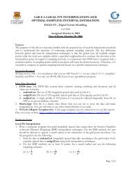
ENGO 667: Chapter 2 

Photogrammetric Triangulation 

Advanced Topics in Photogrammetry Ayman F. Habib 

1

Overview 

• Objective: Investigate the possibility of object 

space reconstruction from imagery using: 

– Single image 

– Stereo-pair 

– Single flight lines (Strip Triangulation) 

– Image blocks: 

• Block Adjustment of Independent Models (BAIM) 

• Bundle Block Adjustment 

– Special cases (resection, intersection, and stereo-pair 

orientation) 


2

Photogrammetry: The Reconstruction Process 

• The main objective of photogrammetry is to 

derive ground coordinates of object points from 

imagery. 

• We would like to investigate the feasibility of 

performing this task using single image, stereo 

image pair, or more. 

• The mathematical model we are going to use is the 

collinearity equations. 


3

Input Imagery 


4 

z 

Perspective Center 

x a 

y 

a 

ya x

Z G 

Collinearity Equations 

O G 

R( , , ) 

X O 

z i 

Y G 

c 

O i 

Y O 

Z O 


5 

pp 

+ 

y i 

a 

+ (xa, ya) X A 

x i 

Y A 

(Perspective Center) 

A 

Z A 

X G


6 

y 

Z 

Z 

r 

Y 

Y 

r 

X 

X 

r 

Z 

Z 

r 

Y 

Y 

r 

X 

X 

r 

c 

y 

y 

x 

Z 

Z 

r 

Y 

Y 

r 

X 

X 

r 

Z 

Z 

r 

Y 

Y 

r 

X 

X 

r 

c 

x 

x 

O 

A 

O 

A 

O 

A 

O 

A 

O 

A 

O 

A 

p 

a 

O 

A 

O 

A 

O 

A 

O 

A 

O 

A 

O 

A 

p 

a 

 

 

 

 

 

 

 

 

 

 

 

 

 

 

 

 

 

 

 

 

 

 

 

 

 

 

 

 

) 

( 

) 

( 

) 

( 

) 

( 

) 

( 

) 

( 

) 

( 

) 

( 

) 

( 

) 

( 

) 

( 

) 

( 

33 

23 

13 

32 

22 

12 

33 

23 

13 

31 

21 

11 

Collinearity Equations

Single Photograph 

• An image point is defined by its coordinates 

relative to the image coordinate system. 

• We have two equations (collinearity equations) in 

three unknowns (ground coordinates of the 

corresponding object point - Best Case Scenario). 

– IOP & EOP are available. 

• Consequently, this problem is under determined. 

• Conceptually: an image point will define a single 

(infinite) light ray. 

– The object point can be anywhere along this light ray. 


7

Single Photograph 

a (Image Point) 

Perspective Center 

(Single Light Ray) 


8

Stereo-Photogrammetry 

• We have the same point appearing in two images. 

– Four equations (two collinearity equations in each image) 

– Three unknowns (ground coordinates of the corresponding 

object points - Best Case Scenario) 

• IOP & EOP are available. 

• Thus, we have a redundancy of one (which will 

contribute towards the computation of the ROP). 

• Conceptually: the two image points define two light 

rays. 

– The object point is the intersection of these light rays. 


9



10

a 

PC 


Object Point (A) 


11 

PC 

a´


From Images to Object Space 

• For a stereo-pair, we can derive a 3-D 

representation of the object space covered by the 

overlap area as follows: 

– Perform RO of the stereo-pair under consideration 

(using at least five conjugate points) → stereo-model 

– Using some GCP, we can rotate, scale, and shift the 

stereo-model (AO) until it fits at the location of the 

ground control points (i.e., the residuals at the GCP are 

as small as possible). 

– For the absolute orientation, we need at least three 

ground control points (those points should not be 

collinear). 


12

Model Space 

Model Space 

From Images to Object Space (RO) 

Model Space 


13

From Images to Object Space (AO) 

Object Space 

Stereo Model 


14

Photogrammetric Triangulation 

• Objective: 

– How can we reconstruct the object space from imagery 

without the need for three ground control points in each 

stereo-model? 

• Alternatives: 

– Strip Triangulation 

– Block Adjustment of Independent Models (BAIM) 

– Bundle Block Adjustment 


15

Strip Triangulation 


16


• Strip triangulation is used for mapping linear features (such 

as road and railroad network and pipelines). 

• Given: imagery along one strip with 60% overlap between 

successive imagery 


17

• Procedure: 


– Perform RO of the first stereo-model (DRO or IRO) 

– Perform AO of the first stereo-model using 3GCP 

– Perform RO for the second model using only DRO (we 

do not want to disturb the orientation parameters for the 

second image) 

– Only scale is required to establish the AO for the 

second model. 

– Adjust the base until a point in the overlap area 

between the first and second model has the same 

elevation 

– For the remaining models, repeat the above three steps. 


18



19

• Error Propagation: 

– Similar to an open traverse, errors will increase as the 

length of the strip increases. 

• Solution: 


– Implement GCP every three or four models 

– Apply corrections polynomials 

• Correction Polynomials: 

– They are used to reduce the difference between the 

photogrammetric and geodetic coordinates of the 

control points. 


20

Correction Polynomials 

Photogrammetric Points 

Geodetic Points 


21

Z Z a p o 


• Separate polynomials are used for the X, Y, and Z 

coordinates. 

• For example: 

 

a 

g 1 

2 3 


22 

X 

 

a 

Y 

•Z g ≡ Geodetic ground coordinates 

•Z p ≡ Photogrammetric ground coordinates 

•a o ≡ Constant shift in elevation 

•a 1X ≡ Pitch along the flight line 

•a 2Y ≡ Roll across the flight line 

•a 3XY ≡ Torsion of the strip 

 

a 

XY


• Using Ground Control Points (GCP), we can solve 

for the polynomial coefficients. 

• Precaution: 

• Make sure that you have enough GCP to recover the 

polynomial coefficients 

• Use low order polynomials to avoid undulations/over 

parameterization 

• For long strips, separate them into shorter strips with 

low order polynomials and use constraints to ensure 

smooth transition between strips. 


23

Accuracy of Strip Triangulation 

• The accuracy of points measured in the strip after 

applying the correction polynomial depends on the 

number of models bridged together without 

ground control points. 

• As a rule of thumb: 

– A group of ground control points should be used every 

four models. 

• 12 models: 3 groups of ground control points 

• 16 models: 4 groups of ground control points 


24

1 

Accuracy of Strip Triangulation 

1 

sZ/ M (max) 

sXY/ M (max) 

sZ/ M (mean) 

sXY/ M (mean) 

• i number of models bridged together 

• Maximum (worst) accuracy takes place at the center 

between the control points. 


25 

i

Block Adjustment of Independent Models 

(BAIM) 


26

Block Adjustment 


27



28



29


• Given: A block of photographs with: 

– 60% overlap between successive images along the 

flight direction 

– 20% side lap between adjacent strips (across the flight 

direction) 

• Block Adjustment of Independent Models (BAIM) 

starts with model coordinate measurements after 

relative orientation. 

• Dependent or independent relative orientation can 

be used. 


30



31


• Procedure: 

– Perform RO (DRO or IRO) for all the stereo-models in 

the project 

– The models are simultaneously rotated, scaled, and 

shifted until: 

• The tie points fit together as well as possible, and 

• The residuals at the location of the ground control points are as 

small as possible. 


32

1 

6 

BAIM: Concept 


33 

2 

5 

3 

4

Tie Point 

Control Point 

1 

7 

4 

4 

Y 

Y 

I 

III 

2 

x 

x 

8 

5 

5 

5 

8 

5 

Y 

IV 

Before BAIM 

BAIM: Concept 

2 3 

Y 

II 

x 

x 

6 

6 

9 

Y G 

1 2 

I II 


34 

4 

III 

7 8 

IV 

3 

5 6 

After BAIM 

9 

X G


• BAIM can be carried out in either 2-D or 3-D. 

• Planimetric BAIM: 

– Given: 2-D model coordinates (X, Y) measured in 

relatively oriented and leveled models 

– Required: 2-D ground coordinates of these points as 

well as the transformation parameters associated with 

the involved models 

• Spatial BAIM: 

– Given: 3-D model coordinates (X, Y, Z) measured in 

relatively oriented models 

– Required: 3-D ground coordinates of these points as 

well as the transformation parameters associated with 

the involved models 


35

Planimetric BAIM 

• We start by measuring (X, Y) model coordinates 

in relatively oriented and leveled models. 

• For leveled models, the Z-axes of the model and 

ground coordinate systems are parallel. 

• For leveled models, the relationship between 

planimetric model and ground coordinates is 

represented by 2-D similarity transformation. 

• Question: how can we obtain relatively oriented 

and leveled models? 


36

Leveling Relatively Oriented Models 

• Without leveling, the mathematical relationship 

between 3-D model and ground coordinates is 

represented by 3-D similarity transformation. 

X 

 

 

Y 

 

Z 

G 

G 

G 

 

 

 

 

 

X 

 

 

Y 

 

Z 

T 

T 

T 

 

 

 

 

 

R( 

, 

, 

) 

X 

 

 

Y 

 

Z 


37 

S 

• For leveled models, ( and ) should be zeros. 

• Let’s look at the third equation: 

M 

M 

M


Z 

Z 

G 

G 

Z 

 

T 

Z 

T 

S 

S 

( r31 

X M r32 

YM 

r33 

[(sin 

 

 

sin 

(sin 

cos 

cos 

cos) 

cos 

sin 

cos 


38 

 

 

Z 

M 

Z 

] 

M 

) 

cos 

) 

sin 

X 

M 

sin ) 

Y 

• For leveling, we are only interested in recovering 

the and rotation angles. Therefore, we can set 

the rotation angle to zero. 

ZG ZT 

S ( cos 

sin X M sin YM 

cos 

cos 

ZM 

• Having four vertical control points, we can solve 

for Z T, and the scale factor. 

M 

)


• Leveling can be established in another way as 

follows: 

– Perform relative and absolute orientation for the first 

model using three ground control points. 

– Bridge other models using dependent relative 

orientation. 

• The leveling should be good enough such that the 

effect of the tilted height differences on the XYcoordinates 

is less than the photogrammetric 

accuracy of the planimetric accuracy. 


39

Effect of Leveling Errors 

• If we have leveling errors, then and are not 

exactly zero. 

– We still have residual angles (d and d). 

–Sin(d) d (in radians) cos(d) 1 

–Sin(d) d (in radians) cos(d) 1 

–dd 0.0 

X 

 

 

Y 

 

Z 

G 

G 

G 

X 

T cos 

 

 

 

 

 

 

YT 

 

S 

 

sin 

 

 

Z 

 

T d 

sin d 

cos 

sin 

cos 

d 

cos 

d 

sin 

d 

 

d 

 

 

1 

• Let’s look into the effect of leveling errors on the 

planimetric coordinates. 


40 

X 

 

 

Y 

 

Z 

M 

M 

M

X 

Y 

G 

G 

 

 

Y 


X 

T 

T 

 

 

S 

S 

[cos 

[sin 

X 


41 

X 

M 

M 

 

sin Y 

cos 

Y ] 

M 

M 

 

 

S 

S 

d 

d 

• For a constant height Z M: S dZ M and S dZ M will be 

constant and their effect can be compensated for by X T and 

Y T. 

• In other words, the mathematical relationship between 

the model and ground coordinates can still be represented 

by 2-D similarity transformation. 

• If Z M is varying, height differences will have an effect on the 

planimetric coordinates: 

• dX G = S d dZ M 

• dY G = - S d dZ M 

• This effect should be less than the planimetric accuracy. 

] 

Z 

Z 

M 

M


Planimetric Error 

t 

Leveling error 

t Height differences 

within the model 

Planimetric error should be less than the planimetric accuracy. 


42

• Given: 


– Planimetric model coordinates of tie points (X M, Y M) 

• Tie points: Points that appear in more than one model 

– Planimetric ground coordinates of control points 

• Adjustment procedure: 

– The models are displaced (X T, Y T), rotated (), and 

scaled (S) until: 

• The tie points fit together as well as possible. 

• The residuals at the ground control points are as small as 

possible. 


43

• Mathematical model: 2-D similarity transformation 

X 

 

Y 

G 

G 

 

 

 

X 

 

Y 

T 

T 

X 

G X 

T 

 

YG 

YT 

a S cos 

b S sin 


 

 

 

 

 

 

 

 

S 

cos 

 

sin 

 

a b 

 

b 

a 

sin 

cos 


44 

 

 

 

X 

Y 

M 

M 

 

 

 

 

 

 

 

 

 

X 

Y 

M 

M 

 

 

 

Non Linear Model 

Linear Model

• Unknowns: 

– Transformation parameters (XT, YT, a, and b) for each 

model 

– Ground coordinates of tie points, which appear in more 

than one model 

• Observable quantities: 


– Ground coordinates of control points 

– Model coordinates of tie points 


45

1 

6 



46 

2 

5 

3 

4

Tie Point 

Control Point 

1 

7 

4 

4 

Y 

Y 

I 

III 

Planimetric BAIM: Example 

2 

x 

x 

8 

5 

5 

5 

8 

5 

2 3 

Y 

Y 

IV 

Before BAIM 

II 

x 

x 

6 

6 

9 

Y G 

1 2 

I II 


47 

4 

III 

7 8 

IV 

3 

5 6 

After BAIM 

9 

X G

Planimetric BAIM: Example 

• Balance between observation equations and 

unknowns: 

– Unknowns: 

• 4x4=16 transformation parameters for four models 

• 5x2=10 ground coordinates of tie points 

– Observation equations: 

• 4x4x2= 32 equations derived from the 2-D similarity 

transformations 

– Redundancy: 

• 32 – 26 = 6 

• We would like to investigate the observation 

equations associated with control and tie points. 


48


49 

Planimetric BAIM: Ground Control Points 

) 

( 

) 

( 

) 

( 

) 

( 

M 

M 

G 

M 

M 

G 

Y 

M 

X 

M 

T 

Y 

G 

Y 

M 

X 

M 

T 

X 

G 

e 

Y 

a 

e 

X 

b 

Y 

e 

Y 

e 

Y 

b 

e 

X 

a 

X 

e 

X 

 

 

 

 

 

 

 

 

 

 

 

 

M 

M 

G 

M 

M 

G 

Y 

X 

Y 

M 

M 

T 

G 

Y 

X 

X 

M 

M 

T 

G 

e 

a 

e 

b 

e 

Y 

a 

X 

b 

Y 

Y 

e 

b 

e 

a 

e 

Y 

b 

X 

a 

X 

X 

 

 

 

 

 

 

 

 

 

 

 

 

M 

M 

G 

M 

M 

G 

Y 

X 

Y 

Y 

Y 

X 

X 

X 

Y 

M 

M 

T 

G 

X 

M 

M 

T 

G 

e 

a 

e 

b 

e 

v 

e 

b 

e 

a 

e 

v 

where 

v 

Y 

a 

X 

b 

Y 

Y 

v 

Y 

b 

X 

a 

X 

X 

 

 

 

 

 

 

 

 

 

 

 

 

 

 

: 

• Underlined terms: 

• Unknown quantities


50 

Planimetric BAIM: Tie Points 

) 

( 

) 

( 

) 

( 

) 

( 

M 

M 

M 

M 

Y 

M 

X 

M 

T 

G 

Y 

M 

X 

M 

T 

G 

e 

Y 

a 

e 

X 

b 

Y 

Y 

e 

Y 

b 

e 

X 

a 

X 

X 

 

 

 

 

 

 

 

 

 

 

M 

M 

M 

M 

Y 

X 

G 

M 

M 

T 

Y 

X 

G 

M 

M 

T 

e 

a 

e 

b 

Y 

Y 

a 

X 

b 

Y 

e 

b 

e 

a 

X 

Y 

b 

X 

a 

X 

 

 

 

 

 

 

 

 

 

 

 

 

0 

~ 

0 

~ 

M 

M 

M 

M 

Y 

X 

Y 

Y 

X 

X 

Y 

G 

M 

M 

T 

X 

G 

M 

M 

T 

e 

a 

e 

b 

v 

e 

b 

e 

a 

v 

where 

v 

Y 

Y 

a 

X 

b 

Y 

v 

X 

Y 

b 

X 

a 

X 

 

 

 

 

 

 

 

 

 

 

 

 

 

 

 

 

: 

0 

~ 

0 

~ 

• Underlined terms: 

• Unknown quantities


• Adding the observation equations from ground 

control and tie points, we get: 

y 

~ 

0 

1 

 

 

 

 

A 

 

A 

11 

21 

0 

A 

22 

 

 

 

x 

 

x 

1 

2 

 

 

 

 

e 

 

e 

1 

2 

 

 

 

Observation 

equations arising from GCP 

 

Observation 

equations from tie points 

• x 1 Unknown transformation parameters 

• 4 x # of models 

• x 2 Unknown ground coordinates of tie points 

• 2 x # of tie points 

• Note: (A 12) represents the partial derivatives of the 

observations arising from GCP w.r.t. the unknown ground 

coordinates of tie points (0). 


51


52 

 

 

 

 

 

 

 

 

 

 

 

 

 

 

 

 

 

 

 

 

 

 

 

 

 

 

 

 

1 

2 

1 

1 

2 

2 

1 

0 

0 

, 

0 

0 

~ 

P 

P 

e 

e 

o 

 

 

 

 

 

 

 

 

 

 

 

 

 

 

 

 

 

 

 

 

 

 

 

 

 

 

 

 

 

 

 

 

 

 

 

 

 

 

 

 

 

 

 

 

0 

~ 

0 

0 

0 

ˆ 

ˆ 

0 

0 

0 

0 

1 

2 

1 

22 

21 

11 

2 

1 

22 

21 

11 

2 

1 

22 

21 

11 

y 

P 

P 

A 

A 

A 

x 

x 

A 

A 

A 

P 

P 

A 

A 

A 

T 

T 

T 

T 

T 

T 

 

 

 

 

 

 

 

 

 

 

 

 

 

 

 

 

 

 

 

0 

~ 

ˆ 

ˆ 1 

11 

2 

1 

22 

2 

22 

21 

2 

22 

22 

2 

21 

21 

2 

21 

11 

1 

11 

Py 

A 

x 

x 

A 

P 

A 

A 

P 

A 

A 

P 

A 

A 

P 

A 

A 

P 

A 

T 

T 

T 

T 

T 

T 

 

 

 

 

 

 

 

 

 

 

 

 

 

 

 

 

 

 

 

0 

~ 

ˆ 

ˆ 1 

2 

1 

22 

12 

12 

11 

C 

x 

x 

N 

N 

N 

N 

T 

Planimetric BAIM

1 

N 

N 

11 

T 

12 

xˆ 

1 

xˆ 

1 

C 

~ 

0 


53 

 

 

N 

N 

• N11 is a block diagonal matrix with 4x4 sub-blocks 

along the diagonal. 



• We can start by solving for x2 first as follows: 

xˆ 

N C N N xˆ 

1 

11 

1 

1 

11 

T 1 

N N N N 

xˆ 

2 

22 

 

 

12 

11 

12 


12 

xˆ 

2 

 

T 1 

 

1 

T 1 

N22 

N12 

N11 

N12 

N12 

N11 

C1 

2 

 

N 

T 

12 

N 

12 

22 

1 

11 

xˆ 

2 

xˆ 

2 

C 

1 

1 

T 1 

N N N N 

where : 

np 

22 

 

12 11 12 2np 

2np 

number 

of 

tie 

points

xˆ 

xˆ 

xˆ 

xˆ 

1 

• Sequential solution of the parameters: 

• Option # 1: Solving for x2 first 

2 

1 

2 

 

 

 

N 

T 1 

N N N N 

1 

11 

22 

C 

1 

 

N 

12 

1 

11 

N 

11 

12 


54 

xˆ 

2 

12 

1 

N 

• Option # 2: Solving for x 1 first 

1 

T 

1 

N11 

N12 

N22 

N12 

C 1 

T 

N 

 

11 N12 

N22 

N12 

1 

 

 

N 

1 

22 

N 

T 

12 


xˆ 

1 

T 

12 

nm 

N 

1 

11 

where : 

C 

1 

4nm 

4nm 

 

number 

of 

models


• Sequential solution of parameters: 

– Option # 1 is useful whenever 2np < 4nm. 

– Option # 2 is useful whenever 4nm < 2np. 

–Where: 

• np number of tie points 

• nm number of models 

• Remarks: 

– Refer the coordinates within each stereo-model to its 

centroid 

• Whenever we have X M or Y M, they would reduce to zero 

(improve the sparsity of the normal equation matrix). 

– A point that appears in one model is not useful 

(eliminate it from the adjustment). 


55

X 

Y 

G 

X 

 

 

Y 

G 

G 

• Remarks: Instead of dealing with control points 

and tie points in different ways, we can do the 

following: 

– Treat all the points as tie points 

– Add pseudo observations for the ground control points 

• This approach is more general/flexible. 

G 

o 

 

o 

 

 

 

 

Y 

X 

T 

T 

 

 

Observed 

b 

a 

( X 

( X 

M 

M 

 

ground coordinates 


 

e 

X 

e 

M 

X 

) 

M 

) 

 

 

a 

X 

 

 

Y 

G 

G 

b 

( Y 


56 

 

 

 

( Y 

M 

 

M 

 

e 

 

e 

 

 

e 

X 

Y 

Y 

Go 

Go 

e 

M 

Y 

) 

 

 

 

M 

) 

e 

 

e 

 

e 

 

 

e 

X 

Y 

Go 

Go 

X 

Y 

M 

M 

 

 

 

 

 

 

~ 

~ 

0, 

0, 

G 

M

• Given: 

Spatial BAIM 

– 3-D model coordinates (XM, YM, ZM) of tie and control 

points in relatively oriented models 

– 3-D ground coordinates of control points 

• Required: 

– 3-D ground coordinates of tie points (3 np) 

• Where np is the number of tie points 

– The transformation parameters associated with each 

model (7 nm) 

• Where nm is the number of models 


57

Spatial BAIM 

• During the adjustment procedure the models are 

rotated (), scaled (S) and Shifted (X T, Y T, 

Z T) until: 

– The tie points fit together as well as possible, and 

– The residuals at the ground control points are as small 

as possible. 

• The mathematical relationship between 

corresponding model and ground coordinates is 

defined by 3-D similarity transformation. 


58

Spatial BAIM: Mathematical Model 

O G 

Z G 

R( , , ) 

S 


59 

Y G 

X T 

Z M 

O M 

Y T 

Y M 

Z T 

X G 

X M

Spatial BAIM: Mathematical Model 

X 

 

 

Y 

 

Z 

G 

G 

G 

 

 

 

 

 

X 

 

 

Y 

 

Z 

T 

T 

T 

 

 

 

 

 

R( 

, 

, 

) 

X 

 

 

Y 

 

Z 


60 

S 

M 

M 

M


61 

 

 

 

 

 

 

 

 

 

 

 

 

 

 

 

 

 

 

 

 

 

 

 

 

 

 

 

T 

G 

T 

G 

T 

G 

T 

M 

M 

M 

Z 

Z 

Y 

Y 

X 

X 

R 

S 

Z 

Y 

X 

) 

, 

, 

( 

/ 

1 

 

 

 

 

 

 

 

 

 

 

 

 

 

 

 

 

 

 

 

 

 

 

 

 

 

 

 

 

T 

G 

T 

G 

T 

G 

M 

M 

M 

Z 

Z 

Y 

Y 

X 

X 

M 

S 

Z 

Y 

X 

) 

, 

, 

( 

Spatial BAIM: Mathematical Model

1 

6 

Example (BAIM) 


62 

2 

5 

3 

4

4 

4 

1 

7 

I 

III 

Example (Spatial BAIM) 

2 

5 

5 

8 

5 

2 

8 


63 

5 

II 

IV 

3 

6 

9 

6 

Tie points 

GCP

Tie Point 

Control Point 

1 

7 

4 

4 

Y 

Y 

I 

III 

2 

x 


x 

8 

5 

5 

5 

8 

5 

2 3 

Y 

Y 

IV 

Before BAIM 

II 

x 

x 

6 

6 

9 

Y G 

1 2 

I II 


64 

4 

III 

7 8 

IV 

3 

5 6 

After BAIM 

9 

X G

• What is the balance between the observations and 

unknowns? 

– Unknowns: 

• 4 * 7 AO parameters 

• 5 * 3 GC of tie points 

• Total of 43 

– Equations: 

• 4 (models) x 4 (points/model) x 3 (equations/point) = 48 

– Redundancy: 

• 5 


• This is a non-linear system: approximations and 

partial derivatives are required. 


65

The Structure of the Observation Equations 

• Y = a(X) + e e ~ (0, 2 P -1 ) 

• Using approximate values for the unknown 

parameters (Xo ) and partial derivatives, the above 

equations can be linearized leading to the 

following equations: 

• y48x1 = A48x43 x43x1 + e48x1 e ~ (0, 2 P-1 ) 


66

The Structure of the Observation Equations 

I II III IV 2 4568 

A = y = 


67

N 

N 

Structure of the Normal Matrix 

11 

T 

12 

N 

N 

12 

22 

 

 

 

 

I II III IV 2 4 5 6 8 


68

Spatial BAIM: Final Remarks 

• To stabilize the heights along the strip, we should use the 

projection centers as tie points. 

• To stabilize the heights across the strip, we can do one of 

the following: 

– Implement a side lap of 60% 

– Use cross strips while using the projection centers as tie points 

– Apply chains of vertical control points across the strip 

– Use GPS observations at the projection centers 

• We can sequentially solve for the parameters. 

– Solve for the ground coordinates of tie points first whenever 3np < 

7nm 

– Solve for the transformation parameters for the models first 

whenever 7nm < 3np 

– Where: (np number of tie points) and (nm number of models) 


69

Accuracy of BAIM 

• Due to the reduction in the involved GCP, we 

should expect a degradation in the accuracy when 

compared with this associated with a single model. 

• Planimetric accuracy is not affected by the 

accuracy of the measured model heights or by the 

layout/distribution of vertical control points. 

• In a similar way, height accuracy is not affected 

by the accuracy of measured model planimetric 

coordinates or the the distribution of horizontal 

control points. 

• Therefore, planimetric and height accuracies can 

be treated separately. 


70

• We can derive the accuracy of the derived 

parameters after the adjustment as follows: 

D{ 

xˆ 

} 

where : 

Q{ 

xˆ 

} 

 

2 

o 

 

N 

2 

o 

1 

Q{ 

xˆ 

} 

Variance of 


observation 

unit weight 

(variance componenet) 


71 

of 

• Question: what numerical value should we expect 

for the variance component?


72 

M 

M 

M 

M 

Y 

X 

Y 

Y 

X 

X 

Y 

G 

M 

M 

T 

X 

G 

M 

M 

T 

e 

a 

e 

b 

v 

e 

b 

e 

a 

v 

where 

v 

Y 

Y 

a 

X 

b 

Y 

v 

X 

Y 

b 

X 

a 

X 

 

 

 

 

 

 

 

 

 

 

 

 

 

 

 

 

: 

0 

~ 

0 

~ 

ts 

measuremen 

coordinate 

model 

of 

Accuracy 

: 

2 

2 

2 

M 

M 

y 

x 

where 

a 

b 

b 

a 

I 

a 

b 

b 

a 

v 

v 

D 

 

 

 

 

 

 

 

 

 

 

 

 

 

 

 

 

 

 

 

 

 

 

 

 

 

BAIM: Variance Component

vx 

 

D 

 

vy 

 

a S cos 

b S sin 

a 


2 

b 

v 

D 

v 

x 

y 

2 

 

 

 

 

 

S 

S 

2 

M 

2 

2 

 

a 

 

 


73 

2 

M 

2 

I 

b 

0 

2 

2 

a 

2 

0 

b 

• If we assigned a weight of unity for the observations, then the 

estimated variance component should be o S M. 

• Variance component: variance of model coordinate 

measurements expressed in ground units 

2

Planimetric Accuracy of BAIM 

• Assume that we have: 

– Four ground control points at the corners of the block 

– The worst accuracy within the block is represented by 

max 

– The mean accuracy within the block is represented by 

mean 

• Then: 

– The accuracy deteriorates as the size of the block 

increases. 

– The worst accuracy occurs at the center of the edges of 

the block. 

• Following are some examples of expected 

accuracies. 


74


• 2 Strips x 4 Models: 


1. 

40 

2. 

25 

1. 

44 

1. 

44 


75 

o 

o 

1. 

2 

2. 

28 

2. 

28 

o 

o 

1. 

66 

o 

o 

o 

o 

1. 

40 

2. 

25 

o 

o




3. 

14 

4. 

06 

3. 

16 

3. 

16 


76 

o 

o 

2. 

17 

4. 

08 

2. 

71 

4. 

08 

o 

o 

o 

o 

o 

o 

3. 

14 

4. 

06 

o 

o


• Now, let’s investigate the effect of adding a dense 

pattern of ground control points at the boundaries 

of the block: 

– Ground control point every model across the strips of 

the block 

– Ground control point every other model along the strips 

of the block 


 

 

mean 

max 

0. 

94 

1. 

01 


77 

 

 

o 

o





1. 

01 


78 

 

 

 

 

 

 

mean 

max 

mean 

max 

mean 

max 

 

 

 

0. 

95 

1. 

00 

1. 

10 

 

 

o 

 

 

o 

1. 

03 

 

1. 

15 

o 

o 

o 

o


• By adding a dense pattern of ground control points 

along the boundaries of the block: 

– The accuracy is almost independent of the size of the 

block (i.e., it does not deteriorate as the size of the 

block increases). 

– The accuracy is almost equal to that of a single model. 

• Having a dense pattern of ground control points at 

the boundary as well as additional point at the 

center of the block do not significantly improve 

the planimetric accuracy. 


79

Empirical Formulas for Square Blocks 

• P 1: Dense chain of control points along the 

boundaries of the block: 

– Number of ground control points is proportional to the 

size of the block. 

mean ( 0. 

7 0. 

29 log10 

ns ) o 

Where : n number of strips 

s 

• P 2: 16 control points along the boundaries of the 

block (regardless of the size of the block) 

 

mean 

 

Where : n 

( 0. 

83 

0. 

02 

number 

n ) 

strips 

s 


80 

 

of 

s 

o

Empirical Formulas for Square Blocks 



 

mean 

 

Where : n 

( 0. 

83 

s 

0. 

05 

number 

n ) 

strips 



 

mean 

 

Where : n 

( 0. 

47 

s 


81 

 

 

0. 

25 

number 

of 

of 

s 

n ) 

s 

o 

o 

strips

Vertical Accuracy of BAIM 

• Height accuracy is weak across the strips. 

• Therefore, chains of vertical control points across 

the strips are recommended. 

• We use chains of vertical control points every imodels. 

• To improve the height accuracy along the upper 

and lower edges of the block, we implement a 

vertical control point every i/2 models. 


82

i 

Vertical Accuracy of BAIM 


83 

 

 

Z 

Z 

mean 

maax 

 

 

( 0. 

34 

( 0. 

27 

 

 

0. 

22 

0. 

31 

i) 

 

i) 

 

Z 

Z 

o 

o

Bundle Block Adjustment 


84


• Direct relationship between image and ground 

coordinates. 

• We measure the image coordinates in the images 

of the block. 

• Using the collinearity equations, we can relate the 

image coordinates, the corresponding ground 

coordinates, the IOP, and the EOP. 

• Using a simultaneous least squares adjustment, we 

can solve for the: 

– The ground coordinates of the tie points 

–The EOP 


85


• The image coordinate measurements and the IOP 

define a bundle of light rays. 

• The EOP define the position and the attitude of the 

bundles in space. 

• During the adjustment: The bundles are rotated 

() and shifted (Xo, Yo, Zo) until: 

– Conjugate light rays intersect as well as possible at the 

locations of object space tie points. 

– Light rays corresponding to ground control points pass 

through the object points as close as possible. 


86


Ground Control Points 

Tie Points 


87

Least Squares Adjustment in 

Photogrammetry 

• Prior to the adjustment, we need to identify: 

– The unknown parameters 

– Observable quantities 

– The mathematical relationship between the unknown 

parameters and the observable quantities 

• Linearize the mathematical relationship (if it is not 

linear) 

• Apply least squares adjustment formulas 


88

Unknown Parameters 

• Unknown parameters might include: 

– Ground coordinates of tie points (points that 

appear in more than one image) 

– Exterior orientation parameters of the involved 

imagery 

– Interior orientation parameters of the involved 

cameras (for camera calibration purposes) 


89

Observable Quantities 

• Observable quantities might include: 

– The ground coordinates of control points 

– Image coordinates of tie as well as control 

points 

– Interior orientation parameters of the involved 

cameras 

– Exterior orientation parameters of the involved 

imagery (from a GPS/INS unit onboard) 


90


91 

Mathematical Model 

) 

, 

0 

( 

~ 

) 

( 

) 

( 

) 

( 

) 

( 

) 

( 

) 

( 

) 

( 

) 

( 

) 

( 

) 

( 

) 

( 

) 

( 

1 

2 

33 

23 

13 

32 

22 

12 

33 

23 

13 

31 

21 

11 

 

 

 

 

 

 

 

 

 

 

 

 

 

 

 

 

 

 

 

 

 

 

 

 

 

 

 

 

 

 

 

 

 

 

 

 

 

P 

e 

e 

e 

y 

Z 

Z 

r 

Y 

Y 

r 

X 

X 

r 

Z 

Z 

r 

Y 

Y 

r 

X 

X 

r 

c 

y 

y 

e 

x 

Z 

Z 

r 

Y 

Y 

r 

X 

X 

r 

Z 

Z 

r 

Y 

Y 

r 

X 

X 

r 

c 

x 

x 

o 

y 

x 

y 

O 

A 

O 

A 

O 

A 

O 

A 

O 

A 

O 

A 

p 

a 

x 

O 

A 

O 

A 

O 

A 

O 

A 

O 

A 

O 

A 

p 

a

y 

y 

A 

x 

e 

 

2 

o 

 

P 

A 

1 

x 

 

n1 

n 

m 

m1 

n1 

n 

n 

Least Squares Adjustment 

e 

Gauss Markov Model 

Observation Equations 

observation 

design 

vector 

noise 

of 

variance 

matrix 

vector 

unknowns 

contaminating 

covariance 

2 

( 0, 

 

P 

the observation 

matrix 

the 

noise 


92 

e 

~ 

o 

1 

) 

of 

vector 

vector

Least Squares Adjustment 

xˆ 

D 

e~ 

ˆ 

 

 

xˆ 

2 

o 

 

( A 

 

 

y 

T 

 

 

( e~ 

PA) 

2 

o 

Axˆ 

T 

1 

( A 

Pe~ 

) 

PA) 

( n 

m) 


93 

T 

A 

/ 

T 

Py 

1

Y a( 

X ) e 

a( 

X ) is 

Y a( 

X 

Where 

X 

o 

Y a( 

X 

a 

A 

X 

o 

o 

y A x e 

Where 

: 

: 

y Y 

a( 

X 

X 

a 

) 

X 

a 

) 

X 

o 

o 

) 

Non Linear System 

the non linear function 

We use Taylor Series 

X 

is approximat e 

X 

o 

o 

Expansion 

( X X 

values 

( X X 

o 

o 

) e 

for 

) e 

unknown 

parameters 


94 

the 

(We ignore 

higher 

order 

terms) 

• Iterative solution for the unknown parameters 

• When should we stop the iterations?

Example (4 Images in Two Strips) 

1 

3 4 

5 6 

2 1 

3 4 

5 6 

I II 

3 4 

5 6 

7 

8 7 


95 

2 

3 4 

5 6 

III IV 

8 

Control Point 

Tie Point

Balance Between Observations & Unknowns 

• Number of observations: 

– 4 x 6 x 2 = 48 observations (collinearity equations) 

• Number of unknowns: 

– 4 x 6 + 3 x 4 = 36 unknowns 

• Redundancy: 

–12 

• Assumptions: 

– IOP are known and errorless. 

– Ground coordinates of control points are errorless. 


96

Structure of the Design Matrix (BA) 

• Y = a(X) + e e ~ (0, 2 P -1 ). 

• Using approximate values for the unknown 

parameters (Xo ) and partial derivatives, the above 

equations can be linearized leading to the 

following equations: 

• y48x1 = A48x36 x36x1 + e36x1 e ~ (0, 2 P-1 ). 


97

A = 

Structure of the Design Matrix (BA) 

I II III IV 3 456 

y = 


98

N 

N 

Structure of the Normal Matrix 

11 

T 

12 

N 

N 

12 

22 

 

 

 

 

I II III IV 

3 4 5 6 


99

Sample Data: 

• All the points appear in all the images. 

• Two images were captured by each camera. 

• 2 cameras 

• 4 images 

• 16 points 


100

Structure of the Normal Matrix: Example 


101

Observation Equations 

y 

2 

n1 

nm 

m1 

n1 

o 

A x e e ~ ( 0, 

P 

y 

y 

n1 

n1 

 

 

A 

1 

n6 

m1 

1 

1 

A1 

A2 

en1 

n6 

m1 

x 

6m1 

1 

n3 

m2 


102 

 

A 

2 

n3 

m2 

x 

x 

 

2 

6m1 

1 

x 

3m21 

2 

 

 

3m21 

• n Number of observations (image coordinate measurements) 

• m Number of unknowns: 

• m 1 Number of images 6 m 1 (EOP of the images) 

• m 2 Number of tie points 3 m 2 (ground coordinates of tie points) 

• m = 6 m 1 + 3 m 2 

 

e 

n1 

1 

)


103 

Normal Equation Matrix 

 

 

 

 

 

 

 

 

 

 

 

 

 

 

 

 

 

 

 

 

 

 

 

 

 

 

 

 

 

 

 

 

 

 

 

 

 

 

 

 

 

 

 

 

 

 

 

 

 

 

 

1 

2 

3 

1 

1 

6 

2 

1 

2 

3 

2 

3 

1 

6 

2 

3 

2 

3 

1 

6 

1 

6 

1 

6 

2 

1 

2 

1 

2 

1 

2 

1 

2 

1 

1 

) 

3 

6 

( 

22 

12 

12 

11 

2 

1 

2 

1 

) 

3 

6 

( 

) 

3 

6 

( 

m 

m 

m 

m 

m 

m 

m 

m 

m 

m 

C 

C 

Py 

A 

Py 

A 

y 

P 

A 

A 

C 

N 

N 

N 

N 

N 

A 

A 

P 

A 

A 

N 

T 

T 

T 

T 

m 

m 

T 

T 

T 

m 

m 

m 

m





N 

 

N 

 

11 

T 

12 


6m1 

6 

m1 

3m26 

m1 

N 

N 

12 

22 

6m1 

3m2 

3m23 

m2 

xˆ 

 

xˆ 

 

C 

 

C 

 


104 

 

 

 

1 

2 

6m1 

1 

3m21 

 

 

 

 

1 

2 

6 m11 

3m21

N 

xˆ 

xˆ 

2 

1 

Reduction of the Normal Equation Matrix 

T 

12 

3m26 

m1 

3m21 

6m1 

1 

 

 

N 

N 

11 

T 

12 

6m1 

6 

m1 

3m26 

m1 

xˆ 

1 

xˆ 

• Solving for x 2 first: 

6m1 

1 

1 

6 m11 

 

 

N 

6m1 

3m2 

3m23 

m2 

3m21 

3m21 

6 m11 

3m21 


105 

N 

12 

22 

 

1 

1 

N C N N xˆ 

6 m16 

m1 

N22 T 

N12 

1 

N11 

N12 

1C2 T 

N12 

1 

N11 

C1 

 

1 

N C 

1 

N N xˆ 

 

11 

11 

3m23 

m2 

6 m16 

m1 

1 

1 

6m1 

1 

6m1 

1 

3m26 

m1 

11 

11 

6m1 

6 

m1 

6m1 

6 

m1 

6m1 

6 

m1 

12 

12 

6m1 

3m2 

6m1 

3m2 

6m1 

3m2 

2 

2 

3m21 

3m21 

xˆ 

2 

xˆ 

 

2 

N 

3m21 

22 

 

 

3m23 

m2 

C 

xˆ 

1 

C 

2 

2 

3m21 

3m26 

m1 

 

C 

2 

3m21 

6m1 

6 

m1 

•3m 2 < 6m 1 

• Remember: N 11 is a block diagonal matrix with 6x6 sub-blocks 


6 m11

N 

xˆ 

1 

xˆ 

6 m16 

m1 

6m1 

1 

2 


11 

3m21 

 

 

xˆ 

1 

N 

N 

6 m11 

11 

T 

12 

6m1 

6 

m1 

3m26 

m1 

xˆ 

1 

xˆ 

• Solving for x 1 first: 

6m1 

1 

1 

6 m11 

 

 

N 

6m1 

3m2 

3m23 

m2 

3m21 

3m21 

6 m11 

3m21 


106 

N 

12 

22 

xˆ 

2 

xˆ 

2 

 

 

C 

1 

C 

 

1 

1 

T 

N C N N xˆ 

N11 N12 

1 

N22 

T 

N12 

1C1N12 1 

N22 

C2 

 

1 

N C 

1 

N 

T 

N xˆ 

 

6m1 

6m1 

22 

 

3m23 

m2 

N 

12 

3m23 

m2 

2 

3m21 

6m1 

3m2 

22 

3m23 

m2 

22 

3m23 

m2 

3m23 

m2 

2 

3m21 

12 

3m26 

m1 

3m26 

m1 

22 

1 

3m23 

m2 

6m1 

1 

6m1 

1 

12 

3m26 

m1 

1 

6m1 

3m2 

2 

6m1 

1 

 

C 

1 

6m1 

1 

3m22 

m2 

•6m 1 < 3m 2 

• Remember: N 22 is a block diagonal matrix with 3x3 sub-blocks 


3m21


• Variance covariance matrix of the estimated parameters: 

D{ xˆ 

} 

D{ 

xˆ 

1 

2 

6 m11 

3 m21 

} 

1 

1 

T 

N N N N 

2 

o 116 

m16 

m1 

126 

m 3m 

223m 

3m 

123m 

6 

m 


107 

1 

2 

1 

T 

1 

 

N N N N 

2 

o 223m 

3m 

123m 

6 

m 116 

m 6 

m 126 

m 3m 

2 

2 

2 

1 

2 

1 

2 

1 

2 

1 

1 

2

Building the Normal Equation Matrix 

• We would like to investigate the possibility of 

sequentially building up the normal equation 

matrix without fully building the design matrix. 

• (xij, yij) image coordinates of the ith point in the jth image 

y A x A x e 

y 

21 

21 

ij 

ij 

 

1 

26ij 

1 A1 

A2 

e21ij 

26ij 

1 

61 

j 

23ij 

23ij 

x 

 


108 

2 

x 

61 

j 

2 

31i 

2 

 

31i 

21 

ij


109 

 

 

 

 

 

 

 

 

 

 

 

 

 

 

 

 

 

 

 

 

 

 

 

 

 

 

 

 

 

 

 

 

 

 

 

 

 

 

 

 

 

 

 

 

 

 

 

 

 

 

 

 

 

 

 

 

 

 

 

 

 

 

 

 

 

 

 

 

 

 

 

 

 

 

 

 

 

 

 

 

 

 

 

 

 

 

 

 

 

 

 

ij 

ij 

ij 

ij 

i 

j 

ij 

ij 

ij 

ij 

ij 

ij 

ij 

ij 

ij 

ij 

ij 

i 

j 

ij 

ij 

ij 

ij 

ij 

i 

j 

ij 

ij 

ij 

y 

P 

A 

y 

P 

A 

x 

x 

A 

P 

A 

A 

P 

A 

A 

P 

A 

A 

P 

A 

y 

P 

A 

A 

x 

x 

A 

A 

P 

A 

A 

e 

x 

x 

A 

A 

y 

ij 

T 

ij 

T 

ij 

T 

ij 

T 

ij 

T 

ij 

T 

ij 

T 

T 

ij 

T 

T 

1 

2 

2 

1 

2 

1 

2 

1 

2 

2 

1 

2 

2 

1 

1 

1 

1 

2 

2 

1 

2 

1 

2 

1 

2 

1 

1 

2 

2 

1 

2 

1 

1 

2 

2 

3 

2 

6 

1 

3 

1 

6 

3 

2 

2 

3 

6 

2 

2 

3 

3 

2 

2 

6 

6 

2 

2 

6 

2 

3 

2 

6 

1 

3 

1 

6 

3 

2 

6 

2 

2 

3 

2 

6 

1 

3 

1 

6 

3 

2 

6 

2 

Normal Equation Matrix

A 

 

A 

 

N 

 

 

N 

T 

1 

62ij 

T 

2 

32ij 

11 

T 

12 

ij 

ij 

P 

ij 

P 

ij 

A 

1 

A 

N 

N 

1 

26ij 

26ij 

12 

22 

ij 

ij 


 

 

 

99 

A 

A 

T 

1 

62ij 

T 

2 

32ij 

x 

 

x 

 

1 

61 

j 

2 

P 

ij 

P 

31i 

ij 

A 

A 

 

 

 

91 

91 


110 

2 

2 

23ij 

23ij 

x 

 

x 

 

C 

 

 

C 

1 

1 

2 

61 

j 

2 

ij 

31i 

ij 

 

 

 

 

 

 

 

A 

 

A 

 

T 

1 

62ij 

T 

2 

32ij 

• Note: We cannot solve this matrix for the: 

• The Exterior Orientation Parameters of the j th image 

• The ground coordinates of the i th point 

P 

ij 

P 

ij 

y 

y 

21 

ij 

21 

ij

N 

 

N 

 

11 

T 

12 


6m1 

6 

m1 

3m26 

m1 

N 

N 

12 

22 

6m1 

3m2 

3m23 

m2 

xˆ 

 

xˆ 

 

C 

 

C 

 


111 

 

 

 

1 

2 

6m1 

1 

3m21 

 

 

 

 

1 

2 

6 m11 

3m21 

• Question: How can we sequentially build the above matrices? 

• Assumption: All the points are common to all the images.

N 

11 

( 6m1 

6 

m1 

) 

 

 

i 

 

 

 

 

 

 

 

 

 

 

 

m 

2 

 

1 

N 

0 

0 

 

 

0 

11 

i1 

N 11 -Matrix 

m 

2 

 

i 1 

0 

N 

0 

 

 

0 


112 

11 

i 2 

• If all the points are not common to all the images: 

• The summation should be carried over all the points 

that appear in the image under consideration. 

m 

2 

 

i 1 

0 

0 

N 

 

 

0 

11 

i 3 

 

 

 

 

 

 

 

 

 

 

 

 

m 

2 

 

i 1 

0 

0 

0 

 

 

N 

11 

im1

N 

22 

( 3m23 

m2 

) 

 

 

 

 

 

 

 

 

 

 

 

 

 

 

m 

1 

 

j 1 

N 

0 

0 

 

 

0 

22 

1 j 

N 22 -Matrix 

m 

1 

 

j 1 

0 

N 

0 

 

 

0 


113 

22 

2 j 

• If all the points are not common to all the images: 

• The summation should be carried over all the images 

within which the point under consideration appears. 

m 

1 

 

j 1 

0 

0 

N 

 

 

0 

22 

3 j 

 

 

 

 

 

 

 

 

 

 

 

 

m 

1 

 

j 1 

0 

0 

0 

 

 

N 

22 

m2 

j

N 

12 

( 6 m13 

m2 

) 

N12 

 

 

N12 

N12 

 

 

 

 

N 

121 

N 12 -Matrix 

11 

12 

13 

m1 

N 

N 

N 

N 


114 

12 

12 

12 

 

 

12 

21 

22 

23 

2 m1 

N 

N 

N 

N 

12 

12 

12 

 

 

12 

31 

32 

23 

3m1 

 

 

 

 

• If point “i” does not appear in image “j”: 

•(N 12) ij = 0 

 

 

 

 

 

 

 

 

N 

N 

N 

N 

12 

12 

12 

 

 

12 

m21 

m2 

2 

m2 

3 

m2m1

C 

1 

6m1 

1 

 

 

i 

 

 

i 

 

 

i 

 

 

 

 

 

 

i 

m 

2 

 

1 

m 

2 

 

1 

m 

2 

 

1 

m 

2 

 

1 

C 

C 

C 

 

 

C 

1 

1 

1 

1 

i1 

i 2 

i 3 

im1 

 

 

 

 

 

 

 

 

 

 

 

 

 

 

C - Matrix 

3m21 

 

 

 

 

 

 

 

 

 

 

 

 

 

 

• Once again, we assumed that all the points are common to all 

the images. 


115 

C 

2 

m 

1 

 

j 1 

m 

1 

 

j 1 

m 

1 

 

j 1 

m 

1 

 

j 1 

C 

C 

C 

 

 

C 

2 

2 

2 

2 

1 j 

2 j 

3 j 

m2 

j

Accuracy of Bundle Block Adjustment 

• The accuracy of the estimated EOP as well as the 

ground coordinates of tie points can be obtained 

by the product of: 

– The estimated variance component, and 

– The inverse of the normal equation matrix (cofactor 

matrix) 

• For planning purposes, we can use the same rules 

applied for BAIM. 

• However, the accuracy of a single model has to be 

modified. 


116

Accuracy of Bundle Block Adjustment 

• Accuracy of a single model: If we have 

– Bundle block adjustment with additional parameters 

that compensate for various distortions 

– Regular blocks with 60%overlap and 20% side lap 

– Signalized targets 

XY 3 

m 

Z 0. 

003% 

of the camera principal distance 

Z 0. 

004% 

of the camera principal distance 

These accuracies are given in the image space 

(NA and WA cameras) 

(SWA cameras) 


117

Camera Classification 

• < 75 Normal angle camera (NA) 

• 100 > > 75 Wide angle camera (WA) 

• > 100 Super wide angle camera (SWA) 


118

Advantages of Bundle Block Adjustment 

• Most accurate triangulation technique since we have direct 

transformation between image and ground coordinates 

• Straight forward to include parameters that compensate for 

various deviations from the collinearity model 

• Straight forward to include additional observations: 

– GPS observations at the exposure stations 

– Object space distances 

• Can be used for normal, convergent, aerial, and close range 

imagery 

• After the adjustment, the EOP can be set on analogue and 

analytical plotters for compilation purposes. 


119

Disadvantages of Bundle Block Adjustment 

• Model is non linear: approximations as well as 

partial derivatives are needed. 

• Requires computer intensive computations 

• Analogue instruments cannot be used (they cannot 

measure image coordinate measurements). 

• The adjustment cannot be separated into 

planimetric and vertical adjustment. 


120

Strip Triangulation: Final Remarks 

• Elementary Unit: Stereo models after absolute 

orientation 

• Measurements: Photogrammetric ground 

coordinates 

• Mathematical model: Polynomial corrections 

• Instruments: Analogue and analytical plotters as 

well as Digital Photogrammetric Workstations 

(DPW) 

• Required computer power: Low 

• Expected accuracy: Low 


121

BAIM: Final Remarks 

• Elementary Unit: Stereo models after relative 

orientation 

• Measurements: Model coordinates 

• Mathematical model: 2-D/3-D similarity 

transformation 

• Instruments: Analogue and analytical plotters as 

well as Digital Photogrammetric Workstations 

(DPW) 

• Required computer power: Large 

• Expected accuracy: Medium 


122

Bundle Adjustment: Final Remarks 

• Elementary Unit: Images 

• Measurements: Image coordinates 

• Mathematical model: Collinearity equations 

• Instruments: Comparators, analytical plotters, and 

Digital Photogrammetric Workstations (DPW) 

• Required computer power: Very large 

• Expected accuracy: High 


123

• Resection 

• Intersection 

• Stereo-pair orientation 

• Relative orientation 

– Discussed in chapter 1 

Special Cases 


124

Resection 

• We are dealing with one image. 

• We would like to determine the EOP of this image 

using GCP. 

• Q: What is the minimum GCP requirements? 

– At least 3 non-collinear GCP are required to estimate 

the 6 EOP. 

– At least 5 non-collinear (well distributed in 3-D) GCP 

are required to estimate the 6 EOP and the 3 IOP (x p, 

y p, c). 

• Critical surface: 

– The GCP and the perspective center lie on a common 

cylinder 


125

Resection 

exterior orientation 

interior orientation 


126

Resection - Critical Surface 


127

Intersection 

• We are dealing with two images. 

• The EOP of these images are available. 

• The IOP of the involved camera(s) are also 

available. 

• We want to estimate the ground coordinates of 

points in the overlap area. 

• For each tie point, we have: 

– 4 Observation equations 

– 3 Unknowns 

– Redundancy = 1 

• Non-linear model: approximations are needed. 


128

a 

PC 

Intersection 

Object Point (A) 


129 

PC 

a´

O l 

Intersection: Linear Model 

V l 


130 

B 

X 

 

 

 

Y 

 

 

Z 

V r 

O r

V 

 

V 

r 

l 

 

 

 

B 

 

R 

R 


X 

 

Y 

 

 

Z 

l 

r 

O 

O 

O 

l 

r 

r 

r 

r 

( , , 

( , , 

l 

X Ol 

 

YOl 

 

Z 

Ol 

 

xl 

xp 

 

 

) 

yl 

y p 

 

c 

xr 

xp 

 

 

) 

yr 

y p 

 

c 

r 

• These vectors are given w.r.t.the 

ground coordinate system. 


131

V 

l 

 

X 

 

Y 

 

 

Z 

o 

o 

o 

r 

r 

r 

 

B 

 

 

 

 

X 

Yo 

Z 

 

V 

l 

o 

o 

l 

l 

r 


 

 

 

 

 

 

R 

x 

 

 

y 

 

x 

y 

c 

x 

 

 

y 

 


132 

l 

p 

 

 

 

 

 

R 

( , , ) l p 

( , , ) 

l 

l 

l 

• Three equations in two unknowns () 

• They are linear equations. 

r 

r 

r 

r 

r 

x 

y 

c 

p 

p


133 

 

 

 

 

 

 

 

 

 

 

 

 

 

 

 

 

 

 

 

 

 

 

 

 

 

 

 

 

 

 

 

 

 

 

 

c 

y 

y 

x 

x 

R 

Z 

Y 

X 

Z 

Y 

X 

p 

l 

p 

l 

O 

O 

O 

l 

l 

l 

l 

l 

l 

) 

, 

, 

( 

 

 

 

 

 

 

 

 

 

 

 

 

 

 

 

 

 

 

 

 

 

 

 

 

 

 

 

 

 

 

 

 

 

 

 

 

 

 

c 

y 

y 

x 

x 

R 

Z 

Y 

X 

Z 

Y 

X 

p 

r 

p 

r 

O 

O 

O 

r 

r 

r 

r 

r 

r 

) 

, 

, 

( 

 

 

 

Or: 

Intersection: Linear Model

• Given: 

Stereo-pair Orientation 

– Stereo-pair: two images with at least 50% overlap 

– Image coordinates of some tie points 

– Image and ground coordinates of control points 

• Required: 

– The ground coordinates of the tie points 

– The EOP of the involved images 

• Mini-Bundle Adjustment Procedure 


134

• Example: 

–Given: 

• 1 Stereo-pair 

• 20 tie points 

• No ground control points 

– Question: 

• Can we estimate the ground coordinates of the tie points as 

well as the exterior orientation parameters of that stereo-pair? 

–Answer: 

• NO 

Stereo-pair Orientation 


135

x - Digital Photogrammetry Research Group

Create successful ePaper yourself

Delete template?

Save as template?