9.3 THE SIMPLEX METHOD: MAXIMIZATION
9.3 THE SIMPLEX METHOD: MAXIMIZATION
9.3 THE SIMPLEX METHOD: MAXIMIZATION

You also want an ePaper? Increase the reach of your titles
YUMPU automatically turns print PDFs into web optimized ePapers that Google loves.
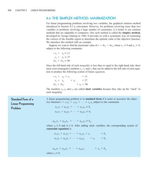
494 CHAPTER 9 LINEAR PROGRAMMING<br />
Standard Form of a<br />
Linear Programming<br />
Problem<br />
<strong>9.3</strong> <strong>THE</strong> <strong>SIMPLEX</strong> <strong>METHOD</strong>: <strong>MAXIMIZATION</strong><br />
For linear programming problems involving two variables, the graphical solution method<br />
introduced in Section 9.2 is convenient. However, for problems involving more than two<br />
variables or problems involving a large number of constraints, it is better to use solution<br />
methods that are adaptable to computers. One such method is called the simplex method,<br />
developed by George Dantzig in 1946. It provides us with a systematic way of examining<br />
the vertices of the feasible region to determine the optimal value of the objective function.<br />
We introduce this method with an example.<br />
Suppose we want to find the maximum value of z 4x1 6x2 , where x1 0 and x2 0,<br />
subject to the following constraints.<br />
x 1 5x 2 11<br />
x1 5x2 27<br />
2x1 5x2 90<br />
Since the left-hand side of each inequality is less than or equal to the right-hand side, there<br />
must exist nonnegative numbers s1 , s2 and s3 that can be added to the left side of each equation<br />
to produce the following system of linear equations.<br />
x 1 5x 2 s 1 s 2 s 3 11<br />
x 1 5x 2 s 1 s 2 s 3 27<br />
2x 1 5x 2 s 1 s 2 s 3 90<br />
The numbers s1 , s2 and s3 are called slack variables because they take up the “slack” in<br />
each inequality.<br />
A linear programming problem is in standard form if it seeks to maximize the objective<br />
function z c1x1 c2x2 subject to the constraints<br />
. . . cnxn .<br />
am1x1 am2x2 . . . a21x1 a22x2 <br />
amnxn bm . . . a2nxn b2 where xi 0 and bi 0. After adding slack variables, the corresponding system of<br />
constraint equations is<br />
where s i 0.<br />
a 11 x 1 a 12 x 2 . . . a 1n x n b 1<br />
a 11 x 1 a 12 x 2 . . . a 1n x n s 1 b 1<br />
a 21 x 1 a 22 x 2 . . . a2n x n s 2<br />
b2 .<br />
a m1 x 1 a m2 x 2 . . . a mn x n s m b m
REMARK: Note that for a linear programming problem in standard form, the objective<br />
function is to be maximized, not minimized. (Minimization problems will be discussed in<br />
Sections 9.4 and 9.5.)<br />
A basic solution of a linear programming problem in standard form is a solution<br />
x1 , x2 , . . . , xn , s1 , s2 , . . . , sm of the constraint equations in which at most m variables are<br />
nonzero––the variables that are nonzero are called basic variables. A basic solution for<br />
which all variables are nonnegative is called a basic feasible solution.<br />
The Simplex Tableau<br />
The simplex method is carried out by performing elementary row operations on a matrix<br />
that we call the simplex tableau. This tableau consists of the augmented matrix corresponding<br />
to the constraint equations together with the coefficients of the objective function<br />
written in the form<br />
In the tableau, it is customary to omit the coefficient of z. For instance, the simplex tableau<br />
for the linear programming problem<br />
z 4x 1 6x 2<br />
is as follows.<br />
x1 x2 s1 s2 s3 b<br />
Basic<br />
Variables<br />
1 1 1 0 0 11 s1 1 1 0 1 0 27 s2 2 5 0 0 1 90 s3 4<br />
6<br />
SECTION <strong>9.3</strong> <strong>THE</strong> <strong>SIMPLEX</strong> <strong>METHOD</strong>: <strong>MAXIMIZATION</strong> 495<br />
c 1 x 1 c 2 x 2 . . . c n x n 0s 1 0s 2 . . . 0 s m z 0.<br />
0 0 0 0<br />
↑<br />
Current z–value<br />
Objective function<br />
x1 5x2 s1 s2 s3 11<br />
} x1 5x2 s1 s2 s3 27<br />
Constraints<br />
2x1 5x2 s1 s2 s3 90<br />
For this initial simplex tableau, the basic variables are s1 , s2 , and s3 , and the nonbasic<br />
variables (which have a value of zero) are x1 and x2. Hence, from the two columns that are<br />
farthest to the right, we see that the current solution is<br />
x1 0, x2 0, s1 11, s2 27, and s3 90.<br />
This solution is a basic feasible solution and is often written as<br />
x1 , x2 , s1 , s2 , s3 0, 0, 11, 27, 90.
496 CHAPTER 9 LINEAR PROGRAMMING<br />
The entry in the lower–right corner of the simplex tableau is the current value of z. Note<br />
that the bottom–row entries under x1 and x2 are the negatives of the coefficients of x1 and<br />
x2 in the objective function<br />
To perform an optimality check for a solution represented by a simplex tableau, we look<br />
at the entries in the bottom row of the tableau. If any of these entries are negative (as<br />
above), then the current solution is not optimal.<br />
Pivoting<br />
z 4x 1 6x 2 .<br />
Once we have set up the initial simplex tableau for a linear programming problem, the simplex<br />
method consists of checking for optimality and then, if the current solution is not optimal,<br />
improving the current solution. (An improved solution is one that has a larger z-value<br />
than the current solution.) To improve the current solution, we bring a new basic variable<br />
into the solution––we call this variable the entering variable. This implies that one of the<br />
current basic variables must leave, otherwise we would have too many variables for a basic<br />
solution––we call this variable the departing variable. We choose the entering and<br />
departing variables as follows.<br />
1. The entering variable corresponds to the smallest (the most negative) entry in the<br />
bottom row of the tableau.<br />
2. The departing variable corresponds to the smallest nonnegative ratio of biaij, in the<br />
column determined by the entering variable.<br />
3. The entry in the simplex tableau in the entering variable’s column and the departing<br />
variable’s row is called the pivot.<br />
Finally, to form the improved solution, we apply Gauss-Jordan elimination to the column<br />
that contains the pivot, as illustrated in the following example. (This process is called<br />
pivoting.)<br />
EXAMPLE 1 Pivoting to Find an Improved Solution<br />
Use the simplex method to find an improved solution for the linear programming problem<br />
represented by the following tableau.<br />
Basic<br />
x1 x2 s1 s2 s3 b Variables<br />
1 1 1 0 0 11 s1 1 1 0 1 0 27 s2 2 5 0 0 1 90 s3 4<br />
6<br />
0 0 0 0<br />
The objective function for this problem is z 4x 1 6x 2 .
Solution Note that the current solution x1 0, x2 0, s1 11, s2 27, s3 90 corresponds to<br />
a z–value of 0. To improve this solution, we determine that x2 because 6 is the smallest entry in the bottom row.<br />
is the entering variable,<br />
x1 x2 s1 s2 s3 b<br />
Basic<br />
Variables<br />
1 1 1 0 0 11 s1 1 1 0 1 0 27 s2 2 5 0 0 1 90 s3 4 6<br />
↑<br />
Entering<br />
0 0 0 0<br />
To see why we choose x2 as the entering variable, remember that z 4x1 6x2 . Hence, it<br />
appears that a unit change in x2 produces a change of 6 in z, whereas a unit change in x1 produces a change of only 4 in z.<br />
To find the departing variable, we locate the bi’s that have corresponding positive elements<br />
in the entering variables column and form the following ratios.<br />
11<br />
1<br />
Here the smallest positive ratio is 11, so we choose s1 as the departing variable.<br />
Basic<br />
x1 x2 s1 s2 s3 b Variables<br />
1 1 1 0 0 11 s1 ← Departing<br />
1 1 0 1 0 27 s2 2 5 0 0 1 90 s3 4 6<br />
↑<br />
Entering<br />
0 0 0 0<br />
Note that the pivot is the entry in the first row and second column. Now, we use Gauss-<br />
Jordan elimination to obtain the following improved solution.<br />
1<br />
1<br />
2<br />
4<br />
11, 27<br />
1<br />
1<br />
1<br />
5<br />
6<br />
Before Pivoting After Pivoting<br />
1<br />
0<br />
0<br />
0<br />
27, 90<br />
5<br />
0<br />
1<br />
0<br />
0<br />
0<br />
0<br />
1<br />
0<br />
18<br />
11<br />
27<br />
90<br />
0<br />
The new tableau now appears as follows.<br />
SECTION <strong>9.3</strong> <strong>THE</strong> <strong>SIMPLEX</strong> <strong>METHOD</strong>: <strong>MAXIMIZATION</strong> 497<br />
1<br />
<br />
2<br />
7<br />
10<br />
1<br />
0<br />
0<br />
0<br />
1<br />
1<br />
5<br />
6<br />
0<br />
1<br />
0<br />
0<br />
0<br />
0<br />
1<br />
0<br />
11<br />
16<br />
35<br />
66
498 CHAPTER 9 LINEAR PROGRAMMING<br />
x1 x2 s1 s2 s3 b<br />
Basic<br />
Variables<br />
1 1 1 0 0 11 x2 2 0 1 1 0 16 s2 7 0 5 0 1 35 s3 10<br />
0 6 0 0 66<br />
Note that x2 has replaced s1 in the basis column and the improved solution<br />
x 1 , x 2 , s 1 , s 2 , s 3 0, 11, 0, 16, 35<br />
has a z-value of<br />
z 4x 1 6x 2 40 611 66.<br />
In Example 1 the improved solution is not yet optimal since the bottom row still has a<br />
negative entry. Thus, we can apply another iteration of the simplex method to further improve<br />
our solution as follows. We choose x1 as the entering variable. Moreover, the smallest<br />
nonnegative ratio of 111, 162 8, and 357 5 is 5, so s3 is the departing<br />
variable. Gauss-Jordan elimination produces the following.<br />
1<br />
<br />
2<br />
7<br />
10<br />
1<br />
0<br />
0<br />
0<br />
1<br />
1<br />
5<br />
6<br />
Thus, the new simplex tableau is as follows.<br />
Basic<br />
x 1 x 2 s 1 s 2 s 3 b Variables<br />
2<br />
0 1 0 16 x2 0 0 1 6 s2 1 0 0<br />
1<br />
5 x1 5<br />
2<br />
7<br />
7<br />
3<br />
7<br />
7<br />
7<br />
10<br />
7<br />
0 0 0 116<br />
8<br />
7<br />
0<br />
1<br />
0<br />
0<br />
1<br />
7<br />
0<br />
0<br />
1<br />
0<br />
11<br />
16<br />
35<br />
66<br />
1<br />
<br />
2<br />
1<br />
10<br />
In this tableau, there is still a negative entry in the bottom row. Thus, we choose s1 as the<br />
entering variable and s2 as the departing variable, as shown in the following tableau.<br />
0<br />
0<br />
1<br />
0<br />
1<br />
0<br />
0<br />
0<br />
1<br />
0<br />
0<br />
0<br />
2<br />
7<br />
3<br />
7<br />
5<br />
7<br />
8<br />
7<br />
1<br />
1<br />
5<br />
7<br />
6<br />
0<br />
1<br />
0<br />
0<br />
0<br />
1<br />
0<br />
0<br />
1<br />
7<br />
2<br />
7<br />
1<br />
7<br />
10<br />
7<br />
0<br />
0<br />
1<br />
7<br />
0<br />
16<br />
6<br />
5<br />
116<br />
11<br />
16<br />
5<br />
66
Figure 9.18<br />
x2 25<br />
20<br />
15<br />
10<br />
5<br />
(0, 11)<br />
(0, 0)<br />
(5, 16)<br />
5<br />
(15, 12)<br />
(27, 0)<br />
x1 10 15 20 25 30<br />
x1 x2 s1 s2 s3 b<br />
Basic<br />
Variables<br />
0 1 0 16 x2 0 0 1 6 s2 ← Departing<br />
1 0 0 5 x1 0 0 <br />
↑<br />
Entering<br />
0<br />
10<br />
7 116<br />
8<br />
<br />
1<br />
7<br />
7<br />
5<br />
<br />
7<br />
2<br />
2<br />
7<br />
1<br />
7<br />
3<br />
7<br />
7<br />
By performing one more iteration of the simplex method, we obtain the following tableau.<br />
(Try checking this.)<br />
Basic<br />
x1 x2 s1 s2 s3 b Variables<br />
0 1 0 12 x2 0 0 1 14 s1 1 0 0 15 x1 1<br />
<br />
5<br />
2<br />
3 3<br />
7<br />
3 3<br />
0 0 0 132 ← Maximum z-value<br />
In this tableau, there are no negative elements in the bottom row. We have therefore determined<br />
the optimal solution to be<br />
with<br />
x 1 , x 2 , s 1 , s 2 , s 3 15, 12, 14, 0, 0<br />
z 4x 1 6x 2 415 612 132.<br />
REMARK: Ties may occur in choosing entering and/or departing variables. Should this<br />
happen, any choice among the tied variables may be made.<br />
Because the linear programming problem in Example 1 involved only two decision variables,<br />
we could have used a graphical solution technique, as we did in Example 2, Section<br />
9.2. Notice in Figure 9.18 that each iteration in the simplex method corresponds to moving<br />
from a given vertex to an adjacent vertex with an improved z-value.<br />
0, 0<br />
z 0<br />
The Simplex Method<br />
2<br />
3<br />
8<br />
3<br />
0, 11<br />
z 66<br />
SECTION <strong>9.3</strong> <strong>THE</strong> <strong>SIMPLEX</strong> <strong>METHOD</strong>: <strong>MAXIMIZATION</strong> 499<br />
1<br />
3<br />
2<br />
3<br />
5, 16<br />
z 116<br />
15, 12<br />
z 132<br />
We summarize the steps involved in the simplex method as follows.
500 CHAPTER 9 LINEAR PROGRAMMING<br />
The Simplex Method<br />
(Standard Form)<br />
To solve a linear programming problem in standard form, use the following steps.<br />
1. Convert each inequality in the set of constraints to an equation by adding slack<br />
variables.<br />
2. Create the initial simplex tableau.<br />
3. Locate the most negative entry in the bottom row. The column for this entry is called<br />
the entering column. (If ties occur, any of the tied entries can be used to determine<br />
the entering column.)<br />
4. Form the ratios of the entries in the “b-column” with their corresponding positive<br />
entries in the entering column. The departing row corresponds to the smallest non-<br />
negative ratio biaij .<br />
(If all entries in the entering column are 0 or negative, then there<br />
is no maximum solution. For ties, choose either entry.) The entry in the departing row<br />
and the entering column is called the pivot.<br />
5. Use elementary row operations so that the pivot is 1, and all other entries in the<br />
entering column are 0. This process is called pivoting.<br />
6. If all entries in the bottom row are zero or positive, this is the final tableau. If not, go<br />
back to Step 3.<br />
7. If you obtain a final tableau, then the linear programming problem has a maximum<br />
solution, which is given by the entry in the lower-right corner of the tableau.<br />
Note that the basic feasible solution of an initial simplex tableau is<br />
x 1 , x 2 , . . . , x n , s 1 , s 2 , . . . , s m 0, 0, . . . , 0, b 1 , b 2 , . . . , b m .<br />
This solution is basic because at most m variables are nonzero (namely the slack variables).<br />
It is feasible because each variable is nonnegative.<br />
In the next two examples, we illustrate the use of the simplex method to solve a<br />
problem involving three decision variables.<br />
EXAMPLE 2 The Simplex Method with Three Decision Variables<br />
Use the simplex method to find the maximum value of<br />
z 2x1 x2 2x3 Objective function<br />
subject to the constraints<br />
2x 1 2x 2 2x 3 10<br />
2x 1 2x 2 2x 3 20<br />
2x 1 2x 2 2x 3 25<br />
where x1 0, x2 0, and x3 0.<br />
Solution Using the basic feasible solution<br />
x 1 , x 2 , x 3 , s 1 , s 2 , s 3 0, 0, 0, 10, 20, 5<br />
the initial simplex tableau for this problem is as follows. (Try checking these computations,<br />
and note the “tie” that occurs when choosing the first entering variable.)
Basic<br />
x 1 x 2 x 3 s 1 s 2 s 3 b Variables<br />
2 1 0 1 0 0 10 s1 1 2 2 0 1 0 20 s2 0 1 2 0 0 1 5 s3 ← Departing<br />
2<br />
1 2 0 0 0 0<br />
↑<br />
Entering<br />
Basic<br />
x 1 x 2 x 3 s 1 s 2 s 3 b Variables<br />
2<br />
2 1 0 1 0 0 10 s 1 ← Departing<br />
1 3 0 0 1 1 25 s 2<br />
0 1 0 0 x 3<br />
↑<br />
Entering<br />
1<br />
2<br />
2 0 0 0 1 5<br />
Basic<br />
x 1 x 2 x 3 s 1 s 2 s 3 b Variables<br />
1<br />
1 0 0 0 5 x1 0 0 1 1 20 s2 0<br />
1<br />
1 0 0<br />
1 5<br />
x3 1<br />
2<br />
2<br />
5<br />
2<br />
2<br />
2<br />
0 3 0 1 0 1 15<br />
This implies that the optimal solution is<br />
x 1 , x 2 , x 3 , s 1 , s 2 , s 3 5, 0, 5<br />
2, 0, 20, 0<br />
and the maximum value of z is 15.<br />
Occasionally, the constraints in a linear programming problem will include an equation.<br />
In such cases, we still add a “slack variable” called an artificial variable to form the initial<br />
simplex tableau. Technically, this new variable is not a slack variable (because there is<br />
no slack to be taken). Once you have determined an optimal solution in such a problem,<br />
you should check to see that any equations given in the original constraints are satisfied.<br />
Example 3 illustrates such a case.<br />
EXAMPLE 3 The Simplex Method with Three Decision Variables<br />
Use the simplex method to find the maximum value of<br />
z 3x 1 2x 2 x 3<br />
1<br />
SECTION <strong>9.3</strong> <strong>THE</strong> <strong>SIMPLEX</strong> <strong>METHOD</strong>: <strong>MAXIMIZATION</strong> 501<br />
1<br />
2<br />
2<br />
5<br />
2<br />
2<br />
Objective function
502 CHAPTER 9 LINEAR PROGRAMMING<br />
subject to the constraints<br />
4x 1 3x 2 3x 3 30<br />
2x 1 3x 2 3x 3 60<br />
2x 1 2x 2 3x 3 40<br />
where x1 0, x2 0, and x3 0.<br />
Solution Using the basic feasible solution<br />
x 1 , x 2 , x 3 , s 1 , s 2 , s 3 0, 0, 0, 30, 60, 40<br />
the initial simplex tableau for this problem is as follows. (Note that s1 is an artificial variable,<br />
rather than a slack variable.)<br />
Basic<br />
x1 x2 x3 s1 s2 s3 b Variables<br />
3<br />
4 1 1 1 0 0 30 s 1 ← Departing<br />
2 3 1 0 1 0 60 s 2<br />
1 2 3 0 0 1 40 s 3<br />
↑<br />
Entering<br />
2<br />
1<br />
0 0 0 0<br />
x1 x2 x3 s1 s2 s3 b<br />
Basic<br />
Variables<br />
1 0 0 x1 0 1 0 45 s2 ← Departing<br />
0 0 1 s3 0<br />
↑<br />
Entering<br />
<br />
3<br />
4 0 0<br />
45<br />
2<br />
1<br />
4<br />
5<br />
<br />
65<br />
2<br />
4<br />
1<br />
<br />
7<br />
4<br />
11<br />
4 4<br />
1<br />
1<br />
4<br />
1<br />
4<br />
1<br />
4<br />
15<br />
2<br />
5<br />
2<br />
1<br />
2 2<br />
Basic<br />
x 1 x 2 x 3 s 1 s 2 s 3 b Variables<br />
1<br />
1 0 0 3 x1 0 1 0 18 x2 0 0 1 1 s3 7<br />
<br />
2<br />
5<br />
12 1<br />
1<br />
5 10 10<br />
1<br />
5 5<br />
5<br />
0 0 0 2 2 0 45<br />
This implies that the optimal solution is<br />
10<br />
x 1 , x 2 , x 3 , s 1 , s 2 , s 3 3, 18, 0, 0, 0, 1<br />
3<br />
1<br />
1<br />
10<br />
1<br />
and the maximum value of z is 45. (This solution satisfies the equation given in the constraints<br />
because 43 118 10 30.
Applications<br />
EXAMPLE 4 A Business Application: Maximum Profit<br />
A manufacturer produces three types of plastic fixtures. The time required for molding,<br />
trimming, and packaging is given in Table 9.1. (Times are given in hours per dozen<br />
fixtures.)<br />
TABLE 9.1<br />
Process Type A Type B Type C Total time available<br />
Molding 1 2 12,000<br />
Trimming 1 4,600<br />
Packaging 2,400<br />
Profit $11 $16 $15 —<br />
How many dozen of each type of fixture should be produced to obtain a maximum profit?<br />
Solution Letting x1 , x2 , and x3 represent the number of dozen units of Types A, B, and C, respectively,<br />
the objective function is given by<br />
Profit P 11x1 16x2 15x3 .<br />
Moreover, using the information in the table, we construct the following constraints.<br />
1<br />
2x1 1<br />
3x2 1<br />
2<br />
3x1 <br />
2x3 12,400<br />
2<br />
3x2 3<br />
2<br />
3x1 2x2 <br />
2x3 14,600<br />
3<br />
2x3 12,000<br />
(We also assume that x1 0, x2 0, and x3 0. ) Now, applying the simplex method with<br />
the basic feasible solution<br />
x 1 , x 2 , x 3 , s 1 , s 2 , s 3 0, 0, 0, 12,000, 4,600, 2,400<br />
we obtain the following tableaus.<br />
11<br />
Basic<br />
x 1 x 2 x 3 s 1 s 2 s 3 b Variables<br />
1 2 1 0 0 12,000 s 1 ← Departing<br />
2<br />
3<br />
1<br />
2<br />
2<br />
3<br />
1<br />
3<br />
16<br />
↑<br />
Entering<br />
2<br />
3<br />
1<br />
2<br />
3<br />
2<br />
15<br />
1 0 1 0 4,600 s 2<br />
1<br />
2<br />
SECTION <strong>9.3</strong> <strong>THE</strong> <strong>SIMPLEX</strong> <strong>METHOD</strong>: <strong>MAXIMIZATION</strong> 503<br />
2<br />
3<br />
1<br />
3<br />
3<br />
2<br />
1<br />
2<br />
0 0 1 2,400 s 3<br />
0 0 0 0
504 CHAPTER 9 LINEAR PROGRAMMING<br />
Basic<br />
x 1 x 2 x 3 s 1 s 2 s 3 b Variables<br />
1<br />
2<br />
1<br />
3<br />
1<br />
3<br />
3<br />
↑<br />
Entering<br />
1 0 0 6,000 x2 0 1 0 600 s2 0 0 1 400 s3 ← Departing<br />
1<br />
<br />
1<br />
1<br />
4 2<br />
1<br />
2 3<br />
0 −3 8 0 0 96,000<br />
x1 x2 x3 s1 s2 s3 b<br />
Basic<br />
Variables<br />
0 1 0 5,400 x2 0 0 1 200 s2 ← Departing<br />
1 0 0 3 1,200 x1 0 0 <br />
↑<br />
Entering<br />
13<br />
2 0 9 99,600<br />
3<br />
<br />
4<br />
1<br />
1<br />
3<br />
4 2<br />
1<br />
<br />
1<br />
4 6<br />
3<br />
3<br />
8<br />
3<br />
4<br />
2<br />
Basic<br />
x 1 x 2 x 3 s 1 s 2 s 3 b Variables<br />
0 1 0 1 0 5,100 x2 0 0 1 4 4 800 x3 1 0 0 0 3 6 600 x1 2<br />
2<br />
3<br />
0 0 0 6 3 6 100,200<br />
From this final simplex tableau, we see that the maximum profit is $100,200, and this is<br />
obtained by the following production levels.<br />
Type A: 600 dozen units<br />
Type B: 5,100 dozen units<br />
Type C: 800 dozen units<br />
REMARK: In Example 4, note that the second simplex tableau contains a “tie” for the<br />
minimum entry in the bottom row. (Both the first and third entries in the bottom row are<br />
3. ) Although we chose the first column to represent the departing variable, we could have<br />
chosen the third column. Try reworking the problem with this choice to see that you obtain<br />
the same solution.<br />
EXAMPLE 5 A Business Application: Media Selection<br />
3<br />
4<br />
1<br />
6<br />
3<br />
The advertising alternatives for a company include television, radio, and newspaper<br />
advertisements. The costs and estimates for audience coverage are given in Table 9.2
TABLE 9.2<br />
Television Newspaper Radio<br />
Cost per advertisement $ 2,000 $ 600<br />
$ 300<br />
Audience per advertisement 100,000 40,000 18,000<br />
The local newspaper limits the number of weekly advertisements from a single company to<br />
ten. Moreover, in order to balance the advertising among the three types of media, no more<br />
than half of the total number of advertisements should occur on the radio, and at least 10%<br />
should occur on television. The weekly advertising budget is $18,200. How many advertisements<br />
should be run in each of the three types of media to maximize the total audience?<br />
Solution To begin, we let x1 , x2 , and x3 represent the number of advertisements in television, newspaper,<br />
and radio, respectively. The objective function (to be maximized) is therefore<br />
z 100,000x 1 40,000x 2 18,000x 3<br />
Objective function<br />
where x1 0, x2 0, and x3 0. The constraints for this problem are as follows.<br />
2000x 1 600x 2 300x 3 18,200<br />
2000x 1 600x 2 300x 3 10<br />
2000x 1 600x 2 300x 3 0.5x 1 x 2 x 3 <br />
2000x 1 600x 2 300x 3 0.1x 1 x 2 x 3 <br />
A more manageable form of this system of constraints is as follows.<br />
20x1 6x2 3x3 182<br />
20x1 6x2 3x3 110<br />
x1 6x2 3x3 180<br />
9x1 6x2 3x3 180 } Constraints<br />
Thus, the initial simplex tableau is as follows.<br />
100,000<br />
↑<br />
Entering<br />
Basic<br />
x 1 x 2 x 3 s 1 s 2 s 3 s 4 b Variables<br />
20 6 3 1 0 0 0 182 s 1 ← Departing<br />
0 1 0 0 1 0 0 10 s2 1 1 1 0 0 1 0 0 s3 9 1 1 0 0 0 1 0 s4 40,000<br />
SECTION <strong>9.3</strong> <strong>THE</strong> <strong>SIMPLEX</strong> <strong>METHOD</strong>: <strong>MAXIMIZATION</strong> 505<br />
18,000<br />
0 0 0 0 0
506 CHAPTER 9 LINEAR PROGRAMMING<br />
Now, to this initial tableau, we apply the simplex method as follows.<br />
x1 x2 x3 s1 s2 s3 s4 b<br />
Basic<br />
Variables<br />
3<br />
1 10<br />
20 20 0 0 0 10 x1 0 1 0 0 1 0 0 10 s2 ← Departing<br />
0 0 1 0 s 3<br />
<br />
37<br />
10<br />
7<br />
10<br />
0 0 0 1 s 4<br />
0 10,000<br />
↑<br />
Entering<br />
3,000 5,000 0 0 0 910,000<br />
Basic<br />
x 1 x 2 x 3 s 1 s 2 s 3 s 4 b Variables<br />
1 0 0 0 x1 0 1 0 0 1 0 0 10 x2 0 0 1 0 s3 ← Departing<br />
0 0 0 1<br />
449<br />
s4 37<br />
20 20 10<br />
10<br />
23<br />
20<br />
1<br />
20<br />
7<br />
10<br />
161<br />
10<br />
47 9<br />
0 0 3,000 5,000 10,000 0 0 1,010,000<br />
↑<br />
Entering<br />
Basic<br />
x 1 x 2 x 3 s 1 s 2 s 3 s 4 b Variables<br />
1 0 0 0 4 x1 0 1 0 0 1 0 0 10 x2 0 0 1 0 14 x3 0 0 0 1 12 s4 0 0 0<br />
118,000<br />
23<br />
272,000<br />
23<br />
60,000<br />
23 0 1,052,000<br />
From this tableau, we see that the maximum weekly audience for an advertising budget of<br />
$18,200 is<br />
47<br />
23<br />
118<br />
23 23 23<br />
1<br />
23<br />
14<br />
23<br />
20<br />
23<br />
8<br />
23 23<br />
z 1,052,000<br />
3<br />
20<br />
3<br />
23<br />
20<br />
47<br />
20<br />
Maximum weekly audience<br />
and this occurs when x1 4, x2 10, and x3 14. We sum up the results here.<br />
9<br />
3<br />
Media<br />
Number of<br />
Advertisements Cost Audience<br />
Television 4 $ 8,000 400,000<br />
Newspaper 10 $ 6,000 400,000<br />
Radio 14 $ 4,200 252,000<br />
Total 28 $18,200 1,052,000<br />
1<br />
1<br />
20<br />
9<br />
20<br />
1<br />
20<br />
1<br />
3<br />
10<br />
91<br />
91<br />
10<br />
819<br />
10<br />
61<br />
10
SECTION <strong>9.3</strong> ❑ EXERCISES<br />
In Exercises 1– 4, write the simplex tableau for the given linear programming<br />
problem. You do not need to solve the problem. (In each<br />
case the objective function is to be maximized.)<br />
1. Objective function: 2. Objective function:<br />
z x1 2x2 z x1 3x2 Constraints: Constraints:<br />
2x1 x2 8<br />
x1 x2 4<br />
2x1 x2 5<br />
x1 x2 1<br />
2x1 , x2 0<br />
x1 , x2 0<br />
3. Objective function: 4. Objective function:<br />
z 2x1 3x2 4x3 z 6x1 9x2 Constraints: Constraints:<br />
x1 2x2 x3 12<br />
2x1 3x2 26<br />
x1 2x2 x3 18<br />
2x1 3x2 20<br />
x1 , x2 , x3 10<br />
x1 , x2 20<br />
In Exercises 5–8, explain why the linear programming problem is<br />
not in standard form as given.<br />
5. (Minimize) 6. (Maximize)<br />
Objective function: Objective function:<br />
z x1 x2 z x1 x2 Constraints: Constraints:<br />
x1 2x2 4<br />
2x1 2x2 6<br />
x1 , x2 0<br />
2x1 2x2 1<br />
x1 , x2 0<br />
7. (Maximize) 8. (Maximize)<br />
Objective function: Objective function:<br />
z x1 x2 z x1 x2 Constraints: Constraints:<br />
2x1 x2 3x3 5<br />
x1 x2 4<br />
2x1 x2 2x3 1<br />
2x1 x2 6<br />
2x1 x2 3x3 0<br />
x1 , x2 , x3 0<br />
x1 , x2 0<br />
In Exercises 9–20, use the simplex method to solve the given<br />
linear programming problem. (In each case the objective function<br />
is to be maximized.)<br />
9. Objective function: 10. Objective function:<br />
z x1 2x2 z x1 x2 Constraints: Constraints:<br />
x1 4x2 18<br />
3x1 2x2 16<br />
x1 4x2 12<br />
3x1 2x2 12<br />
x1 , x2 10<br />
x1 , x2 10<br />
SECTION <strong>9.3</strong> EXERCISES 507<br />
11. Objective function: 12. Objective function:<br />
z 5x1 2x2 8x3 z x1 x2 2x3 Constraints: Constraints:<br />
2x1 4x2 3x3 42<br />
2x1 2x2 8<br />
2x1 3x2 3x3 42<br />
2x1 2x3 5<br />
6x1 3x2 3x3 42<br />
x1 , x2 , x3 40<br />
x1 , x2 , x3 0<br />
13. Objective function: 14. Objective function:<br />
z 4x1 5x2 z x1 2x2 Constraints: Constraints:<br />
3x1 7x2 10<br />
2x1 3x2 15<br />
3x1 7x2 42<br />
2x1 3x2 12<br />
x1 , x2 40<br />
x1 , x2 10<br />
15. Objective function: 16. Objective function:<br />
z 3x1 4x2 x3 7x4 z x1 Constraints: Constraints:<br />
8x1 3x2 4x3 5x4 7 3x1 2x2 60<br />
2x1 6x2 4x3 5x4 3 3x1 2x2 28<br />
2x1 4x2 5x3 2x4 8 3x1 4x2 48<br />
x1 , x2 , x3 , x4 0<br />
x1 , x2 40<br />
17. Objective function: 18. Objective function:<br />
z x1 x2 x3 z 2x1 x2 3x3 Constraints: Constraints:<br />
2x1 2x2 3x3 40<br />
2x1 x2 3x3 59<br />
2x1 2x2 3x3 25<br />
2x1 x2 3x3 75<br />
2x1 2x2 3x3 32<br />
2x1 x2 6x3 54<br />
x1, x2, x3 30<br />
x1, x2, x3 50<br />
19. Objective function:<br />
z x1 2x2 x4 Constraints:<br />
x1 2x2 3x3 x4 24<br />
x1 3x2 7x3 x4 42<br />
x1, x2, x3, x4 40<br />
20. Objective function:<br />
z x1 2x2 x3 x4 Constraints:<br />
2x1 3x2 3x3 4x4 60<br />
2x1 3x2 2x3 5x4 50<br />
2x1 3x2 2x3 6x4 72<br />
x1 , x2 , x3 , x4 70
508 CHAPTER 9 LINEAR PROGRAMMING<br />
21. A merchant plans to sell two models of home computers at<br />
costs of $250 and $400, respectively. The $250 model yields a<br />
profit of $45 and the $400 model yields a profit of $50. The<br />
merchant estimates that the total monthly demand will not<br />
exceed 250 units. Find the number of units of each model that<br />
should be stocked in order to maximize profit. Assume that<br />
the merchant does not want to invest more than $70,000 in<br />
computer inventory. (See Exercise 21 in Section 9.2.)<br />
22. A fruit grower has 150 acres of land available to raise two<br />
crops, A and B. It takes one day to trim an acre of crop A and<br />
two days to trim an acre of crop B, and there are 240 days per<br />
year available for trimming. It takes 0.3 day to pick an acre of<br />
crop A and 0.1 day to pick an acre of crop B, and there are 30<br />
days per year available for picking. Find the number of acres<br />
of each fruit that should be planted to maximize profit, assuming<br />
that the profit is $140 per acre for crop A and $235<br />
per acre for B. (See Exercise 22 in Section 9.2.)<br />
23. A grower has 50 acres of land for which she plans to raise<br />
three crops. It costs $200 to produce an acre of carrots and<br />
the profit is $60 per acre. It costs $80 to produce an acre of<br />
celery and the profit is $20 per acre. Finally, it costs $140 to<br />
produce an acre of lettuce and the profit is $30 per acre. Use<br />
the simplex method to find the number of acres of each crop<br />
she should plant in order to maximize her profit. Assume that<br />
her cost cannot exceed $10,000.<br />
24. A fruit juice company makes two special drinks by blending<br />
apple and pineapple juices. The first drink uses 30% apple<br />
juice and 70% pineapple, while the second drink uses 60%<br />
apple and 40% pineapple. There are 1000 liters of apple and<br />
1500 liters of pineapple juice available. If the profit for the<br />
first drink is $0.60 per liter and that for the second drink is<br />
$0.50, use the simplex method to find the number of liters of<br />
each drink that should be produced in order to maximize the<br />
profit.<br />
25. A manufacturer produces three models of bicycles. The time<br />
(in hours) required for assembling, painting, and packaging<br />
each model is as follows.<br />
Model A Model B Model C<br />
Assembling 2 2.5 3<br />
Painting 1.5 2 1<br />
Packaging 1 0.75 1.25<br />
The total time available for assembling, painting, and packaging<br />
is 4006 hours, 2495 hours and 1500 hours, respectively.<br />
The profit per unit for each model is $45 (Model A), $50<br />
(Model B), and $55 (Model C). How many of each type<br />
should be produced to obtain a maximum profit?<br />
26. Suppose in Exercise 25 the total time available for assembling,<br />
painting, and packaging is 4000 hours, 2500 hours, and<br />
1500 hours, respectively, and that the profit per unit is $48<br />
(Model A), $50 (Model B), and $52 (Model C). How many<br />
of each type should be produced to obtain a maximum profit?<br />
27. A company has budgeted a maximum of $600,000 for advertising<br />
a certain product nationally. Each minute of television<br />
time costs $60,000 and each one-page newspaper ad costs<br />
$15,000. Each television ad is expected to be viewed by 15<br />
million viewers, and each newspaper ad is expected to be<br />
seen by 3 million readers. The company’s market research<br />
department advises the company to use at most 90% of the<br />
advertising budget on television ads. How should the<br />
advertising budget be allocated to maximize the total audience?<br />
28. Rework Exercise 27 assuming that each one-page newspaper<br />
ad costs $30,000.<br />
29. An investor has up to $250,000 to invest in three types of investments.<br />
Type A pays 8% annually and has a risk factor of<br />
0. Type B pays 10% annually and has a risk factor of 0.06.<br />
Type C pays 14% annually and has a risk factor of 0.10. To<br />
have a well-balanced portfolio, the investor imposes the following<br />
conditions. The average risk factor should be no<br />
greater than 0.05. Moreover, at least one-fourth of the total<br />
portfolio is to be allocated to Type A investments and at least<br />
one-fourth of the portfolio is to be allocated to Type B investments.<br />
How much should be allocated to each type of investment<br />
to obtain a maximum return?<br />
30. An investor has up to $450,000 to invest in three types of<br />
investments. Type A pays 6% annually and has a risk factor<br />
of 0. Type B pays 10% annually and has a risk factor of 0.06.<br />
Type C pays 12% annually and has a risk factor of 0.08. To<br />
have a well-balanced portfolio, the investor imposes the<br />
following conditions. The average risk factor should be no<br />
greater than 0.05. Moreover, at least one-half of the total<br />
portfolio is to be allocated to Type A investments and at least<br />
one-fourth of the portfolio is to be allocated to Type B investments.<br />
How much should be allocated to each type of<br />
investment to obtain a maximum return?<br />
31. An accounting firm has 900 hours of staff time and 100 hours<br />
of reviewing time available each week. The firm charges<br />
$2000 for an audit and $300 for a tax return. Each audit<br />
requires 100 hours of staff time and 10 hours of review time,<br />
and each tax return requires 12.5 hours of staff time and 2.5<br />
hours of review time. What number of audits and tax returns<br />
will bring in a maximum revenue?
32. The accounting firm in Exercise 31 raises its charge for an<br />
audit to $2500. What number of audits and tax returns will<br />
bring in a maximum revenue?<br />
In the simplex method, it may happen that in selecting the departing<br />
variable all the calculated ratios are negative. This indicates an unbounded<br />
solution. Demonstrate this in Exercises 33 and 34.<br />
33. (Maximize) 34. (Maximize)<br />
Objective function: Objective function:<br />
z x1 2x2 z x1 3x2 Constraints: Constraints:<br />
x1 3x2 1<br />
x1 x2 20<br />
x1 2x2 4<br />
2x1 x2 50<br />
x1 , x2 0<br />
x1 , x2 50<br />
If the simplex method terminates and one or more variables not in<br />
the final basis have bottom-row entries of zero, bringing these<br />
variables into the basis will determine other optimal solutions.<br />
Demonstrate this in Exercises 35 and 36.<br />
SECTION 9.4 <strong>THE</strong> <strong>SIMPLEX</strong> <strong>METHOD</strong>: MINIMIZATION 509<br />
35. (Maximize) 36. (Maximize)<br />
Objective function: Objective function:<br />
z x1 <br />
Constraints: Constraints:<br />
3x1 5x2 15<br />
2x1 3x2 20<br />
5x1 2x2 10<br />
2x1 3x2 35<br />
x1, x2 10<br />
x1, x2 30<br />
37. Use a computer to maximize the objective function<br />
z 2x1 7x2 6x3 4x4 subject to the constraints<br />
1.2x1 0.7x2 0.83x3 0.5x4 65<br />
1.2x1 0.7x2 0.83x3 1.2x4 96<br />
0.5x1 0.7x2 01.2x3 0.4x4 80<br />
1<br />
z 2.5x1 x2 2x2 C<br />
where x1 , x2 , x3 , x4 0.<br />
C<br />
38. Use a computer to maximize the objective function<br />
z 1.2x1 x2 x3 x4 subject to the same set of constraints given in Exercise 37.<br />
9.4 <strong>THE</strong> <strong>SIMPLEX</strong> <strong>METHOD</strong>: MINIMIZATION<br />
In Section <strong>9.3</strong>, we applied the simplex method only to linear programming problems in<br />
standard form where the objective function was to be maximized. In this section, we extend<br />
this procedure to linear programming problems in which the objective function is to be minimized.<br />
A minimization problem is in standard form if the objective function<br />
is to be minimized, subject to the constraints<br />
. . . w c1x1 c2x2 cnxn a 11 x 1 a 12 x 2 . . . a 1n x n b 1<br />
a 21 x 1 a 22 x 2 . . . a 2n x n b 2<br />
a m1 x 1 a m2 x 2 . . . a mn x n b m<br />
.<br />
where xi 0 and bi 0. The basic procedure used to solve such a problem is to convert it<br />
to a maximization problem in standard form, and then apply the simplex method as discussed<br />
in Section <strong>9.3</strong>.<br />
In Example 5 in Section 9.2, we used geometric methods to solve the following<br />
minimization problem.