GIM2D: An IRAF package for the Quantitative ... - ADASS.Org

Astronomical Data Analysis Software and Systems VII 

ASP Conference Series, Vol. 145, 1998 

R. Albrecht, R. N. Hook and H. A. Bushouse, eds. 

GIM2D: An IRAF package for the Quantitative 

Morphology Analysis of Distant Galaxies 

Luc Simard 

UCO/Lick Observatory, Kerr Hall, University of California, Santa 

Cruz, CA 95064, Email: simard@ucolick.org 

Abstract. This paper describes the capabilities of GIM2D, an IRAF 

package for the quantitative morphology analysis of distant galaxies. 

GIM2D automatically decomposes all the objects on an input image as 

the sum of a Sérsic profile and an exponential profile. Each decomposition 

is then subtracted from the input image, and the results are a 

“galaxy-free” image and a catalog of quantitative structural parameters. 

The heart of GIM2D is the Metropolis Algorithm which is used to find 

the best parameter values and their confidence intervals through Monte- 

Carlo sampling of the likelihood function. GIM2D has been successfully 

used on a wide range of datasets: the Hubble Deep Field, distant galaxy 

clusters and compact narrow-emission line galaxies. 

1. Introduction 

GIM2D (Galaxy IMage 2D) is an IRAF package written to perform detailed 

bulge/disk decompositions of low signal-to-noise images of distant galaxies. 

GIM2D consists of 14 tasks which can be used to fit 2D galaxy profiles, build 

residual images, simulate realistic galaxies, and determine multidimensional 

galaxy selection functions. This paper gives an overview of GIM2D capabilities. 

2. Image Modelling 

The first component (“bulge”) of the 2D surface brightness used by GIM2D to 

model galaxy images is a Sérsic (1968) profile of the form: 

Σ(r) =Σeexp{−b[(r/re) 1/n − 1]} (1) 

where Σ(r) is the surface brightness at r. The parameter b is chosen so that re 

remains the projected radius enclosing half of the light in this component. Thus, 

the classical de Vaucouleurs profile has n = 4. The second component (“disk”) 

is an exponential profile of the form: 

Σ(r) =Σ0exp(−r/rd) (2) 

where Σ0(r) is the central surface brightness, and rd is the disk scale length. The 

model has a total of 12 parameters: the total luminosity L, the bulge fraction 

108 

© Copyright 1998 Astronomical Society of the Pacific. All rights reserved.

GIM2D: Quantitative Morphology Analysis of Distant Galaxies 109 

B/T, the bulge effective radius re, the bulge ellipticity e, the bulge position 

angle φe, theSérsic index n, the disk scale length rd, the disk inclination i, the 

disk position angle φd, the centroiding offsets dx and dy, and the residual sky 

background level db. 

Detector undersampling (as in the HST/WFPC2 camera) is taken into account 

by generating the surface brightness model on an oversampled grid, convolving 

it with the appropriate Point-Spread-Function (PSF) and rebinning the 

result to the detector resolution. 

3. Parameter Search with the Metropolis Algorithm 

The 12-dimensional parameter space can have a very complicated topology with 

local minima at low S/N ratios. It is therefore important to choose an algorithm 

which does not easily get fooled by those local minima. The Metropolis Algorithm 

(Metropolis et al. 1953) was designed to search for parameter values in a 

complicated topology. Compared to gradient search methods, the Metropolis is 

not efficient i.e., it is CPU intensive. On the other hand, gradient searches are 

greedy. They will start from initial parameter values, dive in the first minimum 

they encounter and claim it is the global one. The Metropolis does its best to 

avoid this trap. 

The Metropolis in GIM2D starts from an initial set of parameters given 

by the image moments of the object and computes the likelihood P(w|D, M) 

that the parameter set w is the true one given the data D and the model M. 

It then generates random perturbations ∆x about that initial location with a 

given “temperature”. When the search is “hot”, large perturbations are tried. 

After each trial perturbation, the Metropolis computes the likelihood value P1 at 

the new location, and immediately accepts the trial perturbation if P1 is greater 

than the old value P0. However, if P1

110 Simard 

4. Image Reduction Pipeline 

GIM2D has a simple image reduction pipeline for HST (or ground-based) images 

which makes GIM2D particularly suitable for the analysis of archival data: 

• Obtain archival data, combine image stacks and remove cosmic rays. Cosmic 

rays can be removed using tasks such as STSDAS/CRREJ. 

• Run SExtractor (Bertin & Arnouts 1996) on the science image to produce 

an object catalog and a “segmentation” image. Pixel values in this 

segmentation image indicate to which object a given pixel belongs. The 

segmentation image is used by GIM2D to deblend galaxy images. 

• For HST images, Data Quality Files obtained with a science image stack 

can be combined and apply to the SExtractor segmentation image. Bad 

pixels identified by the DQF images are excluded from the bulge/disk 

decompositions. 

• Create a Point-Spread-Function (PSF) for each object. Tiny Tim can be 

used for HST images. GIM2D accepts three types of PSFs: Gaussian, 

Tiny Tim and user-specified. 

• Run bulge/disk decompositions. These decompositions are run under an 

IRAF script which can be sent to multiple computers so that they can 

simultaneously work on the same science image. 

• Create a residual image. The GIM2D task GRESIDUAL creates a galaxysubtracted 

version of the input image àlaDAOPHOT. GRESIDUAL sums 

up all the output galaxy model images and subtracts this sum from the 

original image. The resulting residual image is extremely useful to visually 

inspect the residual images of hundreds of objects at a glance. See Figure 1. 

• Determine galaxy selection function. The observed distribution of a parameter 

(e.g., bulge fraction) derived from a large number of objects in 

an image is the intrinsic distribution multiplied by the galaxy selection 

function which gives the probability that an object with a given set of 

structural parameters will be detected by SExtractor. GIM2D determines 

the galaxy selection function by taking an empty background section of 

the science image, adding simulated galaxies to that image section and 

running SExtractor to determine whether it would have been detected or 

not. The resulting multidimensional selection function can then be used 

to “flat-field” the observed structural parameter distributions. 

5. Scientific Results 

5.1. Hubble Deep Field 

Hubble Deep Field F814W images were analyzed with GIM2D (Marleau and 

Simard 1998). The number of bulge-dominated galaxies is much lower (≤ 10%) 

than indicated by qualitative morphological studies. Some of these studies 

quoted bulge-dominated galaxy fraction as high as 30% (van den Bergh et al.

simard@shamash.ucolick.org Fri Sep 12 00:03:52 1997 

NOAO/IRAF simard@shamash.ucolick.org Fri Sep 12 00:01:44 1997 

NOAO/IRAF 

GIM2D: Quantitative Morphology Analysis of Distant Galaxies 111 

600 

400 

200 

cl24w4t - GAL-CLUS-002635+17 

200 400 600 800 

z1=-14.23 z2=25.83 ztrans=linear Con=-0.70 Brt=0.67 cmap=Grayscale ncolors=201 

-14 -6 1 9 17 25 

600 

400 

200 

cl24w4t_res - GAL-CLUS-002635+17 

200 400 600 800 

z1=-14.23 z2=25.83 ztrans=linear Con=-0.70 Brt=0.67 cmap=Grayscale ncolors=201 

-14 -6 1 9 17 25 

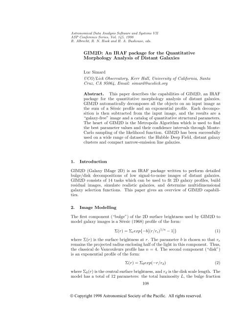
Figure 1. Left: HST/WFPC2/WF4 4400 seconds image of a region 

in the z = 0.4 cluster CL0024+16. Right: GIM2D residual image. 157 

objects were fitted, and galaxies which were too close to the edge of 

the image were not analyzed. 

1996). It was also found that a number of HDF galaxies have surface brightness 

profiles with Sérsic index n ≤ 1. Some of them exhibit double exponential 

profiles which can be easily mistaken for pure bulge systems. However, these 

systems have spectra resembling those of late-type star-forming galaxies. Other 

HDF objects are best-fitted with a single n




Grid OCL : A Graphical Object Connecting Language 

I. J. Taylor 1 

Department of Physics and Astronomy, University of Wales, College of 

Cardiff, PO BOX 913, Cardiff, Wales, UK, Email: 

Ian.Taylor@astro.cf.ac.uk 

B. F. Schutz 2 

Albert Einstein Institute, Max Planck Institute for Gravitational 

Physics, Schlaatzweg 1, Potsdam, Germany. Email: 

schutz@aei-potsdam.mpg.de 

Abstract. In this paper, we present an overview of the Grid OCL 

graphical object connecting language. Grid OCL is an extension of Grid, 

introduced last year, that allows users to interactively build complex data 

processing systems by selecting a set of desired tools and connecting them 

together graphically. Algorithms written in this way can now also be run 

outside the graphical environment. 


Signal-processing systems are becoming an essential tool within the scientific 

community. This is primarily due to the need for constructing large complex 

algorithms which would take many hours of work to code using conventional 

programming languages. Grid OCL (Object Connecting Language) is a graphical 

interactive multi-threaded environment allowing users to construct complex 

algorithms by creating an object-oriented block diagram of the analysis required. 

2. An Overview 

When Grid OCL is run three windows are displayed. A ToolBox window, a Main- 

Grid window and a Dustbin window (to discard unwanted units). Figure 1 shows 

the ToolBox window which is divided into two sections. The top section shows 

the available toolboxes (found by scanning the toolbox paths specified in the 

Setup menu) and the bottom shows the selected toolbox’s contents. Toolboxes 

(and associated tools) can be stored on a local server or distributed throughout 

several network servers. Simply adding the local or http address in the toolbox 

and tool path setup allows on-the-fly access to other people’s tools. 

1 A post doctoral programmer at Cardiff who has been developing Grid OCL since January 1996. 

2 Professor Schutz is a Director of the Albert Einstein Institute, Potsdam 

112 


Grid OCL : A Graphical Object Connecting Language 113 

Figure 1. Grid OCL’s ToolBox window. Toolboxes can be organised 

in a similar way to files in a standard file manager. 

Units are created by dragging them from the ToolBox window to the desired 

position in the MainGrid window and then connected together by dragging from 

an output socket on a sending unit to an input socket of the receiving unit. The 

algorithm is run by clicking on the start button (see Figure 2), in a single step 

fashion (i.e., one step at a time) or continuously. 

3. New Features and Extensions 

Groups of units can now be saved along with their respective parameters. Such 

groups can also contain groups, which can contain other groups and so on. This 

is a very powerful feature which allows the programmer to hide the complexity 

of programs and use groups as if they were simply units themselves. Many 

improvements have been made to the graphical interface, including compacting 

the look and style of the toolbox, adding a snap-to cable layout and many more 

informative windows. The major change however, is that now Grid consists of 

an object connecting language (OCL) and a separate user interface. This means 

that the units can be run from within the user interface or as a stand-alone 

program. 

Collaborators are working on tools for various signal and image problems, 

multimedia teaching aids and even to construct a musical composition system. 

Currently, in our new release we have toolboxes for various signal processing 

procedures, animation and a number of image processing/manipulation routines, 

text processing tools e.g., find and replace, grep and line counting recursively 

through subdirectories, mathematical and statistical units, a general purpose 

mathematical calculator (see next section) and a number of flexible importing 

and exporting units.

114 Taylor and Schutz 

4. MathCalc 

Figure 2. A snapshot of Grid OCL’s programming window. 

The MathCalc unit interprets, optimises and evaluates arithmetic expressions 

using stream-oriented arithmetic. It recognises a large number of functions and 

constants. It can be used to evaluate scalar expressions, to process input data 

sets, or to generate output data sets. All calculations are performed in doubleprecision 

real arithmetic. 

Stream-oriented arithmetic can be defined as the application of an arithmetic 

expression to each element of a stream independently. Thus, if B is 

the sequence b1,b2, .., bn, then the function sin(B) evaluates to the sequence 

sin(b1),sin(b2), ..., sin(bn). MathCalc distinguishes between constants and sequences 

or sets. Sets (data sets) are sequences of numbers and constants are 

single numbers, essentially sequences of length 1. In a MathCalc expression the 

two can be mixed very freely, with the restriction that all sequences must have 

the same length. Sequences or constants can be obtained from the input nodes of 

the MathCalc unit. The example given in the MainGrid window (see Figure 2) 

demonstrates the flexibility of the MathCalc unit. 

The first MathCalc unit creates a 125 Hz sine wave by using the equation 

sin(((sequence(512) ∗ 2) ∗ PI) ∗0.125) where the sample rate is 1kHz (Math- 

Calc will optimise this to (2*PI*0.125) * sequence(512)). This is then transformed 

into a SampleSet type by adding its sampling frequency (i.e., 1 kHz). 

The second MathCalc unit adds Gaussian noise to its input (i.e., by typing 

gaussian(512)+#0s). The #0 means node 0 and the s meansthatitisasequence 

as opposed to a c which would a constant. The resultant amplitude 

spectrum (FFTASpect) is shown from Grapher1 (see Figure 3). 

Once the signal is displayed, it can be investigated further by using one of 

the Grapher’s various zooming facilities. Zooming can be controlled via a zoom 

window which allows specific ranges to be set or by simply using the mouse to 

drag throughout the image. For example, by holding the control key down and 

dragging down the image is zoomed in vertically and by dragging across from 

left to right zoomed in horizontally. The reverse operations allow zooming out. 

Also once zoomed in, by holding the shift key and the control key down the 

mouse can be used to move around the particular area you are interested in. We 

also have another powerful zooming function which literally allows the user to 

drag to the position of interest and the image will zoom in accordingly.

Grid OCL : A Graphical Object Connecting Language 115 

Figure 3. Grapher1’s output: any grapher can simultaneously display 

many signals each with its own colour and line style. 

5. Grid OCL : Past and Present 

Grid originated from an implementation of the system using C++ and Inter- 

Views (Taylor & Schutz 1995) but was abandoned in early 1996. Version two 

(Taylor & Schutz 1996) was written using the Java Development Kit, JDK 1.0.2 

but this was updated in order to be compatible with the new JDK 1.1.x kit. 

We also re-implemented the base classes and to create OCL. The most recent 

version of Grid OCL (in November 1997) is a late alpha and goes by a different 

name (Triana OCL 4 ). Triana OCL will be entering its beta testing stage early 

next year followed by a final version shortly after. We are in the process of being 

able to provide a commercial version of the software for which support can be 

given. None-the-less we will always provide it in a free downloadable from the 

WWW with a certain time limit (3 or 4 months). Our main goal is to create a 

very wide user base. 

References 

Taylor, I. J. & Schutz, B. F. 1995, The Grid Musical-Signal Processing System, 

International Computer Music Conference, 371 

Taylor, I. J. & Schutz, B. F. 1996, The Grid Signal Processing System. in ASP 

Conf. Ser., Vol. 125, Astronomical Data Analysis Software and Systems 

VI,ed.GarethHunt&H.E.Payne(SanFrancisco:ASP),18 

4 http://www.astro.cf.ac.uk/Triana/




GUI-fying and Documenting your Shell Script 

Peter. J. Teuben 1 

Astronomy Department, University of Maryland, College Park, MD 

20742, Email: teuben@astro.umd.edu 

Abstract. 

We describe a simple method to annotate shell scripts and have a 

preprocessor extract a set of variables, present them to the user in a 

GUI (using Tcl/Tk) with context sensitive help, and run the script. It 

then becomes also very easy to rerun the script with different values of 

the parameters and accumulate output of different runs in a set of user 

defined areas on the screen, thereby generating a very powerful survey 

and analysis tool. 


Scripting languages have often been considered the glue between individual applications, 

and are meant to achieve a higher level of programming. 

When individual applications are (tightly) integrated into the scripting language, 

this offers very powerful scripts, fully graphical user interfaces and a 

result sometimes indistinguishable from applications. A recent example of this 

is the glish shell in AIPS++ (Shannon 1996). But of course the drawback of this 

tight integration is that applications are not always easily accessible to scripts 

that do not (or cannot) make use of the environment the scripting language was 

meant for. 

Apart from the black art of handcoding, one of the traditional methods 

to add a GUI to an application is using automatic GUI builders. This has 

the advantage that application code and user interaction code are more cleanly 

separated, but this sometimes also limits the flexibility with which the code can 

be written. 

This paper presents a simple implementation where the style of the underlying 

application is batch oriented, and in fact can be written in any language. 

The user interface must be cleanly defined in a set of parameters with optional 

values (e.g., named “keyword=value” pairs). Once the input values have been 

set, the application can be launched, results can be captured and presented in 

any way the script or application decides. 

2. Tcl/Tk: TkRun 

The GUI that is created will provide a simple interface to a program that is 

spawned by the GUI. This program must have a well defined Command Line 

116 


GUI-fying and Documenting your Shell Script 117 

Interface (CLI), in the current implementation a “keyword=value” interface. 

Equally well, a Unix-style “-option value” could have been used (cf. Appleton’s 

parseargs package). The GUI builder, a small 600 line C program called tkrun, 

scans the script for special tags (easily added as comments, which automatically 

make the script self-documenting), and creates a Tcl/Tk script from which the 

shell script itself (or any application of choice with a specified CLI) can be 

launched (see Figure 2 for a schematic). 

The added power one gets with this interface builder is the simplified reexecution 

of the script, which gives the user a powerful tool to quickly examine 

a complex parameter space of a particular problem. 

The input script must define a set of parameters, each with a keyword, an 

optional initial value, a widget style, usage requirements and one line help. The 

keyword widget style can be selected from a small set of input styles that standard 

Tcl/Tk provides (such as generic text entry, file browsers, radio buttons, 

sliders etc.) 

The current implementation has been tested under Tcl/Tk 7.6 as well as 

8.0, but is expected to move along as Tcl/Tk is developed further. For example 

a more modern widget layout technique (grid instead of pack) should be used. 

Also keywords cannot have dependencies on each other, for example it would be 

nice to “grey out” certain options under certain circumstances, or allow ranges 

of some keywords to depend on the settings of others. 

3. Sample Script: testscript 

Here is an example header from a C-shell script with which Figure 1 was made. 

Note that the script must supply a proper “keyword=value” parsing interface, 

as was done with a simple foreach construct here. The latest version of tkrun 

is available through the NEMO 1 package. 

#! /bin/csh -f 

# :: define basic GUI elements for tkrun to extract 

#> IFILE in= 

#> OFILE out= 

#> ENTRY eps=0.01 

#> RADIO mode=gauss gauss,newton,leibniz 

#> CHECK options=mean,sigma sum,mean,sigma,skewness,kurtosis 

#> SCALE n=1 0:10:0.01 

# :: some one liners 

#> HELP in Input filename 

#> HELP out Output filename (should not exist yet) 

#> HELP eps Initial (small) step 

#> HELP mode Integration Method 

#> HELP options Statistics of residuals to show 

#> HELP n Order of polynomial 

# :: parse named arguments 

foreach a ($*) 

set $a 

end 

1 http://www.astro.umd.edu/nemo/

118 Teuben 

Figure 1. With the command “tkrun testscript” the upper panel 

is created, providing a simple interface to the “key=val” command line 

interface of the script testscript (see below). The lower panel is a 

standard Tcl/Tk filebrowser that can be connected to keywords that 

are meant to be files. See Figure 2 for a schematic diagram explaining 

the interaction between the different programs and scripts. 

# :: actual start of code 

echo TESTSCRIPT in=$in out=$out eps=$eps mode=$mode options=$options n=$n 

# :: legacy script can be inserted here or keyword 

# :: values can be passed on to another program 

Acknowledgments. I would like to thank Frank Valdes and Mark Pound 

for discussing some ideas surrounding this paper, and Jerry Hudson for his 

Graphics Command Manager FLO. 

References 

Appleton, Brad (parseargs, based on Eric Allman’s version)

tkrun testscript 

GUI-fying and Documenting your Shell Script 119 

testscript 

#! /bin/csh -f 

#> IFILE 

# tags 

in= 

#> ENTRY eps= 

... 

... 

# code: 

#! /bin/wish -f 

... 

lappend args .... 

exec testscript $args 

... 

testscript.tk 

testscript in=... out=... eps=... .... 

in: 

wish -f testscript.tk 

RUN 

Figure 2. Flow diagram: The command tkrun scans the C-shell 

script testscript (top left) for keywords and the Tcl/Tk script 

testscript.tk (bottom left) is automatically written and run. It 

presents the keywords to the user in a GUI (on the right, see Figure 

1 for a detailed view) ), of which the “Run” button will execute 

the C-shell code in the script testscript. 

Judson, Jerry (FLO: a Graphical Command Manager) 

Ousterhout, John, 1994, Tcl and the Tk Toolkit, Addison-Wesley 

Shannon, P., 1996, in ASP Conf. Ser., Vol. 101, Astronomical Data Analysis 

Software and Systems V, ed. George H. Jacoby & Jeannette Barnes (San 

Francisco: ASP), 319 

Teuben, P.J., 1995, in ASP Conf. Ser., Vol. 77, Astronomical Data Analysis 

Software and Systems IV, ed. R. A. Shaw, H. E. Payne & J. J. E. Hayes 

(San Francisco: ASP), 398 

eps:




The Mosaic Data Capture Agent 

Doug Tody and Francisco G. Valdes 

IRAF Group, NOAO 1 , PO Box 26732, Tucson, AZ 85726 

Abstract. The Mosaic Data Capture Agent (DCA) plays a central role 

in connecting the raw data stream from the NOAO CCD Mosaic controller 

system to the rest of the data handling system (DHS). It is responsible for 

assembling CCD data from multiple readouts into a multiextension FITS 

disk file, for supplying a distributed shared image to real-time elements 

of the DHS such as the Real-Time Display (RTD), and for feeding data 

to the IRAF-based data reduction agent (DRA). 

1. Overview 

A brief design of the data handling system (DHS) for the NOAO CCD Mosaic 

Camera 2 was presented earlier (Tody, 1997). It is based on a message bus 

architecture (Tody, 1998) that connects the various components of the DHS. 

One such component is the data capture agent (DCA). The DCA receives streams 

of readout data from the acquisition system and builds a data object which is 

shared by other components of the DHS. The image data is stored on disk as a 

multiextension FITS file (MEF) (see Valdes 1997b). 

The DCA is a general purpose network-based data service, using the message 

bus as the network interface. It receives request messages of various types 

and, through an event loop, dispatches each request to the appropriate event 

handler. The request message types currently implemented in the DCA are for 

control, setting or querying server parameters, readout status, data format configuration, 

and writing header and pixel data. In addition to servicing client 

requests, the DCA can broadcast messages to inform clients of the status of the 

DCA during readout. 

The major subsystems of the DCA at present are the message bus interface, 

an event loop and event handlers for processing message requests, a distributed 

shared object implementation, a keyword database system, the TCL interpreter, 

and a TCL-based keyword translation module. 

1 National Optical Astronomy Observatories, operated by the Association of Universities for 

Research in Astronomy, Inc. (AURA) under cooperative agreement with the National Science 

Foundation. 

2 http://www.noao.edu/kpno/mosaic/ 

120 


2. DCA User Interface 

The Mosaic Data Capture Agent 121 

The DCA may be started by issuing a command at the host level, or invoked as a 

service via the message bus. This can occur during login to an observing account, 

using a window manager menu, or by interactively issuing a user command. The 

command invocation can include DCA server parameters which can also be set 

or reset after invocation via messages. 

The DCA automatically connects to the message bus when it is started. 

The runtime operation of the DCA is monitored and controlled by clients via 

the message bus. In the Mosaic system there are two clients; the data feed 

client (DFC) and the DCA console client (DCAGUI). In general any number 

of clients can access the DCA. Multiple data feed clients or GUIs can be active 

simultaneously. 

The DCA console client has a graphical user interface based on the IRAF 

Widget Server (Tody, 1996). It can send control and parameter messages to the 

DCA and act on messages broadcast by the DCA, e.g., to display the readout 

status. Currently the DCAGUI executes an autodisplay command for real time 

display during readout (see Valdes, 1998) and a post-processing command for 

logging, archiving or other operations once the readout ends. 

3. The Readout Sequence 

An observation readout is driven by a sequence of DCA message requests. A 

readout sequence is initiated by the DFC with a message that includes a unique 

sequence number. Once a readout has started, each subsequent message associated 

with that readout must be tagged with the sequence number for that 

readout. Multiple readouts can be simultaneously in progress. Each readout 

sequence has a separate context identified by its sequence number. 

When a readout sequence is initiated the DCA creates a new image-class 

distributed shared object (DSO). The DFC passes information about the size and 

structure of the object (such as the number of image extensions), allowing the 

DCA to configure the DSO. At this point the DFC can begin sending pixel and 

header messages. At image creation time the DCA broadcasts a message so that 

clients like the DCAGUI can access it if desired. Currently the DCAGUI uses 

this to initiate an interim real-time display. 

When the readout is completed the DCA executes a keyword translation 

module (KTM), an externally supplied, interpreted TCL script which converts 

detector specific information into standard header keywords. After the KTM 

finishes the DCA and DSO format the output keywords, write them to the 

image headers, and generation of the new image DSO is complete. The DCA 

broadcasts a message when the DSO is complete which can be used to trigger 

post-processing of the data. 

3.1. Pixel Messages 

The pixel data messages contain blocks of raw, unprocessed detector pixel data 

organized into one or more streams, one for each CCD amplifier. Each stream 

directs pixels to a region of an output image extension. This structure allows 

the data block to simultaneously contain data for several different regions and

122 Tody and Valdes 

the data can be arbitrarily interleaved, encoded, flipped, or aliased. Each block 

of data is processed asynchronously but the client can send a synchronization 

request periodically to check the output status. 

3.2. Keyword Messages 

The DCA receives header information via the message bus. This information 

consists of blocks of keywords organized into named, detector specific keyword 

groups. The keywords are stored in keyword databases (an internal random access 

data structure), one per keyword group. The set of keyword group names is 

arbitrary. Some examples for the NOAO Mosaic are ICS for instrument control 

system, TELESCOPE for telescope, and ACEBn for Arcon controller information 

for controller n. 

The Arcon controller system for the NOAO Mosaic consists of a set of 

Arcon controllers each of which can readout one or more amplifiers. The current 

system has four controllers each reading out two CCDs using one amplifier per 

CCD. Thus there can be controller information for the whole system, for each 

controller, and for each amplifier readout. 

A keyword database library handles creation and maintenance of the keyword 

database. Note that keyword information does not necessarily have to 

come only from the DFC, the current mode of operation for the NOAO Mosaic. 

Other schemes are possible. 

4. Keyword Translation Module 

The keyword translation module (KTM) is a TCL script called by the DCA at 

the end of a readout, once all raw header information has been received. The 

purpose of the KTM is to create the keywords for the global and extension 

headers. The KTM is passed a list of input keyword database descriptors and 

it returns a list of output keyword database descriptors, one for each header. 

The DCA TCL interpreter provides special TCL commands for manipulating 

(creating, accessing, searching, etc.) the keyword databases. When the KTM 

finishes the DCA, via the DSO, writes the keywords in the returned output 

keyword databases to the output MEF FITS file. 

The KTM performs a variety of transformations on the input keywords. A 

keyword can be copied verbatim if no change is desired. The keyword name or 

comment may be changed without changing the value. New keywords can be 

added with static information and default values may be supplied for missing 

keywords. The KTM can compute new keywords and values from input keywords. 

Identical keywords in each extension may be merged into a single keyword 

in the global header. The KTM can detect incorrect or missing keywords and 

print warnings or errors. 

Two examples from the keyword translation module for the NOAO CCD 

Mosaic follow. 

1. The data acquisition system provides the keywords DATE-OBS and UT- 

SHUT giving the UT observation date in the old FITS date format 

(dd/mm/yy) and the UT of the shutter opening. The KTM converts these

The Mosaic Data Capture Agent 123 

to TIME-OBS, MJD-OBS, OBSID, and the new Y2K-compliant FITS date 

format. 

2. The KTM determines on which telescope the Mosaic Camera is being 

used and writes the WCS scale, orientation, and distortion information 

previously derived from astrometry calibrations for those telescopes. The 

coordinate reference point keywords, CRVAL1 and CRVAL2, are computed 

from the telescope right ascension and declination keywords. 

5. Distributed Shared Objects and Distributed Shared Images 

An important class of message bus component is the distributed shared object 

(DSO). DSOs allow data objects to be concurrently accessed by multiple clients. 

The DSO provides methods for accessing and manipulating the data object and 

locking facilities to ensure data consistency. DSOs are distributed, meaning 

that clients can be on any host or processor connected to the message bus. In 

the case of the Mosaic DHS, the principal DSO is the distributed shared image 

which is used for data capture, to drive the real-time display, and for quick 

look interaction from within IRAF. The distributed shared image uses shared 

memory for efficient concurrent access to the pixel data, and messaging to inform 

clients of changes to the image. 

The current version of the DCA does not implement the full distributed 

shared image object. Instead it implements a mapped image file. The image 

being created appears as a valid FITS multiextension file immediately after the 

configuration information is received from the DFC. This allows applications 

to examine the file while the readout is in progress. An example of this is the 

interim display routine that loads a display server frame buffer as the pixel data 

is recorded, giving a simple real-time display capability. 

6. Current Status and Future Developments 

A version of the Data Capture Agent is in production use at two telescopes on 

Kitt Peak with the NOAO CCD Mosaic Camera. The flexibility of the message 

bus architecture is used to provide two modes of operation. The standard mode 

uses two machines connected by fast Ethernet. One machine supports the observing 

user interface and the interface to the controller system. A DFC running 

on this host writes to the message bus and the DCA runs on another machine 

(with a different OS) where the exposures are written to disk and the quick look 

interaction and any post-processing are done. The second mode is a fallback 

in case the second computer fails. The DCA can simply be run on the same 

machine as the UI and controller interface. 

Future developments will complete the distributed shared object and console 

client and add other clients such as the real-time display (Tody, 1997) and 

data reduction agent (Valdes 1997a). 

The design of the DCA (and the whole DHS based on the message bus 

architecture) is open, flexible, and efficient. It can be used with many data 

acquisition systems at a variety of observatories. All that is needed is to write a 

data feed client to connect to the message bus and a keyword translation module

124 Tody and Valdes 

appropriate for the data. Currently the lower level messaging system is based 

on the Parallel Virtual Machine (PVM) library but this can be replaced in the 

future with other messaging systems such as CORBA. 

References 

Tody, D. 1996, in ASP Conf. Ser., Vol. 101, Astronomical Data Analysis Software 

and Systems V, ed. George H. Jacoby & Jeannette Barnes (San Francisco: 

ASP), 89 

Tody, D. 1997, in ASP Conf. Ser., Vol. 125, Astronomical Data Analysis Software 

and Systems VI, ed. Gareth Hunt & H. E. Payne (San Francisco: ASP), 

451 

Tody, D. 1998, this volume 

Valdes, F. 1997a, in ASP Conf. Ser., Vol. 125, Astronomical Data Analysis 

Software and Systems VI, ed. Gareth Hunt & H. E. Payne (San Francisco: 

ASP), 455 

Valdes, F. 1997b, in ASP Conf. Ser., Vol. 125, Astronomical Data Analysis 


ASP), 459 

Valdes, F. 1998, this volume




Packaging Radio/Sub-millimeter Spectral Data in FITS 

Zhong Wang 

Smithsonian Astrophysical Observatory, Cambridge, MA 02138 U.S.A. 

Email: zwang@cfa.harvard.edu 

Abstract. We report on an experiment to incorporate the multiple 

extension FITS file format in building data processing software for spectroscopic 

observations in radio and millimeter-submillimeter wavelengths. 

By packaging spectral header information into table extensions and the 

actual spectral data into either table or image extensions, this approach 

provides a convenient and effective way to organize large amount of spectroscopic 

data, especially for pipeline-like processing tasks. Tests conducted 

based on a software package developed for the SWAS mission have 

demonstrated this to be a viable alternative to the conventional ways of 

organizing spectral data at these wavelengths. 

1. Introduction: Characteristics of Submillimeter Spectral Data 

Historically, spectral data were taken roughly one spectrum at a time, and most 

existing data formats reflect such a methodology. The traditional ways in which 

FITS can be used for spectral data are less than adequate in meeting the needs 

of a new generation of instruments that produce large amount of relatively homogeneous 

data, which nevertheless need to be reduced individually. A set of 

more efficient, better streamlined reduction procedures are necessary, which in 

turn require more careful considerations in data packaging. This is particularly 

important for projects that adopt non-interactive, pipeline-style data processing 

as their primary mode of operation. 

The SWAS 1 (Submillimeter Wave Astronomy Satellite) mission is essentially 

a small orbiting radio telescope working at relatively high (about 500 

GHz) frequencies (Wang 1995). It is designed to make simultaneous spectroscopic 

measurements at several sub-mm line wavelengths that are inaccessible 

from the ground. The spectral data have some special characteristics: 

• Integration time for each individual “scan” is set to be short (on the order 

of a few seconds). High signal-to-noise ratios are achieved by co-adding a 

large number of such scans at the data processing stage; 

1 Details of the SWAS mission can be found on the internet in SAO’s SWAS homepage at 

http://cfa-www.harvard.edu/cfa/oir/Research/swas.html 

125 


126 Wang 

• Because of the noise properties and frequency shifts with time (due to the 

motion of the spacecraft as well as instrumental drifts), individual scans 

need to be calibrated separately before co-adding; 

• More than one spectral band is recorded at any given time, thus a complete 

dataset consists of spectra of several different wavelength ranges from independent 

detectors. Yet they are of the same source and are taken under 

very similar observing conditions; 

• Observations are broken up into individual “segments” each lasting typically 

30–40 minutes. During each segment, many spectroscopic scans 

(aside from calibration data) are simple repeats under nearly identical 

conditions, and therefore share values of many header parameters with 

only slight variations (drifts). 

The data reduction plan for the mission calls for a highly efficient pipeline 

processing scheme in which a large amount of spectroscopic data can be sorted, 

selected, calibrated and co-added based on some user-changeable criteria. All 

processing operations have to be recorded and traceable, and are preferably done 

with minimal human intervention. 

2. Software Approach: Packaging Data in FITS 

We have selected IRAF as our primary programming platform for the SWAS 

pipeline software, and use FITS as the main format for our data product. However, 

to store individual scan data in the conventional one- (single spectrum) or 

two-dimensional (“multispec” or echelle) format would be very inefficient and 

even confusing. 

Our approach is to make use of the BINTABLE and IMAGE extensions of 

FITS and store spectral header and pixel data in these two types of extensions 

in a single FITS data file. The basic rules we adopted are: 

• Each FITS file corresponds to a specific time interval of data taking (an 

observing segment). It contains a single BINTABLE extension and (optionally) 

several IMAGE extensions. It has a conventional header section 

containing some none-time-variable, shared parameters of the spectra; 

• The table extension has one row per spectral scan taken, and stores all of 

the time-variable spectral header information corresponding to that scan 

(i.e., time, coordinates, frequency, noise statistics, etc); 

• The pixel data of the spectrograph output (the spectrum itself) can be 

stored in one of two ways: they can either be individual “array elements” 

of a table row, or an image row similar to the two-dimensional arrays used 

to save Echelle and multi-fiber spectra in the optical. 

In case of using variable-length, vector (array) columns to store pixel data, 

a table row can have more than one array element, each representing data 

of a separate spectral band. The length of an array element is the number 

of pixels in a spectrum of that band.

Packaging Radio/Sub-millimeter Spectral Data in FITS 127 

In case of images, each image row corresponds to a row in the header 

parameter table. The number of columns of the image is the same as the 

number of pixels in a spectrum. There can be multiple image extensions 

in each data file, with different extensions representing data of different 

spectral bands. 

The choice between using the table extension of FITS alone versus using 

table plus image extensions depends on the actual application. In principle, saving 

everything in a single table is structurally more appealing and efficient, but 

not many existing software tools can accept variable-length vector column FITS 

tables — which means more development work for basic tools. On the other 

hand, making use of 2-D images can facilitate data inspection procedures with 

various tools that examine FITS images. Its shortcoming is that information 

about a single spectrum is saved in two or more extensions, requiring care in 

managing them. 

3. Advantages and Efficiency Gains 

Given the lack of a widely-accepted standard in formatting a largely homogeneous 

spectroscopic dataset, we find the packaging using FITS extensions to be 

a viable alternative to the conventional ways in which spectral data are saved: 

• It provides a convenient way to organize, sort, edit, monitor and visualize 

the large spectral dataset (much of it is done with existing tools within 

IRAF or those directly working with FITS), while preserving all the essential 

information of each individual spectrum; 

• The programming of calibration tasks to process a relatively large, nearlyhomogeneous 

dataset is very much simplified. In particular, the spectral 

header parameters can be processed either independently or as table 

columns. It also means that, for example, a subset of the header parameters 

of a large number of spectra can be easily manipulated without even 

accessing the actual pixel data; 

• The efficiency of data processing is clearly enhanced. Since spectral pixel 

data are always processed as arrays, the fractional time taken by file I/Os 

and data buffering is substantially reduced when, for example, those data 

are accessed as part of an image. 

Many of the existing software tools that deal with FITS table and image 

data are readily available for use with these new data files, sometimes with minor 

modifications. This can significantly save the programming effort and shorten 

the software development cycle. 

4. Comments and Future Work 

Despite the considerable merits of this approach, some problems remain to be 

addressed, and we are working on future enhancement of our software.

128 Wang 

One of the main problems is the interface with existing software tools (such 

as visualization tools from certain existing tools packages). In practice, we were 

able to partly circumvent this shortcoming by writing customized interfaces, 

but the solutions are not always satisfactory. It appears that if a tabular style 

file format is deemed sufficiently important, a more fundamental (kernel-level) 

interface for spectral data in FITS should be developed. 

The approach described in this paper is an explorative step in enhancing the 

use of FITS, especially in taking advantage of the multiple extension development 

and the use of vector columns in FITS tables. With the rapid advancement 

in database and data warehousing technology, one would ideally like to have a 

more rigorous database-like framework to deal with the management of the observational 

data. This, however, needs to be balanced with the requirement 

of cost-effective and quick prototyping of many projects’ practical applications. 

The latter often means maximizing the use of existing software tools and adopting 

conventional approaches. The multiple extension FITS adopted by the community 

and being incorporated by NOAO and STScI’s IRAF teams (e.g., Zarate 

& Greenfield 1996, Zarate 1998) and other software groups is an important and 

innovative development, which preserves the usefulness of many old tools while 

allowing new methods to be tested for astronomical data applications. We believe 

that more efforts are needed in exploring ways to take full advantage of 

this very useful data format. 

References 

Wang, Z. 1995, in ASP Conf. Ser., Vol. 77, Astronomical Data Analysis Software 

and Systems IV, ed. R. A. Shaw, H. E. Payne & J. J. E. Hayes (San 


Zarate, N. & Greenfield, P. 1996, in ASP Conf. Ser., Vol. 101, Astronomical 

Data Analysis Software and Systems V, ed. George H. Jacoby & Jeannette 

Barnes (San Francisco: ASP), 331 

Zarate, N. 1998, this volume 

Acknowledgments. We are grateful to Phil Hodge and Nelson Zarate for 

their help in the software development discussed in this paper. Dr. Matthew 

Ashby has participated in implementation and testing of the SWAS software.




The IDL Wavelet Workbench 

M. Werger 

Astrophysics Division, Space Science Department of ESA, ESTEC, 2200 

AG Noordwijk, The Netherlands, EMail: mwerger@astro.estec.esa.nl 

A. Graps 

Stanford University, Center for Space Science and Astrophysics, HEPL 

Annex A210, Stanford, California, 94305-4085 EMail: 

amara@quake.stanford.edu 

Abstract. Progress in the development of the 1996 release of the IDL 

Wavelet Workbench (WWB) is shown. The WWB is now improved in 

several ways, among them are: (1) a smarter GUI which easily directs the 

user to the possibilities of the WWB, (2) the inclusion of more wavelets, 

(3) the enhancement of the input and output modules to provide a better 

interface to the input and output data and (4) the addition of more 

analysis methods based on the wavelet transform. 


One of the most advanced packages for wavelet analysis is probably Wavelab 1 

written for MATLAB. New insights have been gained in many other fields by 

applying wavelet data analysis, thus it was a reasonable task for us in astronomical 

research to translate most of the code from the Wavelab package into 

IDL (Interactive Data Language, by Research Systems, Inc.). IDL was chosen 

because of its wide-spread availability in the astronomical community and because 

of its development environment. The last official version of the so-called 

IDL Wavelet Workbench (WWB) was in the Spring of 1996. It has been made 

publicly available at the ftp site of Research Systems, Inc. 2 . 

2. The 1996 version of IDL 

The 1996 version of the WWB consists of 111 different modules with approximately 

10,000 lines of code in total. Approximately all modules have been 

written or translated from MATLAB code into IDL by AG. The 1996 version 

can be run either from the IDL command line or from a graphical user interface 

(GUI). 

1 http://stat.stanford.edu/ ∼ wavelab/ 

2 ftp://ftp.rsinc.com/ 

129 


130 Werger and Graps 

The WWB is written in a highly modularized way to be easily maintained 

and improved. In the 1996 version, COMMON blocks are used to store important 

variables for the different routines. These COMMON blocks can be set 

also from the command line. Therefore, it is possible to use the WWB as a 

stand-alone package and also as a library to supplement ones own IDL routines. 

The 1996 WWB provides simple input and output routines. Its analysis 

and plotting libraries are sophisticated and employ most of the typical methods 

used in wavelet analysis like the Discrete Wavelet Transform, Multiresolution 

Analysis, Wavelet Packet Analysis, Scalegram, andScalogram. In addition, the 

1996 WWB offers typical routines for de-noising and compression of one- and 

two-dimensional data. The available set of wavelets is restricted up to four important 

families: the Haar-wavelet and the families of the Daubechies-wavelets, 

Coiflets, and Symmlets. 

3. Current Developments 

The 1996 release the IDL WWB has been widely used for different tasks such 

as pattern detection, time-series analysis and de-noising of data. A lot of useful 

routines have been added to the WWB since 1996, or they are foreseen to be 

included. 

• The current version makes use of the most recent changes to IDL (version 

5.0.2); now WWB uses pointers to handle arbitrary data arrays. Also, the 

WWB command line interface and the GUI may be used at the same time. 

• The GUI has been simplified; now it includes more possibilities, but with 

an easier interface and a less complicated dialog structure. 

• All necessary variables are now kept in two IDL data structures, those 

variables also may be set from the command line. 

• The data input portion of the WWB has been upgraded to handle FITSfiles; 

the output portion of WWB has been upgraded so that one can use 

the GUI to set PostScript output. 

• More analysis routines are now available. In additional to the forward 

DWT, now the backward DWT (IWT ) has been included to show possible 

differences between the original and transformed data. A continuous 

wavelet transform using the Gauss, Sombrero, and Morlet wavelets has 

been added also. 

• The capabilities for time-series analysis has been greatly enhanced by 

adding wavelets and routines which improve period detection. For example, 

a routine has been added for detecting periods in unevenly-sampled 

time-series, and eleven new wavelet filters are provided. 

• The computations can now allow datasets more than 32767 points long. 

• Plotting capabilities of the Scalogram have been improved.

The IDL Wavelet Workbench 131 

• For a better understanding of the wavelet transform, a GUI for manipulating 

specific wavelet coefficients has been included. This greatly improves 

the learning and analyzing process. 

4. Future Plans 

There are some future plans for integrating capabilities to analyze multidimensional 

data and adding additional routines. Suggestions and contributions from 

the user community are greatly welcome. 

Acknowledgments. The 1996 WWB has been partly funded by RSI, Inc.




IRAF Multiple Extensions FITS (MEF) Files Interface 

Nelson Zarate 

National Optical Astronomy Observatories 

Tucson, AZ 85719 (zarate@noao.edu) 

Abstract. The Multiple Extension FITS (MEF) file interface is an 

IRAF library providing facilities for general file operations upon FITS 

multi-extension files. The MEF library has been used as the basis for a 

set of new IRAF tasks providing file level operations for multi-extension 

files. These operations include functions like listing extensions, extracting, 

inserting, or appending extensions, deleting extensions, and manipulating 

extension headers. MEF supports extensions of any type since it 

is a file level interface and does not attempt to interpret the contents of 

a particular extension type. Other IRAF interfaces such as IMIO (the 

FITS image kernel) and STSDAS TABLES are available for dealing with 

specific types of extensions such as the IMAGE extension or binary tables. 


The Multiple Extensions FITS (MEF) interface consists of a number of routines 

to mainly read a FITS Primary Data Unit or an Extension Unit and manipulate 

the data at a file level. It is up to the application to take care of any details 

regarding data structuring and manipulation. For example, the MEF interface 

will read a BINTABLE extension and give to the calling program a set of parameters 

like dimensionality, datatype, header buffer pointer and data portion 

offset from the beginning of the file. 

Currently the routines available to an SPP program are: 

• mef = mef_open (fitsfile, acmode, oldp) 

• mef_rdhdr (mef, group, extname, extver) 

• mef_rdhdr_exnv (mef, extname, extver) 

• mef_wrhdr (mefi, mefo, in_phdu) 

• [irdb]val = mefget[irdb] (mef, keyword) 

• mefgstr (mef, keyword, outstr, maxch) 

• mef_app_file (mefi, mefo) 

• mef_copy_extn (mefi, mefo, group) 

132 


IRAF Multiple Extensions FITS (MEF) Files Interface 133 

• mef_dummyhdr (fd, hdrfname) 

[irdb]: int, real, double, boolean. 

2. Initializing Routine 

2.1. mef = mef open (fitsfile, acmode, oldp) 

Initializes the MEF interface. Should be the first routine to be called when 

performing operations on FITS files using this set of routines. Returns a pointer 

to the MEF structure. 

fitsfile Pathname to the FITS file to be open. The general syntax is: 

dir$root.extn[group] 

• dir: Directory name where the file resides 

• root: Rootname 

• extn: (optional) Extension name — can be any extension string 

• group: Extension number to be opened 

The ‘[group]’ string is optional and is not part of the disk filename. It is 

used to specified which extension number to open. The extension number 

is zero based — zero for the primary extension, 1 for the first extension, 

and so on. 

acmode The access mode of the file. The possible values are: 

READ ONLY, READ WRITE, APPEND, NEW FILE 

oldp Not used. Reserve for future use. 

3. Header Routines 

3.1. mef rdhdr (mef, group, extname, extver) 

Read the FITS header of a MEF file that matches the EXTNAME or EXTVER 

keyword values or if not specified, read the extension number ‘group’. If no 

extension is found an error is posted. After reading the header the file pointer 

is positioned at the end of the last data FITS block (2880 bytes). 

mef The MEF pointer returned by mef open. When the routine returns, all 

of the elements of the MEF structure will have values belonging to the 

header just read. 

group The extension number to be read — zero for the Primary Data Unit, 1 

for the first extension, and so on. If you want to find out an extension by 

the value of extname and/or extver then ‘group’ should be -1. 

extname The string that will match the EXTNAME value of any extension. 

The first match is the extension header returned.

134 Zarate 

extver The integer value that will match the EXTVER value of any extension. 

If ‘extname’ is not null then both values need to match before the routine 

returns. If there are no values to match then ‘extver’ should be INDEFL. 

3.2. mef rdhdr gn (mef,group) 

Read extension number ‘group’. If the extension number does not exist, an error 

is posted. 




group The extension number to be read — zero for the Primary Data Unit, 1 

for the first extension, and so on. 

3.3. mef rdhdr exnv (mef,extname, extver) 

Read group based on the Extname and Extver values. 

encountered, an error is posted. 

If the group is not 




extname The string that will match the EXTNAME value of any extension. 

The first match is the extension header returned. 

extver The integer value that will match the EXTVER value of any extension. 

If ‘extname’ is not null then both values need to match before the routine 

returns. If there are no value to match then ‘extver’ should be INDEFL. 

3.4. mef wrhdr (mefi, mefo, in phdu) 

Append the header from an input PHU or EHU to output file. 

mefi The input file MEF pointer returned by mef open. The header should 

have been read by now. 

mefo The output file MEF pointer returned by mef open. 

in phdu Boolean value (true, false) stating whether the input header is the 

primary header or not. 

3.5. [irdb]val = mefget[irdb] (mef, keyword) 

[irdb]: integer, real, double or boolean. 

Get a FITS header keyword value of the specified datatype; for example ‘imgeti 

(mef, “NCOMB”)’ will return an integer value from the keyword ‘NCOMB’. 

mef The input file MEF pointer returned by mef open. The header should have 

been read by now. 

keyword The input string (case insensitive) keyword from which to return its 

value.

IRAF Multiple Extensions FITS (MEF) Files Interface 135 

3.6. mefgstr (mef, keyword, outstr, maxch) 

Get the string value of a FITS encoded card. Strip leading and trailing whitespace 

and any quotes. 

mef The input file MEF pointer returned by mef open. The header should have 

been read by now. 

keyword The input string (case insensitive) keyword from which to return its 

value. 

outstr The output string with the value of input keyword. 

maxch Length in chars of outstr. 

4. File Operations 

4.1. mef app file (mefi, mefo) 

Appends a FITS file to an output file. 

Primary Header Unit is first created. 

If the file does not exist, a dummy 




4.2. mef copy extn (mefi, mefo, group) 

Copy a FITS extension given by its number ‘group’ into an output file. If the 

file does not exists, this extension becomes a Primary Header Data Unit of the 

output FITS file. If the output file already exists, the input extension gets 

appended. 




group The input extension number to be appended to the output file. 

4.3. mef dummyhdr (fd, hdr fname) 

Write a dummy Primary Header Unit with no data to a new file. Optionally a 

header file with user keywords can be used. 

fd The output file descriptor. 

hdr fname The header filename. This is text file with a FITS header syntax 

that will be appended to the file. Each FITS card does not have to be 80 

characters long. The routine takes care of the correct padding.

136

Part 3. Computational Infrastructure & Future Technologies

138




Cost-Effective System Management 

Skip Schaller 

Steward Observatory, University of Arizona, Tucson, AZ 85721 

Abstract. Quality system management of computer workstations for astronomy 

can be achieved with relatively small manpower requirements, if 

the right cost-effective administrative design decisions are made. Recent 

dramatic changes in the price/performance ratio of computer hardware 

have modified the model used to distribute computer resources and especially 

the usage of the network. 


As part of my duties, I manage the Steward Observatory Computer Support 

Group. Our small group provides programming services to several observatory 

projects, as well as system administration services for a large number of hosts on 

our network. We provide full support for approximately 100 Sun workstations, 

70 X terminals, 40 network printers, 40 VxWorks real-time computers, and 20 

networking boxes, such as routers, switches, and terminal servers. In addition, 

we provide limited support for some 400 other hosts, which are mostly PCs. 

Most of these 670 hosts are located in our main building on campus, which has 

over 200 offices, but others are located in a lab on the other side of campus, and 

at four different mountain-top observatory sites. This is all done with essentially 

one system manager. 

2. What is Quality System Management? 

Despite such a thin staff for such a large responsibility, I am told that the 

quality of our system management is second to none, by those who have had 

the opportunity to compare with other places. How does this quality manifest 

itself? Reliability is one of the best indicators. Our users enjoy 99.9 percent 

up time on our systems. Interdependence is minimized. The system is designed 

so that one doesn’t depend on four or more hosts, (such as a software server, 

cpu server, data file server, font server, etc.) to get work done. Another good 

indicator is that the systems work as advertised. The mail always goes through. 

Software is not installed on the system in a non-functional or semi-functional 

form. Users are provided with a default environment that hides gory computer 

system and network details, so that they can get right to their job or science 

application. This environment appears the same everywhere on the network. 

Finally, users get a prompt response to their questions and problems. 

139 


140 Schaller 

3. A Few Good Men 

So, how do we accomplish all this? The first thing to do is to hire the right 

people. In our university environment, we are often pressured to hire students. 

However, our experience has generally shown that even though one can hire 

several students for the same money as one highly experienced computer professional, 

the professional will produce more useful work than all the students 

combined. A person that is less than 25 years old just doesn’t compare with a 

person that has more than 25 years of experience. Quality outweighs quantity. 

4. Homogeneity 

Certainly, another way to maximize the useful work produced by a system manager 

is to make everything, hardware and software, as homogeneous as possible. 

Several more instances of identical workstations require much less extra work 

to maintain, than several, even similar workstations that each need to be individually 

custom-tailored. Reducing the number of degrees of freedom, or the 

number of variables to deal with, reduces the overall work load. The secret is in 

choosing exactly which degrees of freedom to eliminate so that the load on the 

system manager is lightened, without seriously inconveniencing the users. The 

choice of which variables to eliminate is made by determining which ones are the 

most burdensome to administer and least useful to the user. This determination 

is based on experience. 

5. Just Say No 

How do we achieve this homogeneity? A large part of my job is to just say 

no. When a user asks me to support a certain hardware or software item, I 

must determine its money or manpower cost to our group. If the item is just 

another instance of something we already have or do, then the incremental cost 

is usually very low, and I can say yes. If the item is new or different, the cost is 

usually much greater, and if it doesn’t fit into my money or manpower budget, I 

must say no. With a fixed amount of money or manpower resources, supporting 

a more widely varied list of hardware or software items will reduce the quality 

of support for those items already on the list. Why have more alternatives to 

choose from, if that means that fewer or none of them will work very well? Why 

go to a restaurant that has a very long list of meals on its menu, if none of 

them taste very good. In the long term, most users will understand that quality 

outweighs quantity. 

6. Trends in Technology 

Finally, keeping up with trends in technology is another way to reduce the cost 

of system management. One important trend currently happening is the rapid 

decrease in the price of ether switches. Steward Observatory has just recently 

changed over from a routed net to a switched net. This has given us more 

effective bandwidth, reduced the cost of spares since switches are cheaper than

Cost-effective System Management 141 

routers, and has reduced the administrative burden, because switches are easier 

to manage than routers and because there is now only one subnet to deal with 

instead of many. 

The other important trend is the rapid decrease in the price/performance 

ratio of CPUs, memory, disks, and tape drives, and the fact that networking, 

while improving, is not keeping up with the improvements in the other areas. 

This is leading us to a server-less model of distribution of computer resources. 

A server that exports software to many clients is no longer necessary when the 

client can hold all the software it needs on 200 dollars worth of disk space. A tape 

server is no longer needed when tape drives are so inexpensive and every client 

can afford one. Not only the purchase and administrative costs of the server 

are saved, but also the cost of making the underlying network carry that load. 

The office desk-top workstation soon adopts the model of a home computer, an 

autonomous machine that has all the resources it needs attached locally.




Other People’s Software 

E. Mandel and S. S. Murray 

Smithsonian Astrophysical Observatory, Cambridge, MA 02138, Email: 

eric@cfa.harvard.edu 

Abstract. 

Why do we continually re-invent the astronomical software wheel? 

Why is it so difficult to use “other people’s software”? Leaving aside 

issues such as money, power, and control, we need to investigate practically 

how we can remove barriers to software sharing. This paper will 

offer a starting point for software cooperation, centered on the concept 

of “minimal software buy-in”. 


What shall we do about “other people’s software”? There certainly is a lot 

of it out there. As software developers, we are well aware of the benefit of 

sharing software between projects. So why do we resist using other people’s 

software? How is it that we find reasons to ignore existing software by repeating 

the mantra, “of course we should share, but in this particular case ...”. 

The factors that cause us to ignore the software of others are many and 

varied. A cynic might argue that it all comes down to money, power, and 

control. There is truth to such a position, but dealing with economic, social, 

and psychological factors is well beyond the scope of this short paper – or maybe 

any paper! Moreover, it may be that these issues always will hinder efforts to 

share software, unless and until our culture changes or our genes improve. But 

we still are left with the question of whether we can do anything today to improve 

the situation regarding software sharing – even while we acknowledge that our 

efforts may be only chipping away at the edges of a much larger problem. 

We can, for example, try to expose technical impediments to sharing software. 

And surely the first barrier to using other people’s software is “buy-in”, 

that is, the effort needed to adopt and use such software. At first glance, it 

would seem that buy-in encompasses technical issues such as: 

• the relative ease of installation of software 

• the time and effort required to learn enough about the software to be able 

to use and evaluate it 

• the design changes required to utilize the software – that is, the architectural 

assumptions made by the software itself 

142 


Other People’s Software 143 

But these factors are not the whole story. Our basic attitude toward software 

buy-in, our very willingness to consider using the software of others, has changed 

with changing times. 

2. ThreeErasofSoftwareBuy-in 

From the Dark Ages until the mid-1980’s, we lived in a Proprietary Era that 

demanded total buy-in. This was the age of isolated mini-computers running 

closed operating systems that were written in assembly language. Given the 

enormous cost of these machines and the different interfaces they presented to 

users and developers alike, there was little possibility of utilizing equipment from 

more than one vendor. 

The astronomical software we wrote was influenced heavily by this proprietary 

culture: it was tailored to individual platforms with little or no thought to 

portability. A lot of our code was written in assembly language to save memory 

in these 64 Kb environments and to increase performance on slow CPUs. We also 

used fortran compilers that incorporated vendor-specific language extensions, 

program overlays, and other non-portable techniques. 

All of these efforts served the aim of optimizing software meant to be used 

only within individual projects. The central idea behind our efforts was to 

build the best possible software for our own systems. Indeed, our community 

was “data-center centered”: astronomers visited data centers and telescopes to 

utilize project hardware and software on their data. Under such circumstances, 

buy-in required duplication of hardware and thus was a decision made by highlevel 

management. 

The Proprietary Era came to an end in the mid-1980’s with the rise of workstations 

based on the Unix operating system. The central strength of Unix was 

its portability, and by adopting this little known operating system, workstation 

vendors changed the climate of software development overnight. We witnessed 

the rise of the Consortium Era, in which portable application programming interfaces 

(APIs) were developed by consortia of (often competing) organizations. 

The best example of this sort of effort was the X Consortium, an alliance of 

75 large and small companies who agreed to standardize graphics and imaging 

for workstations on the X Window System. In doing so, they made possible 

unparalleled opportunities for developing portable software on a wide spectrum 

of machines. 

In the astronomical community, the new push to portability led to the 

development of “virtual” analysis environments such as IRAF, AIPS, MIDAS, 

and XANADU. These systems offered sophisticated analysis functionality for 

almost all of the popular machines used in astronomy. Designed to be complete 

environments for user analysis, they offered buy-in at the architectural/API 

level. Once an analysis environment was chosen for a given project, buy-in was 

accomplished by mastering that environment and then tailoring the software 

design to exploit its strengths and evade its weaknesses. API-based buy-in 

established a new set of expectations for software development and use. 

We believe that the Consortium Era is over, and that we have entered into 

a new Free-For-All Era. The most visible evidence of this change is the recent 

demise of the X Consortium. But this trend away from consortia-based software

144 Mandel and Murray 

also is seen in the astronomical community, where there has been a weakening 

of long-term alliances between development groups. This weakening is an outgrowth 

of the maturity of our current analysis systems: with an overwhelming 

amount of software increasing the overlap between systems, it has become harder 

to choose between them. Furthermore, new development tools such as Java and 

Tcl/Tk have increased the pace of software creation, while shortening individual 

program lifetimes. The current watch-word seems to be “let’s run it up the flag 

pole and see who salutes”. Software is created, offered, and abandoned with 

startling rapidity. It is little wonder that consortia cannot keep pace with this 

explosion of software. Their decline has given way to temporary alliances that 

exploit the latest technology offering. 

3. Minimal Buy-in Software 

In such a fast-paced world, everyone is hedging their bets. It is becoming increasingly 

difficult to choose between software offerings whose longevity is questionable. 

It is even harder to invest time and effort in rapidly changing software. 

With so much software and so much uncertainty, we try to use everything and 

commit to nothing. Having little time or patience to investigate new software, 

we demand that software be immediately usable, with no buy-in at all, before 

we are willing to try it out. 

For example, distributed objects are being hailed as the key to using other 

people’s software. And indeed, the concept of hundreds of black-box services 

being available on a wide area “message bus” is very appealing. It promises a 

new world in which individual missions and telescopes can offer services specific 

to their data, while in turn making use of services provided by other groups. 

But the reality of distributed objects does not match the advertising. Current 

schemes (CORBA, ToolTalk, OLE) require substantial architectural or even 

hardware buy-in. These systems have complex APIs, and some of them even 

have new language requirements. Such a high buy-in cost presents a dilemma: 

who will commit first to a complex distributed object architecture? Who is 

willing to build software that only will run, for example, on a ToolTalk-enabled 

platform, thereby shutting out users who do not run ToolTalk (for example, 

nearly all Linux users)? Such a design decision simply is not viable in a distributed 

community such as ours, where portability is taken for granted. We are 

lead to the conclusion that community buy-in is necessary in order for current 

distributed object schemes to succeed – and this brings us back to the original 

problem! 

Perhaps we need a new way of looking at the problem of other people’s 

software. Perhaps we need “minimal buy-in” software, that is, software that is 

too easy not to try out. 

The key to minimal buy-in software is that it seeks to hide from its users 

the complexity of complex software. This means striking a balance between 

the extremes of full functionality (in which you can do everything, but it is 

hard to do anything in particular) and naive simplicity (in which it is easy to 

do the obvious things, but you can’t do anything interesting). Minimal buy-in 

acknowledges that design decisions must be made up-front in order to achieve 

this balance.

Other People’s Software 145 

Another way of expressing this is to say that minimal buy-in software caters 

to developers as if they were users. It achieves ease of use for developers by 

emphasizing simplifications such as: 

• easy installation with auto configuration: untar, make, go ... 

• no special system set-up, and especially no need for root privileges 

• immediate functionality on the desktop, so that it can be tried and evaluated 

easily 

• integration with already-familiar user and developer tools 

• use of familiar files (ASCII, FITS) 

These concepts often will lead to design and implementation features that 

are different from the usual conclusions of software engineering and computer 

science. For example, applying minimal buy-in concepts to message buses and 

distributed objects might lead to “non-classical” requirements such as: 

• no need for a special intermediate message-passing process; use “whatever 

is around” 

• configure using ASCII files 

• send and receive messages/data at the command line 

• utilize a familiar pattern-matching syntax for broadcasting 

We need more research in the area of minimal buy-in software. We do not 

know, for example, how an effort to develop minimal buy-in software relates 

to more sophisticated implementations. Would such software be seen as precursors 

to a full system? Or would it be accepted as a full replacement? The 

balance between functionality and ease of use needs to be explored further to 

gain experience with minimal buy-in techniques. 

At SAO, we are working on minimal buy-in messaging, using the X Public 

Access (XPA) mechanism as a base-line. We are extending XPA’s point-to-point 

functionality to support broadcast messaging using well known data formats and 

pattern-matching syntax. We will maintain XPA’s popular command-line support 

(xpaset and xpaget), which also provides a simple programming interface. 

Our evolving efforts are available at http://hea-www.harvard.edu/RD/. 

It should be emphasized once again that the concept of minimal buy-in is 

only one step toward the software cooperation that is so elusive to our community. 

Issues of money, power, and control still loom large in the background of 

any discussion of software sharing. But it remains true that we need to explore 

such partial solutions while working on the larger issues. 

Acknowledgments. This work was performed in large part under a grant 

from NASA’s Applied Information System Research Program (NAG5-3996), 

with support from the AXAF Science Center (NAS8-39073).




Message Bus and Distributed Object Technology 

Doug Tody 

IRAF Group, NOAO 1 , PO Box 26732, Tucson, AZ 85726 

Abstract. 

In recent years our applications have become increasingly large and 

monolithic, despite successful efforts to structure software internally at 

the class library level. A new software architecture is needed to break 

these monolithic applications into reusable components which can easily 

be assembled to create new applications. Facilities are needed to allow 

components from different data systems, which may be very different internally, 

to be combined to create heterogeneous applications. Recent 

research in computer science and in the commercial arena has shown us 

how to solve this problem. The core technologies needed to achieve this 

flexibility are the message bus, distributed objects, andapplications frameworks. 

We introduce the concepts of the message bus and distributed 

objects and discuss the work being done at NOAO as part of the Open 

IRAF initiative to apply this new technology to astronomical software. 

1. Overview 

In this decade we have seen our software become increasingly large and complex. 

Although our programs may be well structured internally using hierarchically 

structured class libraries, the programs have grown large and monolithic, with a 

high degree of interdependence of the internal modules. The size of the programs 

and their relatively high level, user oriented interface makes them inflexible and 

awkward to use to construct new applications. As a result new applications 

usually have to be constructed at a relatively low level, as compiled programs, 

an expensive and inflexible approach. The high degree of integration characteristic 

of programming at the class library level makes it difficult to construct 

heterogeneous applications that use modules from different systems. 

The key technology needed to address this problem, being developed now 

by academia and commercial consortiums, is known as distributed objects. Distributed 

objects allow major software modules to be represented as objects which 

can be used either stand-alone or as components of distributed applications. 

Tying it all together is the message bus, which provides flexible services and 

methods for distributed objects to communicate with one another and share 



Foundation. 

146 


Message Bus and Distributed Object Technology 147 

data. Applications are built by linking precompiled components and services 

together at runtime via the message bus. This paper presents the message bus 

and distributed object framework being developed by NOAO and collaborators 

as part of the Open IRAF initiative. This project is funded in part by the NASA 

ADP and AISR programs. 

2. Message Bus Concepts 

The message bus is a facility used to bind, at runtime, distributed objects (program 

components) to construct applications. Components, which are things like 

data services, display or graphics services, computational services, or program 

interpreters, execute concurrently and communicate at runtime via the message 

bus. Components can dynamically connect to or disconnect from the message 

bus at runtime. The usage of the term “bus” is analogous to the hardware bus 

in a computer: components are like cards that plug into the bus, and the application 

program executes in an interpreter component analogous to the CPU. 

In effect the message bus framework is a virtual machine, built from highly 

modular, interchangeable components based on an open architecture, with applications 

being the software available for this virtual machine. 

Message Bus 

Console 

Message 

Bus 

Concepts 

Broadcast Event 

Data 

Service 

Compute 

Service 

Request 

Client 

Component 

Client 

Component 

Message Bus 

(Host 1) (Host 2) 

Figure 1. Message Bus Concepts 

The message bus is also a means of structuring software, in that it defines 

a system-level software architecture. Classical structuring techniques are used 

to construct the individual components, which can be very different from one 

another internally, for example written in different languages. Applications are 

composed at a high level, relying upon components for most of their functionality. 

Components can be large, substantial programs in their own right, capable 

of independent execution, although from the point of view of the message bus 

architecture they are merely interchangeable software components which share 

a standard interface to the message bus. Other components will be custom 

built compute modules (e.g., implementing science algorithms) developed for 

the application. Applications frameworks are integrated suites of components 

providing a complete environment for building some class of applications.

148 Tody 

3. Message Bus Capabilities 

In addition to providing a range of messaging capabilities, the message bus 

provides facilities for service registration and lookup, autostart of services, and 

distributed execution. Message bus clients (e.g., components or services) can 

execute on any host computer connected to the message bus, allowing distributed 

applications to be easily constructed. The message bus can be either started 

when an application is run, or “booted” stand-alone in which case a subsequent 

client will automatically connect to and use the existing message bus. A console 

client is used to examine and control the state of the message bus and monitor 

system activity. 

As illustrated in Figure 1, most messages fall into one of two primary classes. 

Requests are messages sent to a particular component or object to request that 

it perform some action (i.e., to invoke a method). Requests may be either 

synchronous or asynchronous. A synchronous request is similar to a remote procedure 

call. Events are messages which are broadcast by a “producer” client, 

and received by zero or more “consumer” clients. Clients subscribe to the classes 

of events they which to receive. The message bus keeps track of the event subscription 

list for each client and uses it to construct a distribution list when 

broadcasting an event. In general a producer does not know what other clients, 

if any, may be consuming the events it generates. Events are inherently asynchronous. 

At the simplest level the message bus is responsible only for classifying 

messages by type and handling message distribution and delivery. The actual 

content of a message, that is the data contained in a message, is determined 

by the messaging protocol used by the clients. Multiple messaging protocols are 

possible on the same bus although not necessarily recommended. 

The message bus is responsible for the reliable delivery of messages and 

ensures that messages are received in the order in which they were sent. There 

is no fixed limit on the size of a message, although other data transport mechanisms 

such as shared memory may be useful if bulk data is to be transmitted, 

particularly if it is to be shared by multiple clients. The bus will queue messages 

for delivery if needed. Point-to-point links are possible in cases where a high 

data rate is required and only two clients are involved. 

4. Existing Messaging Implementations 

The first thing we did when we started this project was research on all the existing 

implementations we could find of anything resembling a message bus. Approximately 

two dozen were examined, including CORBA, OLE/COM, Tooltalk, 

some preliminary Java-based implementations, PVM, MPI, ACE, KoalaTalk, 

EPICS, IMP, Glish, XPA, and others. We were surprised to find that despite 

all the work in this area, no adequate solution existed. CORBA probably comes 

closest: it is comprehensive and is based on some very good computer science, 

but it is expensive, proprietary, bloated, implementations differ, and it is only 

available on a subset of the platforms we use. CORBA might be a good choice 

for a local system but it is problematic for use in a product which will be widely 

distributed and freely available. The chief competition is OLE/COM from Mi-

Message Bus and Distributed Object Technology 149 

crosoft, which is only available for Windows. Of the freeware implementations 

we found PVM (Parallel Virtual Machine) to be the most interesting. Although 

it was developed by the physics community for parallel computation and it is not 

really a message bus, it is compact, portable, and efficient; the basic facilities 

provided are good and provide much of the low level functionality needed for a 

message bus. 

5. Open IRAF Message Bus Research 

The NASA ADP-funded Open IRAF initiative (http://iraf.noao.edu/projects/) 

will eventually replace IRAF by a more modern, open system. This will be 

composed of products which will be usable stand-alone or as modules in other 

systems. The existing IRAF applications will be migrated to this new framework. 

The message bus architecture discussed here is being used to develop Open 

IRAF. In keeping with the Open IRAF approach, the message bus software will 

be a separate product usable independently of the future IRAF system. 

Since no suitable message bus implementation is currently available and the 

technology is likely to continue to evolve rapidly in any case, our approach has 

been to develop a message bus API which can be layered upon existing standard 

low level messaging products. A prototype based on PVM has been developed 

and is in use now within the Mosaic Data Handling System at NOAO. We are 

also developing a distributed shared object (DSO) facility which will allow data 

objects such as images to be simultaneously accessed by multiple clients via the 

message bus. Distributed shared memory techniques are used to provide efficient 

access to bulk data. Messaging is used to provide the access interface used by 

clients, to inform clients of any changes to the data object, and to ensure data 

integrity. 

6. Conclusions 

The message bus, distributed shared object technology, and applications frameworks 

based on the message bus provide a powerful way to structure large applications 

and data systems to control complexity. Applications can be developed 

at a high level, relying upon sophisticated, well tested components for much of 

their functionality. 

Systems based on the message bus architecture are inherently modular and 

open, allowing very different sorts of components to be intermixed. Since components 

can be large and complex products, with few restrictions on how they 

are implemented internally, it becomes easier for a large number of people to 

make significant contributions to a data system, reducing the dependence on key 

personnel. 

Frameworks and applications suites layered on a common message bus have 

the potential to allow different data analysis packages to share the same low 

level infrastructure. Systems based on the message bus and distributed objects 

have the potential to combine the resources of disparate data systems groups as 

well as individual developers in the astronomical community.




Building Software from Heterogeneous Environments 

M. Conroy, E. Mandel and J. Roll 

Smithsonian Astrophysical Observatory, Cambridge MA 01801 

Abstract. The past decade has witnessed a movement within the astronomical 

software community towards Open Systems. This trend has 

allowed projects and users to build customized processing systems from 

existing components. We present examples of user-customizable systems 

that can be built from existing tools, based on commonly-used infrastructure: 

a parameter interface library, FITS file format, Unix, and the 

X Windows environment. With these common tools, it is possible to 

produce customized analysis systems and automated reduction pipelines. 


Users and developers are confronted everyday with the challenge of cobbling 

together existing software to solve problems. However, much of the available 

software has features, limitations, and architectural assumptions that make it 

useless for new applications. It always is worth reminding ourselves that the 

primary purpose of software is to solve the users’ problem: Subject Oriented 

Software (Coggins 1996) and not just to use trendy technology. 

Currently, there is no set of uniform interfaces for the large body of existing 

astronomical software. Re-using a piece of software is complicated by the architectural 

buy-in of large systems which require mutually exclusive environments. 

(Mandel & Murray 1998). 

Controlling complexity is the major problem facing software projects. The 

best watchword for developers is: keep it simple. Developers must keep tasks, 

their interfaces and execution environment as simple as possible because the 

lifetime of user software may be one execution. Therefore the most important 

software design features are ease of modification and adaptability. 

2. System Components and Architecture 

Software developers must address issues such as portability, platform independence, 

and freedom from licensing restrictions if they wish to free the users from 

these concerns so that the latter can solve analysis problems on their desktop. 

Users automatically gain the benefit of easily exchanging both software and 

data with collaborators independent of local environments. Toward this aim, 

the MMT Instrumentation project 1 surveyed the existing options and selected 

1 http://cfa-www.harvard.edu/mmti/ 

150 


Building Software from Heterogeneous Environments 151 

open-systems components to prototype several of our important applications. 

The critical components we have identified are: 

• Environment A command line interface with a scripting language is essential 

for rapid prototyping and automated systems: a GUI is nice but 

not sufficient. POSIX components provide the architecture and platform 

independence for scripting languages, tools and software libraries. e.g., 

Korn shell, ANSI C and C++ libraries, fortran90. POSIX also provides 

communication mechanisms such as pipes, shared memory and mapped 

files which can be used to efficiently pass data between processes. 

• Analysis Tools and Libraries A tool-box of parameter driven tasks is 

needed to supply the necessary science algorithms. We have developed a 

system that we call UnixIRAF 2 , that allows non-interactive IRAF tasks to 

be wrapped with generic Korn shell wrappers to emulate Open-IRAF tools. 

Starbase 3 provides another toolkit consisting of a full-featured relational 

data base (RDB) system. This POSIX-compliant toolkit can be used to 

construct complex data selection, extraction and re-formatting operations 

by piping together sequences of tools. These tasks are linked with the SAO 

Parameter Interface. 

Open-IRAF will provide C and C++ bindings for the IRAF libraries. 

SLALIB 4 will provide the world coordinate system libraries. 

• Visualization Tools/GUI GUI-driven imaging and graphing applications 

are essential to aid users in understanding both the raw data and 

the analysis results. Tcl/Tk provides an architecture and machine independent 

widget set and a layered GUI written in a scripting language. We 

use SAOtng 5 for imaging and plan to re-use the Starcat catalog widget to 

add catalog position overlays. 

• Data Files The tool box needs to run directly on standard machine independent 

data files, to free the users from the additional concerns of data 

conversion, archival formats and transportability. FITS bintable and image 

extension formats and ASCII tables are a necessary (but not sufficient) 

condition for providing machine independent formats. Additional conventions 

need to be added to FITS for metadata, world coordinate systems 

and other related information. This issue is complex and is covered in 

more detail in the Data Model work by several groups. 

FITS files are supported as native format both in IRAF for images and 

the TABLES layered package for (bin)tables. Starbase is being extended 

to support FITS bintable. 

2 http://cfa-www.harvard.edu/mmti/mmti/ 

3 http://cfa-www.harvard.edu/∼john/starbase 

4 http://http://star-www.rl.ac.uk/libs/slalib/mainindex.html 

5 http://hea-www.harvard.edu/RD/

152 Conroy, Mandel and Roll 

• Glue There needs to be a mechanism by which these components can communicate 

with one another. The SAO Parameter Interface is such a mechanism, 

providing an API, interactive parameters, dynamic parameters and 

automatic parameter set configuration. When combined with XPA, it can 

connect analysis tools to visualization tools to build GUI-driven analysis 

applications (Mandel & Tody, 1995). 

3. SAO Parameter Interface 

Most of the items cited above exist in a variety of freely available implementations. 

However, the currently available parameter file systems have serious 

limitations when inserted into a heterogeneous environment. We therefore developed 

backward-compatible extensions to the traditional IRAF interface to 

create an SAO Parameter Interface 6 that allows multi-layered options for configuring 

applications and automating test scripts and pipelines: 

• Default Parameter File Override We have added the ability to override 

the default parameter file specification. This allows multiple default 

parameter files to exist and be selected at runtime. E.g. radial profile 

@@hst prf or radial profile @@rosat prf 

• Common Data Sets We have added a Common Data Set database to 

define dynamically configurable sets of parameter files. This provides the 

capability of automatically switching parameter files between pre-defined 

configurations based on the current environment: e.g., different timedependent 

calibrations, several filters for the same instrument, or dozens 

of observations (and filenames). 

• Dynamic Parameter Values There are many situations where the best 

parameter value is a function of other parameters or data. The parameter 

interface provides a mechanism to invoke an external tool to dynamically 

calculate a parameter value, returning the result to a program when it 

accesses this parameter at run-time. 

3.1. Pipeline Applications 

These parameter enhancements allow the developer to write generic pipelines 

that can be re-configured for different instruments and configurations. Meanwhile 

the user sees only a simple, explicit, reproducible batch script with no 

configuration dependencies because a complete, explicit record of the as-run 

parameters is saved. 

The default parameter specification permits all the as-run parameters to be 

preserved even when the same program is run more than once. The common data 

set specification allows the pipeline to to be reconfigured when settings change, 

such as: filter in use, CCD-binning or instrument calibration. The dynamic 

parameters allow quantities such as bias and gain to be calculated from the 

current dataset and used as parameters by the calibration tools. These features 

6 http://cfa-www.harvard.edu/mmti/mmti

Building Software from Heterogeneous Environments 153 

also allow pipelines to be reconfigured for different instruments so they can be 

re-used for new projects. 

3.2. Interactive Analysis Applications 

Dynamic parameters are very useful for coupling interactive tasks, allowing analysis 

to be driven easily the from image display. A simple scenario might be: 

image the data with SAOtng, draw regions of interest with the mouse, invoke 

analysis tools on the selected file and region. In this case Dynamic Parameters 

are used by the analysis tool at runtime to determine both the current file and 

the selected region to analyze. The dynamic values are determined by small 

scripts that invoke XPA to query the image display for the current file and the 

current region. 

3.3. User Applications 

Users often need to sequence several tools. The difficulties in making these 

user-scripts generic and re-usable stem from the fact that the filename changes 

at each step of the script and often the same parameter quantity has different 

names and/or units in each of the independent tools. Common Data Sets allow 

users to define an ASCII table to alias different tool-name:parameter-name pairs. 

Dynamic parameters can be used to automatically perform unit conversions. 


The MMT Instrumentation group has used these components in all phases of 

the project, from instrument control and data acquisition to automated reduction 

pipelines and visualization. The toolbox consists primarily of existing 

IRAF analysis tools, special purpose instrument control tools and ICE tools. 

UnixIRAF enables the ICE data acquisition software to be controlled by simple 

POSIX-compliant Unix shell scripts in the same way as the instrument control 

software and the pipelines. Pipelines have been developed for CCD data 

reductions, spectral extractions and wavelength calibrations. Multi-chip CCD 

data are reduced efficiently by running multiple parallel pipelines for each chip. 

SAOtng and XPA are used to visualize mosaiced CCD data. 

This approach has been highly successful. But it presents some challenges 

to the astronomical community: Who will contribute tools and components? 

Are developers rewarded for producing adaptable software? 

References 

Mandel, E. & Murray S. S. 1998, this volume 

Mandel, E. & Tody, D. 1995, in ASP Conf. Ser., Vol. 77, Astronomical Data 

Analysis Software and Systems IV, ed. R. A. Shaw, H. E. Payne & 

J. J. E. Hayes (San Francisco: ASP), 125 

Coggins, J. M. 1996, in ASP Conf. Ser., Vol. 101, Astronomical Data Analysis 


Francisco: ASP), 261

154

Part 4. Data Analysis Applications

156




Fitting and Modeling of AXAF Data with the ASC 

Fitting Application 

S. Doe, M. Ljungberg, A. Siemiginowska and W. Joye 

AXAF Science Center, MS 81, Smithsonian Astrophysical Observatory, 

60 Garden Street, Cambridge, MA 02138 USA 

Abstract. The AXAF mission will provide X-ray data with unprecedented 

spatial and spectral resolution. Because of the high quality of 

these data, the AXAF Science Center will provide a new data analysis 

system–including a new fitting application. Our intent is to enable 

users to do fitting that is too awkward with, or beyond, the scope of 

existing astronomical fitting software. Our main goals are: 1) to take 

advantage of the full capabilities of the AXAF, we intend to provide a 

more sophisticated modeling capability (i.e., models that are f(x, y, E, t), 

models to simulate the response of AXAF instruments, and models that 

enable “joint-mode” fitting, i.e., combined spatial-spectral or spectraltemporal 

fitting); and 2) to provide users with a wide variety of models, 

optimization methods, and fit statistics. In this paper, we discuss the 

use of an object-oriented approach in our implementation, the current 

features of the fitting application, and the features scheduled to be added 

in the coming year of development. Current features include: an interactive, 

command-line interface; a modeling language, which allows users to 

build models from arithmetic combinations of base functions; a suite of 

optimization and fit statistics; the ability to perform fits to multiple data 

sets simultaneously; and, an interface with SM and SAOtng to plot or 

image data, models, and/or residuals from a fit. We currently provide a 

modeling capability in one or two dimensions, and have recently made an 

effort to perform spectral fitting in a manner similar to XSPEC. We also 

allow users to dynamically link the fitting application to their own algorithms. 

Our goals for the coming year include incorporating the XSPEC 

model library as a subset of models available in the application, enabling 

“joint-mode” analysis and adding support for new algorithms. 


The AXAF is NASA’s “Advanced X-ray Astrophysics Facility,” scheduled for 

launch on 27 August 1998. The AXAF Science Center Data Systems will provide 

the astronomical community with software to reduce and analyze AXAF data. 

In particular, our team is working on a fitting and modeling application suitable 

for analysis of AXAF data. We have two main design goals: to provide modeling 

in up to 4 dimensions, for functions truly f(E, x, y, t); and, to package together 

157 


158 Doe, Ljungberg, Siemiginowska and Joye 

Fit 

Statistic 

Calculate 

Fit Statistic 

FITTING ENGINE 

Search Parameter Space 

Predicted 

Data 

Current 

Parameters 

Generate 

Model 

Figure 1. The main fitting process. 

Method 

char* name 

int iterations 

float delta 

function() 

help() 

show() 

Simplex Powell 

Simplex() 

function() 

help() 

Powell() 

function() 

help() 

MethodParam 

Method* parent 

char* name 

float value, min, max 

setValue() 

getValue() 

setMin() 

setMax() 

getMin() 

getMax() 

Figure 2. The Method Class. 

a wider variety of optimization algorithms and fit statistics. Meeting these goals 

will enable users to take advantage of the quality of AXAF data. 

2. Design of the Fitting Application 

Figure 1 shows the main fitting process that occurs within the application. The 

data are modeled by some function F ( X, P), where X is the data space and P is 

the vector of model parameters. A fit statistic is then calculated by comparing 

the data to the predicted data calculated with the model. The fit statistic is used 

by the optimization algorithm to determine the next P to try; the application 

iterates through this process until the convergence criteria are reached, at which 

point P contains the best fit parameters. 

We have taken an object–oriented approach to the design of the fitting 

application. Figure 2 shows an example; these are the classes associated with 

the “Search Parameter Space” box shown in the previous figure. Since the design 

for the classes associated with the other two boxes is substantially the same, we 

show here only the “Method” class.

Fitting and Modeling of AXAF Data 159 

MODEL MANAGER 

MANAGER 

SRC BKGD INSTR 

MODELS MODELS MODELS 

MODEL = ( SRC + BKGD ) * INSTR 

OPTIMIZATION METHOD MANAGER 

MANAGER 

FIT STATISTIC MANAGER 

MANAGER 

METHODS 

Figure 3. The Model, Method, and Statistic Managers. 

We provide a number of different optimization algorithms (e.g., the simplex 

method, Powell minimization, grid search, etc.); each of these are contained 

in their own separate derived class as shown in Figure 2. All of these classes 

inherit from the base “Method” class, which contains information all the derived 

classes use. This structure has made it particularly easy for us to “plug–in” new 

algorithms as they are requested by our scientists. There is also a class associated 

with the Method class called the “MethodParam” class; this class contains the 

convergence criteria used by the various optimization algorithms. 

Thus, we have three types of base classes to manage—the Method, Model 

and Statistic classes. (A “model” is composed of an arithmetic combination 

of functions f( X, P) derived from the Model classes; the fit statistics of the 

Statistic classes are used to compare the data with the “predicted data” generated 

by models.) Figure 3 shows the managers we use to keep track of the 

algorithms and models currently in use. The Method and Statistic managers 

need merely to point at the algorithm currently in use; the Model Manager, on 

the other hand, needs to construct the model by evaluating three model stacks, 

the source, background, and instrument model stacks, and then combining them 

appropriately (i.e., the background model is added to the source model, and the 

result is convolved with an instrument model). The source model alone may be 

used, if no background or instrument models have been defined. 

3. Current Implementation 

We have implemented a version of the fitting application which is currently 

undergoing alpha testing at the ASC. This version has capabilities which include 

the following: 

• Command-line interface 

—Command completion, history, vi, emacs keymaps, escape to shell. 

—Execute scripts, create logs. 

STATS

160 Doe, Ljungberg, Siemiginowska and Joye 

• Multiple data sets 

—E.g., fit data from different missions to the same model. 

• Modeling in 1 and 2 dimensions 

• Filtering of data in memory 

• Modeling “mini-language” 

—Build model out of arithmetic combination of functions. 

• Interaction with SAOtng, GNUPLOT, SM 

• Selected XSPEC compatibility 

• Dynamic linking to user algorithms 

This version will serve as the foundation of the flight version. 

4. Continuing Development 

The first release of ASC software is scheduled for June 1998. For the June 

release, we must add the following capabilities to the fitting application: 

• Implementation of “joint-mode” analysis 

• Modeling in up to 4 dimensions for functions truly f(E, x, y, t) 

• Additional algorithms and statistical approaches 

• Interface with ASC Data Model 

• Support for X-ray gratings on AXAF 

• Support for external AXAF simulators 

• GUI 

Adding this functionality to the fitting application will provide AXAF users 

with a powerful tool for the analysis of AXAF data. 

Acknowledgments. This project is supported by NASA contract NAS8- 

39073 (ASC). We would like to thank Mark Birkinshaw for making his OPTIM 

library available at the ASC. 

References 

Birkinshaw, M., 1995, CfA internal memo 

Doe, S., Conroy, M., & McDowell, J., 1996, in ASP Conf. Ser., Vol. 101, Astronomical 

Data Analysis Software and Systems V, ed. George H. Jacoby & 

Jeannette Barnes (San Francisco: ASP), 155 

Doe, S., Siemiginowska, A., Joye, W., & McDowell, J., 1997, in ASP Conf. Ser., 

Vol. 125, Astronomical Data Analysis Software and Systems VI, ed. Gareth 

Hunt & H. E. Payne (San Francisco: ASP), 492




The ISO Spectral Analysis Package ISAP 

E. Sturm1 , O.H. Bauer, D. Lutz, E. Wieprecht and E. Wiezorrek 

Max-Planck-Institut fuer extraterrestrische Physik, Postfach 1603, 

85740 Garching, Germany 

J.Brauer,G.Helou,I.Khan,J.Li,S.Lord,J.Mazzarella,B.Narron 

and S.J. Unger 

IPAC, California Institute of Technology, MS 100-22, Pasadena, CA 

91125, USA 

M. Buckley, A. Harwood, S. Sidher and B. Swinyard 

Rutherford Appleton Laboratory, Chilton, Didcot, Oxon OX11 0QX, UK 

F. Vivares 

CESR, BP 4346, 9 av du col. Roche, 31028 Toulouse Cedex, France 

L. Verstraete 

Institut d’Astrophysique Spatiale, Universite Paris-Sud - Bat.121, 91405 

Orsay Cedex, France 

P.W. Morris 

ISO Science Operations Center, P.O. Box 50727, 28080 

Villafranca/Madrid, Spain 

Abstract. We briefly describe the ISO Spectral Analysis Package ISAP. 

This package has been and is being developed to process and analyse data 

from the two spectrometers on board ISO, the Infrared Space Observatory 

of the European Space Agency (ESA). ISAP is written in pure IDL. 

Its command line mode as well as the widget based graphical user interface 

(GUI) are designed to provide ISO observers with a convenient 

and powerful tool to cope with data of a very complex character and 

structure. ISAP is available via anonymous ftp and is already in use by 

a world wide community. 

1 Email: sturm@mpe-garching.mpg.de 

161 


162 Sturm, et al. 


ISO, the Infrared Space Observatory of the European Space Agency, was launched 

in November 1995. It carries 4 different instruments including the short and long 

wavelength spectrometers SWS and LWS (see Kessler et al. 1996). The ISO 

Spectral Analysis Package, ISAP, plays an important role in ISO data analysis. 

It is a software package, written in pure IDL 2 , for the reduction and scientific 

analysis of the ISO SWS and LWS Auto Analysis Results (AARs). AARs are 

the end product of the official automatic pipeline processing, which processes 

the raw data, as they are received from the satellite, via a number of intermediate 

products to this AAR stage, which is then sent to the observer. Being 

the end product of the pipeline of the spectrometers an AAR should be - at 

least in principle - a “valid” spectrum which is appropriate for immediate scientific 

analysis. However, the spectra are heavily affected by glitches, detector 

transients, memory effects and other phenomena, caused, e.g., by cosmic ray 

hits. The best way to cope with these effects is to keep as much redundancy as 

possible (i.e., all elementary measurements) in the pipeline products, to enable 

an appropriate, interactive, post-processing. For this reason elaborate software 

has been developed (see e.g., Wieprecht et al. 1998, and Lahuis et al. 1998, for 

a description of the SWS pipeline and Interactive Analysis System), and a lot 

of instrument and expert knowledge is needed to treat the AARs correctly. 

Hence, there was a clear need for a software package that could be given to 

the observers in addition to the AARs, to impart the expertise, and to enable the 

observers to process the data further and eventually analyse them. Since both 

SWS and LWS are spectrometers with AARs that are at least very similar, the 

LWS and SWS consortia decided in the summer of 1995 to start a collaboration 

to develop such a package as a common tool for both spectrometers. 

2. ISAP 

A specific emphasis was put on the ability of the computing environment to easily 

and immediately plot and visualize data. A widget toolkit was also mandatory. 

Since IDL fulfills all the requirements, and since a large part of ISO’s data 

processing software, like the Interactive Analysis Systems, had already been 

written in IDL, it was decided to use it as computing environment for ISAP as 

well. 

ISAP operates on the final pipeline products, and one of its primary functions 

is to improve these products (AARs). It therefore offers and simplifies 

all the necessary steps for post-processing the data. Several functions for data 

input and output are available, as well as elaborate plotting tools for visualization. 

Bad data such as outliers can be masked out, erased or corrected and 

replaced. Spectra can, for instance, be averaged, flatfield corrected, normalized, 

rebinned and smoothed. Removal of fringes and many more operations can also 

be performed. 

2 IDL is a trademark of Research Systems Inc. (RSI)

The ISO Spectral Analysis Package ISAP 163 

The result of the first part of a typical ISAP session is expected to be a 

“simple spectrum” (single-valued and resampled to uniform wavelength scale 

if desired) that can further be analyzed and measured either with other ISAP 

functions, native IDL functions, or exported to a different analysis package (e.g., 

IRAF, MIDAS) if desired. ISAP itself provides many tools for detailed analysis, 

like line and continuum fitting and flux measurements, unit conversions, 

conversions from wavelength space to frequency space, dereddening or synthetic 

photometry and models including a zodiacal light model to predict and subtract 

the dominant foreground at SWS wavelengths. 

All these tools and routines are accessible via two different modes: a command 

line mode and a Graphical User Interface (GUI). The command line mode 

is embedded in the basic IDL environment. Full access to all the ISAP routines 

is provided, and, in addition, all standard IDL routines are available in the usual 

manner. Suitable command sequences can be combined in scripts and automatically 

performed. It is, hence, the most powerful mode of ISAP, but it needs some 

expert knowledge about ISAP and IDL. A more user friendly - and in particular 

more beginner friendly - mode is the GUI mode, a graphical user interface that 

is built around the ISAP commands. Figure 1 shows ISAP’s main GUI. The first 

row provides some general information, such as object name or type of observation. 

The FITS header can be viewed, help pages accessed, etc. A number of 

buttons in the following rows give some instrument specific informations about, 

e.g., the detectors used in the observation, or the number of scans, and can be 

used to extract subsets of the data. 

In another column direct access is given to buttons which allow some basic 

operations, like data input and output, plot control, and special functions such 

as unit conversion, which operate on the AAR as a whole. 

The heart of the GUI is the plot window, offering a completely mouse 

oriented way of data visualization and selection: zooming in, getting information 

about single data points and selecting parts (or all) of the data for subsequent 

processing can be performed by clicking (and dragging) with one of the mouse 

buttons. A large number of plotting styles can be chosen from a menu. After 

selecting some data (with the right mouse button) a toolbox pops up, presenting 

a variety of ISAP tools which can be applied to the selected data. The more 

complex applications are simplified through separate, dedicated graphical user 

interfaces, which become available on request. The “average” GUI, e.g., guides 

the user through the necessary decisions for the type of averaging (across scans 

for each detector individually, or across detectors), the bin size, or the averaging 

technique (e.g., mean or median, with and without clipping., etc.). The result 

can be immediately examined in two separate plot windows, which display the 

data before and after application of the operation. Again, zooming in with the 

mouse and individual adjustment of the plot style is possible, just like in the 

main GUI. 

ISAP is currently being developed by less then 10 programmers and scientists 

(part time) at different sites in Europe and the United States, on different 

machines under different operating systems (Unix and VMS), demonstrating 

the high efficiency of programming in IDL and the high portability of IDL programmes. 

It also makes use of the astronomical users’ library of IDL. A few 

programmer’s guidelines form the basis of very simple configuration control.

164 Sturm, et al. 

Figure 1. The main ISAP GUI 

One main advantage of this approach is, that every user can write his or her 

own application. Provided the users stick to these guidelines, they can easily 

add their own routines to their ISAP installation - or ask the ISAP team to 

officially include them in the next release. 

ISAP is publicly available via anonymous ftp and it is already in use worldwide. 

Currently well over 100 astronomers have downloaded it from the official 

ftp sites. For many of them it has already become the main processing and 

analysis tool for ISO spectra. After the proprietary period for ISO data, i.e., 

when all ISO data will be public, an even larger interest is to be expected. 

ISAP has certainly some potential for future astronomical (space) missions. 

Inevitably a large part of it is very instrument specific, the basic principles and 

algorithms, however, as well as the whole interface, could easily be adapted for 

other spectrometers. 

More information about ISAP (and how to get it) can be found on the 

World Wide Web: see the ISAP homepages at 

http://www.ipac.caltech.edu/iso/isap/isap.html or 

http://www.mpe-garching.mpg.de/iso/observer/isap/ 

References 

Kessler, M.F. et al. 1996, A&A 315, L27 

Lahuis, F., et al. 1998, this volume 

Wieprecht, E., et al. 1998, this volume




News on the ISOPHOT Interactive Analysis PIA 

C. Gabriel 

ISO Science Operations Centre, Astrophysics Division, Space Science 

Department of ESA, Villafranca, P.O. Box 50727, 28080 Madrid, 

Spain, Email: cgabriel@iso.vilspa.esa.es 

J. Acosta-Pulido1 Max-Planck-Institut für Astronomie, Heidelberg, Germany 

I. Heinrichsen1 Max-Planck-Institut für Kernphysik, Heidelberg, Germany 

Abstract. The ISOPHOT Interactive Analysis system, a calibration 

and scientific analysis tool for the ISOPHOT instrument on board ESA’s 

Infrared Space Observatory (ISO), has been further developed while ISO 

is in operation. In this paper we describe some of the improvements 

achieved in the last few months in the areas of scientific analysis capabilities, 

documentation and in related services to the astronomical community. 


The ISOPHOT Interactive Analysis (PIA) is an IDL based software tool developed 

for calibration and scientific analysis of data from ISOPHOT (Lemke 

et al. 1996), one of the instruments on board ISO (Kessler et al. 1996). The 

general features of PIA, its use as a calibration tool and the built-in mapping 

capabilities were presented at the ADASS VI conference (Gabriel et al. 1997a, 

1997b and 1997c). 

The development of PIA, up to the initial phase of the mission, was described 

by Gabriel et al. (1996). After 2 years of ISO operations considerable 

experience has been gained in the use of PIA, which has led to several new 

features in the package. This experience has been achieved by the ISOPHOT 

Instrument Dedicated Team in its tasks which include calibration, instrument 

performance checking and the refinement of analysis techniques, and also by a 

large number of ISOPHOT observers in more than 100 astronomical institutes 

all over the world. 

1 at ISO Science Operations Centre, Astrophysics Division, ESA-SSD, Villafranca, P.O. Box 

50727, 28080 Madrid, Spain 

165 


166 Gabriel, Acosta-Pulido and Heinrichsen 

PIA has been widely distributed since July 1996 to all astronomers wishing 

to use it for ISOPHOT data reduction and analysis. The feedback from the 

different users is reflected not only in the extension of the analysis capabilities 

but also in a more friendly graphical interface, better documentation, and easier 

installation. 

2. PIA Improvements 

In the last year of the ISO mission the PIA capabilities have been continuously 

enhanced. All the areas of data processing routines, automatic analysis 

sequences, graphical user interface, calibration menus, configuration, distribution 

and information have been affected by changes. In this paper we describe 

the developments in three sections: 

• transients modeling implementation, showing changes in the areas of data 

processing routines and GUI, 

• documentation improvements, for the areas of information and maintenance, 

and 

• system testing procedures implementation, for the areas of reliability and 

support. 

2.1. Transients Modeling 

ISOPHOT detectors have long stabilization times, which is a known feature affecting 

IR detectors (Si:Ga, Si:B and Ge:Ga) operating at very low backgrounds. 

The measurement times are usually shorter than the required stabilization, and 

this represents a major impediment to the calibration of the instrument and 

to obtaining a good signal to noise ratio. The transient behaviour depends on 

several parameters including the flux level to be measured (varying over several 

orders of magnitude), the previous flux history (flux down or flux up with all 

levels of difference) and the detector type of the sub-system used. 

The approach followed is to use physical and empirical models to fit the 

data and predict the final flux which would have been obtained for a fixed sky 

point if measured for sufficiently long. Depending on the sub-system detector 

different functions and model parameters are proposed: 

• physical models for silicon based detectors (Schubert et al. 1995; Fouks et 

al. 1996) 

• empirical models for Ga:Ge detectors (Fukiwara et al. 1995; Church et al. 

1996) 

The dependencies on flux level and history are reflected in the starting parameters 

of the different models (which can be fixed for the fitting procedure). 

Fitting of a signal distribution corresponding to the measurement of a sky 

position begins with the determination of the starting parameters corresponding 

to the type of data and function to be used. The minimization of the Chi-squared

News on the ISOPHOT Interactive Analysis PIA 167 

or least squares fitting is done first with a downhill simplex method 2 for a first 

approximation varying the parameters. The parameters with the values thus 

obtained are then used as starting parameters for a second fit using a Gradientexpansion 

algorithm for a least squares fit to a non-linear function 3 . 

The graphical user interface includes the possibility of: a) choosing among 

the different functions with the corresponding parameter initialisations, b) general 

parameters for the analysis can be set, such as selection criteria, tolerance 

level for the fit, weighting method to be used, c) specific function parameters 

can be reset after initialisation, varied or fixed, tolerance limits can be set. 

All the start parameters can be tested and adjusted before analysing a full 

measurement using portions of the data. After full analysis PIA also provides the 

opportunity of reassessing the results with partial refitting, using for example, 

the Chi-squared or the adjusted parameter distributions of all the fitted data 

for evaluation. This makes the analysis of large data sets very efficient, while 

permitting fast and deep data manipulation. 

2.2. Documentation 

We have created the PIA homepage4 for several reasons: 

• to give users faster access to PIA, 

• to create an efficient feedback route from the astronomical community to 

the PIA developers, 

• to provide the community with better maintenance and service. 

The PIA homepage contains the latest version of PIA together with the release 

notes and the PIA user’s manual both in its HTML and PostScript versions. 

Publications on PIA can also be seen or retrieved and frequently asked questions 

and answers are listed. A mailbox is attached to receive bug reports, comments, 

etc. Especially useful for advanced PIA users are the listings of routine headers, 

which can be used by external calls and allow re-use of the PIA routines. 

2.3. System Testing Procedures 

Procedures for testing PIA are applied prior to every new release (main versions 

are released annually, while sub-versions are every two to three months). The 

automatic sequences built within PIA are used for running over a huge representative 

dataset containing all major ISOPHOT observing modes with good 

reference data. The sequences run through all the data reduction steps performing 

all the default corrections and saving data in the different formats at all 

reduction levels. These procedures can not only check the reliability of the new 

version but also are used for testing the level of calibration accuracy for a new 

sub-version and/or new calibration files. These tests are also used for checking 

the reliability of the software under different IDL versions and different machine 

architectures. 

2 as given by the IDL function AMOEBA. 

3 we use a slightly changed version of the IDL routine CURFIT 

4 http://isowww.estec.esa.nl/manuals/PHT/pia/

168 Gabriel, Acosta-Pulido and Heinrichsen 

3. Outlook 

The end of the ISO mission, due to Helium boil-off, is foreseen for April 1998. 

PIA will be further developed during the “Post-operational phase”, starting then 

and lasting at least 3.5 years. The huge amount of ISOPHOT data collected, the 

excellence of their scientific content, the quality of the instrument and the further 

consolidation of its calibration result in scientific work for a wide community 

for years to come. One of the reasons for this is that the ISO archive will 

be open to everyone for archive research once the proprietary rights expire. 

PIA plays a major rôle as the tool for data reduction and scientific analysis 

of ISOPHOT data, and new requirements are continuously arising from the 

analysis experience of its users. Concrete planning for further PIA development 

includes the provision of imaging enhancement techniques as well as coherent 

maps co-addition, polarimetry analysis, time and orbit dependent calibration, 

etc.. 

References 

Church, S. et al. 1996, Applied Optics, Vol. 35, No. 10, 1597 

Fouks, B., & Schubert, J. 1995, Proc. SPIE 2475, 487 

Fukiwara, M., Hiromoto, N., & Araki, K. 1995, Proc. SPIE 2552, 421 

Gabriel, C., Acosta-Pulido, J., Heinrichsen, I., Morris, H., Skaley, D., & Tai, 

W. M. 1996, “Development and capabilities of the ISOPHOT Interactive 

Analysis (PIA), a package for calibration and astronomical analysis”, 

Proc. of the 5th International Workshop on “Data Analysis in Astronomy”, 

Erice, in press 

Gabriel, C., Acosta-Pulido, J., Heinrichsen, I., Morris, H., Skaley, D., & Tai, 

W. M. 1997a, “The ISOPHOT Interactive Analysis PIA, a Calibration 

and Scientific Analysis Tool”, in ASP Conf. Ser., Vol. 125, Astronomical 

Data Analysis Software and Systems VI, ed. Gareth Hunt & H. E. Payne 


Gabriel, C., Acosta-Pulido, J., Kinkel, U., Klaas, U., & Schulz, B. 1997b, 

“Calibration with the ISOPHOT Interactive Analysis (PIA)”, in ASP 

Conf. Ser., Vol. 125, Astronomical Data Analysis Software and Systems 

VI, ed. Gareth Hunt & H. E. Payne (San Francisco: ASP), 112 

Gabriel, C., Heinrichsen, I., Skaley, D., & Tai, W. M. 1997c, “Mapping Using 

the ISOPHOT Interactive Analysis (PIA)”, in ASP Conf. Ser., Vol. 125, 

Astronomical Data Analysis Software and Systems VI, ed. Gareth Hunt 

& H. E. Payne (San Francisco: ASP), 116 

Kessler, M. et al. 1996, A&A, 315, L27-L31 

Lemke, D. et al. 1996, A&A, 315, L64-L70 

Schubert, J., et al. 1995, Proc. SPIE 2253, 461




How to Piece Together Diffracted Grating Arms for 

AXAF Flight Data 

A. Alexov, W. McLaughlin and D. Huenemoerder 

AXAF Science Center; Smithsonian Astrophysical Observatories, TRW, 

and MIT, Cambridge, MA 02138 

Abstract. The Advanced X-ray Astrophysics Facility’s (AXAF) High 

and Low energy transmission gratings (HETG, LETG) data require new 

tools and data structures to support x-ray dispersive spectroscopy. AXAF 

grating data files may be a hundred megabytes (MB) in size, however, 

they will typically only be a few MB. We are writing data analysis software 

which can efficiently process the data quickly and accurately into 

wavelengths, orders and diffraction angles for each event. Here we describe 

the analysis procedure as well as some of the technical constraints 

we had to overcome in order to process the tasks efficiently. 

1. Data Processing 

1.1. Standard ACIS/HRC Event Processing 

Initial data processing applies transformations from detector to sky coordinates 

for each photon in the data set. However, with grating data, additional event 

processing must be performed before data analysis can commence. 

1.2. Select Zero Order Sources/Find Observed Target 

In order to find where the dispersed photons lie, the center of the zero order 

source position on the sky must be determined, since this is the origin of the 

spectral coordinates. Source detection must not be fooled by emission lines 

located away from the center of the field; several methods exist to discriminate 

bright emission lines from zero order sources. Primarily, emission lines have 

a small variance in the PHA (energy) spectrum, while zero order has a large 

variance since it encompasses all of the source energies. Alternatively, the PSF 

(Point Spread Function) can be used instead of PHA, to weed out emission 

lines. Once zero order source positions are found, the target source is identified 

by matching the sky positions with an observation target list. 

1.3. Identify Spectrum Parts Geometrically 

Grating data events may be categorized by their part of the spectrum. This 

is done by creating mask regions for each grating part and by checking every 

photon for inclusion within the mask regions. For the HETG grating data, the 

relevant parts for each source are: zero order, MEG photons, HEG photons, and 

background photons. Regions are defined as rectangles in diffraction coordinates, 

169 


170 Alexov, McLaughlin and Huenemoerder 

in which the zero order is the origin, and one axis is parallel to the spectrum 

(dispersion direction), and the other perpendicular to it (cross-dispersion direction). 

The width of the rectangle is calculated using the effective PSF (mirror 

psf, Rowland geometry astigmatism, instrument de-focus, and aspect). These 

regions are translated into sky coordinates using each zero order source position, 

and by rotating the region by the grating angle (known) plus the mean observed 

telescope roll angle. Any event inside the rectangle is then assigned to that part 

of the spectrum (HEG or MEG, or LEG). Zero order photons are assigned by 

being within some radius of the zero order centroid. Each photon is tagged with 

one or more source ID’s as well as grating part(s), depending on the number of 

regions into which it falls (overlaps). 

1.4. Compute Linear Diffraction Coordinates 

To calculate the diffraction angle (r) of a photon, work needs to be done in 

the geometric system in which the photon was diffracted. The sky coordinates, 

which are referenced to the telescope mirror node and therefore independent of 

the grating reference node, are only useful for the imaging of zero order and the 

filtering of grating arm photons. Grating diffraction coordinates are referenced 

to the grating assembly node. Reverting back to the original chip coordinates 

(chip number, chip position, grating node and zero order position) allows grating 

diffraction coordinates to be calculated for each time interval. 

1.5. Compute “first order” Wavelengths 

Now that diffraction angles have been determined parallel to the dispersion 

angle, the basic grating equation, mλ = Pr, can be applied to determine mλ 

for each photon. Here, m is the integral diffraction order, P is the known mean 

period of the set of gratings (MEG, HEG, LEG), and r is the diffraction angle. 

1.6. Resolve Orders (ACIS only) 

The ACIS detector provides moderate spectral resolution via a pulse-height 

(PHA, or PI) for every photon. This resolution is enough to determine, with 

high confidence, what the spectral order is at any r or mλ, since only integral 

multiples are allowed at any given position (grating equation, diagram below). 

Order sorting is also useful for photons in overlapping mask regions. These 

events can be resolved as belonging to one arm/source versus another through 

order sorting. Since the HRC detector has no energy resolution, a method has 

yet to be determined for resolving orders or any overlapping regions in data 

taken by this instrument. The grating equation is used to calculate an estimate 

of the grating order (m est), using physical constants and previously calculated 

values: mest = Pr(PI)/hc. Here, hc is a physical constant; PI is the “Pulse 

Invariant” energy from the CCD; r is the calculated diffraction angle; and, P is 

the known grating period. 

The ACIS instrument response determines the distribution of PI. This information 

permits the calculation of an allowed range of m for each photon. If 

m est is within this range, then the grating order is equal to the rounded value 

of m est. Otherwise, the order is unresolved. For ACIS overlap regions, order is 

calculated for each region. If the order can be uniquely identified as belonging 

to a single region then it is resolved. Otherwise, the order is left as unresolved.

How to Piece Together Diffracted Grating Arms for AXAF 171 

1.7. Bin into 1D spectra 

Now that the data are complete with identifiers for the part of the spectrum, 

diffraction angles, orders, wavelengths, and counts spectra vs λ can be created. 

These spectra are used for further data analysis (i.e., emission line identification 

and flux analysis). 

2. Software Solutions 

Processing grating data comprised of multiple sources is a non-trivial task. Many 

design tradeoffs were considered in attempting to create efficient and effective 

analysis software. This section identifies some of the considerations taken into 

account when designing the gratings software. 

The possibility that parts of different sources may overlap imposes a great 

challenge to the data analysis software. All overlapping regions need to be 

identified and the software must be able to decompose these regions into the 

component source parts. While standard IRAF region software can easily support 

overlapping regions of a few sources via region algebra, a mechanism is still 

necessary for keeping track of the source parts in a given overlap region. As the 

total number of regions (including overlaps) has an exponential growth (5 to 

the n for HETG), this method is impractical when dealing with several sources. 

For instance, the worst case scenario for 10 HETG sources is over 9.5 million 

source parts and overlap combinations to track. Realistic scenarios may contain 

approximately 10 sources, but these sources will typically be more spread out 

(i.e., Orion Trapezium). 

To circumvent this problem, the software has been designed to maintain 

tables for all of the parts of each source (resulting in 5n tables for HETG). 

Photons are checked for inclusion in each table and source bits are set to indicate 

the sources and parts to which the photon may belong. Since the geometry of 

the regions being utilized is limited to circles and rectangles, the tables simply 

contain sky coordinate range boundaries. To save memory, the axis spanning 

the minimum distance for any given source part is offset to zero and utilized 

as the index. For cases where the instrument roll angle equals 45 degrees, the 

index axis is arbitrarily chosen as neither of the axes provides an advantage. 

3. Future Challenges 

AXAF data fields may contain multiple sources. In order to be able to detect, 

mask out, coordinate transform, and order sort all these sources correctly is quite 

a challenge. We have made the software flexible for the users to be able to specify 

source specific characteristics/mask widths and response matrices. We hope that 

these extra features will allow severely crowded fields to be scientifically analyzed 

in the same context as more common single source fields. 

For more details on the AXAF grating flight processing software, see: 

http://space.mit.edu/ASC/analysis/L1.5 overview/L15.html 

Acknowledgments. We are grateful to Maureen Conroy for initial design 

work on the XRCF grating software, which has lead to the flight version. This 

project is supported by NASA contract NAS8-39073 (ASC).

172 Alexov, McLaughlin and Huenemoerder 

Sample Aspect 

Corrected AXAF 

Gratings Data 

Mask Regions 

for the Double 

Source Scenario 

Data Set Above 

Diffraction Coords 

Source #1, HEG 

d:cross-dispersion 

angle [digrees] 

0.004 

0.002 

0.000 

-0.002 

-0.004 

1D Spectra 

Source #1, HETG 

Log (Counts per bin) 

[0.05A bins] 

HEG 

zero order 

heg 

meg 

overlaps 

heg 

source #2 

meg 

source #1 

zero order 

source #2 

zero order 

source #1 

heg 

source #1 

meg 

source #2 

HEG Events in r/d diffraction coordinates 

-0.8 -0.6 -0.4 -0.2 0.0 0.2 0.4 0.6 0.8 

r : dispersion angle [degrees] 

HEG and MEG First Order Counts 

HEG 1st order spectrum 

overlap 

src #1 heg & 

src #2 meg 

Wavelength [Angstroms] 

MEG 1st order spectrum 

Figure 1. Cumulative look at the Processing Steps using Mock Data




Data Analysis Concepts for the Next Generation Space 

Telescope 

M.R. Rosa 1 ,R.Albrecht 1 , W. Freudling and R.N. Hook 

Space Telescope European Coordinating Facility, European Southern 

Observatory, D-85748 Garching, Germany 

Abstract. Several data analysis concepts, developed in response to the 

nature of HST data, are applicable to the optimum exploitation of data 

from NGST as well. Three examples are discussed in this paper: simulation 

of PSFs in combination with image restoration techniques, automatic 

extraction of slitless or multi–object spectra, and predictive calibration 

based on instrument software models. These tools already greatly enhance 

HST data analysis and the examples serve to demonstrate that 

S/W solutions to many of the challenging data-analysis requirements of 

NGST can be derived straight forwardly from the HST software environment. 


The volume of data flowing from the Next Generation Space Telescope (NGST) 

will in all likelihood exceed by huge factors that currently being received from 

HST. The anticipated operational scenarios will at the same time enforce even 

more the reliance upon calibration pipelines, automatic data analysis pipelines 

and software supported observation planning at the users level. 

The NGST core science program serves as an example of the type of science 

exposures regularly to be obtained with such an instrument. This program implements 

the recommendations of the HST-and-Beyond (Dressler) Report with 

emphasis on targets at high redshifts. The main observing modes will be very 

deep imaging and low resolution multi (several hundreds) object spectroscopy. 

Targets are typically galaxies, barely resolved stellar clusters and luminous point 

like sources such as supernovae in high redshift galaxies. Embedded sources and 

faint cool objects in the immediate neighborhood of bright stars, i.e., planets 

and very low mass stars, will certainly also have a share in the schedule. The 

study assumed a 10 % mission time overhead for calibrations, implying maximum 

retrieval of information from raw data. This low overhead and stringent 

demands can only be met if loss-less data combination and analysis is combined 

with robust, noise-free calibration strategies. 

The budget to be allocated for NGST operations including observation planning, 

data calibration and data analysis is ultimately linked to the complexity 

1 

Affiliated to the Astrophysics Division of the Space Science Department of the European Space 

Agency 

173 


174 Rosa, Albrecht, Freudling and Hook 

of the observational procedures and to the requirements imposed by operational 

aspects. To name a few: field rotation and plate scale change between successive 

re-observations of the same field, field position dependent PSFs, non-availability 

of calibration reference sources during certain periods, low ceilings on overheads 

available for calibration observing time. 

We present below three areas of software development for the current HST 

data exploitation which lend themselves directly to the support of optimum 

NGST science output without charging NGSTs budget . 

2. PSF Modeling and Image Restoration 

The combination of the rather broad PSF in the IR, the faint limit of the NGST, 

and the fact that the deep images will be crowded with fore- and background 

galaxies will make photometry with NGST image data difficult. 

We have developed a preliminary NGST PSF generator based on Tiny Tim, 

the widely used PSF generator for the HST (Krist & Hook 1997). At this time 

the PSF is generated for the NGST “reference design”. Under operational conditions 

such PSFs will be predicted using future developments of the code relying 

on information about the wavefront errors. Such highly accurately simulated 

PSFs will allow the application of techniques which have been developed and 

are successfully in use for HST data. These are in particular: 

Photometric restoration, a software package producing the independent restoration 

of point sources as well as a non-uniform background. It also handles 

the problem of crowding, which will be much more significant for NGST 

deep images than it is for HST, mainly because of the broader IR PSFs 

and because of the limiting magnitudes (Lucy 1994; Hook & Lucy 1994) 

Improving the resolution of the NGST at wavelengths where a deployable primary 

mirror is not diffraction limited, i.e., the classical image restoration 

domain. 

Homogenization and combination of images taken with different PSFs. Given 

a low mass, deployable mirror, NGSTs PSF might vary with time. Data 

fusion techniques such as those developed for HST will allow the lossless 

combination of these frames (Hook & Lucy 1993). 

3. Software for NGST Multiple Slit Spectroscopy Planning 

One of the most important scientific motivations of NGST is the spectroscopy 

of very faint galaxies detected in a previous deep imaging exposure. The current 

instrument plans include a multi–object spectrograph fed by a micro-mirror 

array. This device will provide flexible, software controlled apertures of arbitrary 

shapes and locations within the imaged field. 

The operational concept will routinely make use of the deep survey images 

of the field for subsequent multi-object spectroscopy of objects selected according 

to special criteria (eg. blue color drop-outs). Because of the huge number of

Data Analysis Concepts for the Next Generation Space Telescope 175 

Figure 1. NGST PSFS at 2 µm - generated with a modified version 

of the HST PSF tool Tiny Tim. Left for an 8 m filled pupil, right for 

the notched GSFC design. 

sources to be selected and identified, and because the field will be accessible 

in general only for a few weeks, object selection and the configuring data for 

the micro-mirror array have to be performed within a very short time (days at 

most). This can only be achieved by completely automatic image analysis and 

subsequent object classification. 

The software requirements are very similar to those for batch processing of 

slitless spectroscopy, which uses direct imaging for object detection, wavelength 

calibration and weighting of spectrum extraction by size and orientation of the 

objects (Freudling 1997). A completely automatic “pipeline” to process such 

data for the HST NICMOS camera has been developed (Freudling & Thomas 

1997), and this program (Calnic-C) could be very easily adapted to become both 

the micro-mirror configuration program and the spectral extraction code. 

4. Calibration of NGST Multiple Slit Spectroscopy Data 

The multi-object spectroscopy concept mentioned above serves the scientific requirements 

very well. However, such highly flexible instrument configurations 

are very demanding on calibration. It is obvious that classical calibration concepts 

will not be able to cope with an almost unlimited variety of on/off target 

apertures that can be constructed across the field. Clearly, one can not possibly 

hope to obtain useful sensitivity curves by observing standard stars even in only 

a limited subset of these slit-lets. The aperture-mirror configuration for the field 

to be studied will destroy the current “instrument setup” that was unique to 

a particular position in the sky. Along the same lines, dispersion relations and 

wavelength zero points will become obsolete as soon as the micro-mirrors are 

reorganized. 

The predictive calibration methods currently developed for HST (Rosa 

1994) and ESO VLT (Rosa 1995) instrumentation are, however, ideally suited

176 Rosa, Albrecht, Freudling and Hook 

to this situation. The kernels are instrument software models based on first 

principles (e.g., grating equations). Configuration data, usually measurable engineering 

quantities, are regularly verified on dedicated calibration exposures 

for a few selected instrument configurations. Such models demonstrably permit 

very accurate predictions of dispersion relations and sensitivity curves for modes 

not actually covered by calibration data (Rosa 1997; Ballester & Rosa 1997). 

Once “calibrated” on empirical calibration data, the software models can 

be made integral parts part of the data calibration and data analysis pipelines 

in two ways: 

Predictive calibration: Calibration reference data (eg. dispersion relations, 

sensitivity curves) are generated on-the-fly for the observational data set 

under processing, permitting high-performance pipelines. Only configuration 

data need to be accessed, rather then multiple reference files for each 

mode. In addition, the model-generated reference data are noise free. 

Forward analysis: An even more advanced application is the use of these software 

models to match astrophysical ideas and observations in the raw data 

domain. For example, an optimization package would browse an archive of 

theoretical galaxy spectra at various evolutionary stages, very accurately 

simulate raw observational data with eg. luminosities and redshifts as free 

parameters, and seek for statistically significant matches. 

Predictive calibration and forward analysis are currently being explored 

for HSTs STIS. Utilizing these methods NGST operations in multi-object spectroscopy 

mode will need to allocate only very small amounts of time for specific 

calibrations. Only wavelength zero-point shifts need to be verified observationally 

for a given instrumental setup. Aperture specific sensitivity curves require 

only infrequent checks on configuration data that have been obtained for a suitable 

subset of the micro-mirrors from standard stars. 

References 

Ballester, P., & Rosa, M.R., 1997, A&AS, in press (ESO prepr No 1220) 

Freudling, W., 1997, ST-ECF Newsletter, 24, 7 

Freudling, W., & Thomas, R., 1997, “http://ecf.hq.eso.org/nicmos/calnicc/caln 

icc.html” 

Hook, R.N., & Lucy, L.B., 1993, ST-ECF Newsletter, 19, 6 

Hook, R.N., & Lucy, L.B., 1994, in “The Restoration of HST Images and Spectra”, 

R.J. Hanisch & R.L. White, Baltimore: STScI, 86 

Krist, J.E. & Hook, R.N., 1997, “The Tiny Tim Users Manual”, STScI 

Lucy. L.B., 1994, in “The Restoration of HST Images and Spectra”, R.J. 

Hanisch & R.L. White, Baltimore: STScI, 79 

Rosa, M.R., 1994, CAL/FOS-127, Baltimore: STScI 

Rosa, M.R., 1995, in “Calibrating and Understanding HST and ESO Instruments”, 

P. Benvenuti, Garching: ESO, 43 

Rosa. M.R., 1997, ST-ECF Newsletter, 24, 14




Mixing IRAF and Starlink Applications – FIGARO under 

IRAF 

Martin J. Bly and Alan J. Chipperfield 

Starlink Project1,2 , Rutherford Appleton Laboratory, Chilton, DIDCOT, 

Oxfordshire OX11 0QX, United Kingdom. Email: bly@star.rl.ac.uk, 

ajc@star.rl.ac.uk 

Abstract. The Starlink Project has introduced a scheme which allows 

programs written for the Starlink Software Environment to be run in 

the IRAF environment. Starlink applications can be controlled from the 

IRAF CL, reading and writing IRAF .imh data files. Conversion to and 

from the Starlink Extensible N-Dimensional Data Format (NDF) is done 

on-the-fly, without the need for a separate data-conversion step. The 

intention has been to make the Starlink applications appear as much like 

native IRAF applications as possible, so that users can intermix tasks 

from the two environments easily. The general-purpose data reduction 

package FIGARO is now available to be run from the IRAF CL, and 

more Starlink applications will follow in due course. 


Modern astronomical instruments demand flexible data-analysis facilities which 

allow complex processing chains. Single packages, or sets of packages under one 

environment, may not provide all the necessary steps or may not do specific 

tasks as well as a package from another environment. However, the increased 

sophistication of software has isolated users of one package from the facilities of 

other packages. 

Two ways to break down the barriers are: 

• To enable applications from one system to be run from the user-interface 

of another. 

• To perform ‘on-the-fly’ conversion of data formats. 

A system has been developed to enable packages written for the Starlink 

Software Environment to be run from the IRAF CL so that an IRAF user can mix 

and match application tasks from the two environments as required to process 

data, all under the control of the IRAF CL. 

1 Managed by the Council for the Central Laboratory of the Research Councils on behalf of the 

Particle Physics and Astronomy Research Council 

2 http://star-www.rl.ac.uk/ 

177 


178 Bly and Chipperfield 

Figure 1 shows how the components of the Starlink/IRAF inter-operability 

system fit together. 

Figure 1. The Starlink/IRAF Inter-operability System. 

2. The Message System Adaptor 

At the heart of the system is the Message System Adaptor (Terrett 1996). IRAF 

and the Starlink Software Environment have similar architectures whereby the 

user-interface communicates with the task by means of messages. The userinterface 

sends messages to control the task and the task replies with information 

or requests for parameters etc. The Message System Adaptor is a Tcl script 

which sits between the IRAF CL and the Starlink task, intercepting the messages 

flowing between them and converting between IRAF CLIO protocol and Starlink 

ADAM protocol. In this way the adaptor looks like an IRAF task to CL and 

like a Starlink user-interface to the Starlink task.

Mixing IRAF and Starlink Applications – FIGARO under IRAF 179 

3. Data Conversion 

Starlink packages use Starlink’s Extensible N-Dimensional Data Format (NDF) 

for data storage. The data access layer for programs is provided by the NDF 

subroutine library, which has the built-in ability to use externally-provided data 

conversion tasks to convert foreign data formats to and from the NDF format 

‘on the fly’. This facility is used, together with tasks from Starlink’s CONVERT 

package, to convert between NDF format and IRAF .imh or FITS format when 

running from IRAF. There is no need for a separate data-conversion step in the 

processing and the potential is there to handle many other data formats. 

One pitfall with this system is that not all components of all NDFs have 

equivalents in the other formats, so data may be lost in the conversion process. 

This is particularly true of error estimate data, which are an intrinsic part of 

the Starlink NDF design but are absent from the other formats. 

4. The User’s View 

Tasks may be invoked and parameters set in the normal IRAF ways. The main 

differences a user will see are: 

• A Starlink-style graphics display is used by Starlink applications. Each 

graphics application has a parameter defining the device to be used and, 

if the device is ‘xwindows’, a special Starlink window will be used. 

• Starlink applications tend to have richer sets of parameters. 

• More diagnostic messages appear in the event of errors. 

5. Generic Package Definition 

The Starlink Software Environment requires that application packages have an 

associated Interface File, which defines the parameters of its applications, and 

Package Definition Files which define the commands available and the source 

of help etc. Other environments, such as IRAF, require similar information 

presented in a different way. 

So that all the files required by various environments can be generated 

from a single source, a generic package definition format, known as the Interface 

Definition Format (IFD), has been developed. The format allows environmentspecific 

inclusion or exclusion of elements of the description, for example where 

an application required in one environment is not relevant in another. Tcl scripts 

have been written to process a package IFD file and produce the files required by 

the Starlink and IRAF environments. The scheme could be extended for other 

environments. 

6. Availability 

At present, the general purpose data reduction package FIGARO is the only 

Starlink package in production use under the IRAF CL. More, including the

180 Bly and Chipperfield 

kernel applications package KAPPA and the CCD data reduction package CCD- 

PACK, will be available soon. 

The software is freely available for non-profit research use on the Starlink 

CD-ROM or from the Starlink Software Store at: 

http://star-www.rl.ac.uk/cgi-store/storetop 

Further information may be found in the Starlink documents: 

• SUN/217 – Running Starlink Applications from IRAF CL, 

• SUN/220 – IRAFFIG – Figaro for IRAF, 

• SSN/35 – IRAFSTAR – The IRAF/Starlink Inter-operability Infrastructure, 

and 

• SSN/68–IFD–InterfaceDefinitionFiles. 


This method of running packages designed for one environment from the user 

interface of another works well and increases the range of procedures available 

to users for data processing without the cost of writing new packages. Comments 

from users have been favourable. The system could be expanded to cover 

other environments, particularly where architectures and parameter systems are 

similar. 

Tcl is a powerful tool from which to build a protocol translation system and 

language converters. 

Following the release of the next batch of Starlink application packages 

for use with IRAF we intend to monitor user reaction to the products before 

embarking on further work in this area. 

Acknowledgments. This work was done in the UK by the Starlink Project 

at The Central Laboratory of the Research Councils and funded by the Particle 

Physics and Astronomy Research Council. We are grateful for the contribution 

of the IRAF Programming Group at NOAO in bringing this work to fruition. 

References 

Terrett, D. L. 1996, in ASP Conf. Ser., Vol. 101, Astronomical Data Analysis 






An Infrared Camera Reduction/Analysis Package 

S. J. Chan 

Institute of Astronomy, University of Cambridge, Madingley Road, 

Cambridge, CB3 0HA, United Kingdom 

Abstract. An infrared-array reduction and analysis package which is 

written in the IRAF environment has been developed to handle the huge 

amount of data obtained at the Teide Observatory using the 1.5 m Carlos 

Sánchez Telescope with the new infrared Camera/Instituto de Astrofísica 

de Canarias(IRCAM/IAC). This is one of the near-infrared observational 

projects of the author. Several tasks are being developed which are written 

in CL or SPP in the IRAF environment for efficiently reducing and 

analyzing near-infrared data. 


Several barred spiral galaxies and galactic H ii regions associated with small 

molecular clouds were observed with the IR-Camera on the 1.5 m Carlos Sánchez 

Telescope (CST) on the Teide Observatory during October 1996. This project 

is one of the near-infrared observation projects of the author. 

2. IRCAM Package 

2.1. IRCAM/IAC 

The IRCAM/IAC is based on a 256×256 NICMOS 3 array and has a plate scale 

of 0.4 ′′ /pixel. Currently, the camera contains 7 filters covering the wavelength 

range from 1.2 µm to2.32µm. The 3 σ 60 seconds limiting magnitudes for point 

sources were 18.8 mag at J, 18.5 mag at H, and 16 mag at K. 

2.2. General Description of the IRCAM package 

The IRCAM/analysis package (Chan & Mampaso 1997) has been expanded into 

a large package for reducing and analyzing infrared data. Currently, there are 

3 packages which are for reduction (IRCREDUCT), analysis (IRCPHOT) and 

for general usage and file handling (IRCUTIL). One of the advantages of this 

package is that it can easily handle the large amount of data. Furthermore, 

after the data were processed by tasks in IRCREDUCT, the side-effects due 

to problems from the CST (guiding problems for high declination objects) and 

from the IRCAM/IAC (the “drip noise” produced by the camera; see Figure 

1a in Chan & Mampaso 1997)are reduced dramatically. The most important 

improvements are that the point spread function of stars becomes well-defined 

and the resolution of the images is improved (Figure 1 and Figure 2) The package 

181 


182 Chan 

Figure 1. H band images of the H ii region S152. In the top figure, 

the side-effect has not been corrected. In the bottom figure, the sideeffect 

has been corrected and the PSF of stars becomes well-defined. 

is now working well. IRCUTIL and IRCREDUCT which have been released to 

users in the IAC, also have full help utilities. 

Acknowledgments. S.J.Chan thanks the Institute of Astronomy, University 

of Cambridge for offering her financial support to attend the Conference 

and the hospitality of the Instituto de Astrofísica de Canarias during her stay.

An Infrared Camera Reduction/Analysis Package 183 

Figure 2. J band image of NGC2273. It is of good enough quality 

to allow ready detection of the inner bar. The “effective” resolutionin 

working mode of the CST can now be better than the 1 ′′ limit after 

image processing using the IRCAM package. 

References 

Chan, S. J., & Mampaso, A. 1997, in ASP Conf. Ser., Vol. 125, Astronomical 


(San Francisco: ASP), 93




The Astrometric Properties of the NOAO Mosaic Imager 

L. E. Davis 

National Optical Astronomy Observatories, Tucson, AZ 85719 

Abstract. The astrometric properties of the NOAO Mosaic Imager are 

investigated using the new IRAF MSCRED and IMMATCHX packages 

and observations taken during recent engineering runs. 


The NOAO Mosaic Imager is an 8K by 8K pixel camera composed of 8 individually 

mounted 2K by 4K CCDs separated by gaps of up to 72 pixels. Each 

CCD has its own amplifier and is read into a separate image in a multi-extension 

FITS file. A set of dithered exposures is required to obtain a complete observation 

of a given region of the sky. Reassembling an observation into a single 

image requires selecting the reference coordinate system of the final combined 

image, resampling each exposure to the selected reference coordinate system, 

and combining the resampled images. 

In this paper the new IRAF MSCRED and IMMATCHX packages and data 

obtained during recent Mosaic Imager engineering runs on the NOAO 4m (FOV 

36 arcminutes, scale 0.26 arcseconds per pixel) and 0.9m (FOV 59 arcminutes, 

scale 0.43 arcseconds per pixel) telescopes are used to investigate the functional 

form of the plate solutions, the accuracy of the plate solutions before and after 

resampling and combining, and the accuracy of the flux conservation in the 

resampling and combining steps. At the end of the paper some speculations are 

offered on the feasibility or otherwise of reassembling the Mosaic Imager data in 

real time at the telescope. 

2. The Plate Solutions 

The plate solutions were computed using published astrometry for Trumpler 

37 (Marschall and van Altena 1987) and data from recent engineering runs. 

Fits to both gnomonic projection (TAN) plus polynomial in x and y models 

(Kovalevsky 1995), and zenithal polynomial projection (ZPN) models (Greisen 

and Calabretta 1996) were performed. 

2.1. 4m Plate Solutions 

A theoretical 5th order ZPN model for the 4m prime focus plus corrector optical 

system was available at the time of writing (Vaughnn 1996). This model 

predicted pincushion distortion with a maximum scale change of 6.4% and maximum 

pixel area change of 8.5% across the FOV. Fits of ~400 stars in Trumpler 

184 


The Astrometric Properties of the NOAO Mosaic Imager 185 

37 to the theoretical model produced good plate solutions for each CCD with 

residuals for the 8 detectors averaging ~0.10 and ~0.07 arcseconds in α and δ 

respectively. Marginally better residuals of ~0.09 and ~0.06 arcseconds were obtained 

with TAN projection plus cubic polynomial models. The residuals from 

the latter fits showed no evidence for the predicted 5th order term, most probably 

due to a combination of the limited angular size of the individual CCDs, 

and the precision of the published astrometry. 

2.2. 0.9m Plate Solutions 

An accurate theoretical model for the 0.9m f/7.5 Cassegrain focus plus corrector 

system was not available at the time of writing. However TAN projection 

plus cubic polynomial model fits to ~800 stars in the field produced good plate 

solutions, with residuals for the 8 CCDs averaging ~0.07 arcseconds in both α 

and δ and no systematic trends in the residuals. The polynomial fits revealed 

the presence of a 1.8% maximum scale change and 2.0% maximum pixel area 

change over the FOV. These results were used to derive the equivalent “theoretical” 

ZPN model. Fits of the derived ZPN model to the data produced good 

plate solutions with residuals of ~0.09 arcseconds in each coordinate. 

3. Reassembling a Single Mosaic Observation 

The TAN projection plus cubic polynomial plate solutions and bilinear interpolation 

were used to combine the 8 pieces of the mosaic into a single 8K by 8K 

image with an undistorted TAN projection coordinate system. Because the individual 

images were flat fielded before resampling, no additional flux correction 

during resampling was required. Empirical rather than theoretical plate distortion 

models were used in order to test the validity of the empirical approach, 

and because they produced marginally better fits. Bilinear interpolation was 

chosen for efficiency, The TAN output coordinate system was chosen because it 

is the standard projection for small field optical astrometry. Other options are 

available. 

3.1. Astrometric Accuracy 

New plate solutions were computed for the resampled 4m and 0.9m data. In both 

cases TAN projection plus first order polynomials in x and y produced good plate 

solutions with residuals of ~0.08 / ~0.06 and ~0.10 / ~0.09 arcseconds in the α 

/ δ coordinates fits for the 4m and 0.9m images respectively. In all case no 

discernible distortion remained, and the accuracy of the original plate solutions 

was almost recovered. 

3.2. Flux Conservation 

Before and after resampling aperture photometry of the astrometric stars was 

obtained and compared with flux correction model derived from the ZPN radial 

distortion models. Agreement for the 4m data was excellent with = 0.0007 +/- 0.01 magnitudes, and no 

observed trends with distance from the center of the image. The corresponding 

numbers for the 0.9m data were,

186 Davis 

= 0.0004 +/- 0.018 magnitudes, and no trends with distance from the center of 

the image. Therefore as long as the coordinate transformation used to resample 

the image models the geometry of the optical system accurately, the resampling 

code used to recombine the images will accurately conserve flux. 

4. Combining Dithered Mosaic Observations 

The dithered resampled observations must be combined to fill in the gaps in 

the mosaic and produce a single image with complete sky coverage. Combining 

the dithered observations requires precomputing the offsets between the frames 

in a dither set (before resampling), and resampling the dithered images to the 

selected reference coordinate system (TAN with no distortion) in such a manner 

that the images are separated by integer pixel offsets, and combining the 

intensities in the overlap regions. At the time of writing only a single 0.9m set 

of dithered Trumpler 37 observations was available for investigation. 

4.1. Astrometric Accuracy 

A new plate solution was computed for the combined images. A TAN projection 

plus first order polynomials in x and y model produced an excellent fit with 

residuals of ~0.09 arcseconds in α and δ. Therefore the combining step did 

not introduce any distortion into the image geometry and the accuracy of the 

original plate solutions was approximately recovered. 

4.2. Flux Conservation 

The image combining algorithm employed was median with no rejection. Before 

and after aperture photometry of ~800 astrometric stars around the combined 

frame and one of the resampled frames produced a mean value of = -.008, and no trends with position in the image. 

The small but real offset appears was caused by changing observing conditions 

which was not corrected for in the combining step. 

5. Automatic Image Combining at the Telescope 

5.1. Plate Solutions 

Automating the image combining step to run in close to real time requires that 

either the plate solutions are repeatable from night to night and run to run, or 

a mechanism is in place to automatically compute new plate solutions at the 

telescope. Thus far only the first option has been investigated, although the 

second is also being considered. Preliminary tests suggest that the higher order 

terms in the plate solutions are very repeatable, but that small adjustments to 

the linear terms are still required. More rigorous testing with the system in a 

stable condition is required to confirm this. 

5.2. Efficiency 

On an UltraSparc running SunOS 5.5.1, a set of nine dithered images currently 

takes approximately ~2 minutes per image to read out, ~4 minutes per image

The Astrometric Properties of the NOAO Mosaic Imager 187 

to reduce, and ~10 minutes per image to resample. A further ~18 minutes is 

required to combine the 9 resampled dithered images. Cpu times are ~1/2 to 

~1/3 of the above estimates, depending on the operation. Although a factor 

of 2 improvement in efficiency may be possible through system and software 

tuning in some cases, it is obvious from the time estimates above that only some 

observing programs can realistically consider combining images at the telescope 

in real time and under current conditions. 

5.3. Software 

Much of the image combining process has already been automated, however 

some more automation in the area of adjusting the plate solutions for zero point 

and scale changes needs to be done. 

6. Conclusions and Future Plans 

The individual mosaic pieces can be recombined with high astrometric accuracy 

using either the empirical TAN projection plus cubic polynomial models or the 

theoretical ZPN models. The latter models have fewer parameters than the 

former and are a more physically meaningful representation of the data, but the 

former still produce lower formal errors. 

As long as the computed plate solutions are a good match to the true geometry 

of the instrument flux conservation during resampling is very accurate. If 

this is not the case another approach must be taken, such as using a precomputed 

“flat field” correction image. 

Automating image combining at the telescope is currently only feasible for 

some types of observing programs. The main limitation is the computer time 

required. The repeatability of the plate solutions from run to run and the issue 

of computing plate solutions at the telescope are still under investigation. 

Acknowledgments. The author is grateful to Frank Valdes for assistance 

with the use of the MSCRED package and to Taft Armandroff and Jim Rhoades 

for providing test data. 

References 

Greisen, E. R. & Calabretta, M. 1996, Representations of Celestial Coordinates 

in FITS, fits.cv.nrao.edu fits/documents/wcs/ wcs.all.ps 

Kovalevsky, J. 1995, in Modern Astrometry, Springer-Verlag, 99 

Marschall, L. A. & van Altena, W. F. 1987, AJ, 94, 71 

Vaughnn, D., 1996, private communication




NICMOSlook and Calnic C: Slitless Spectra Extraction 

Tools 

N. Pirzkal, W. Freudling, R. Thomas and M. Dolensky 

Space Telescope - European Coordinating Facility, 

Karl-Schwarzschild-Str. 2, D-85748 Garching, Germany 

Abstract. A unique capability of NICMOS is its grism mode which 

permits slitless spectrometry at low resolution. Extracting spectra from 

a large number of NICMOS grism images requires a convenient interactive 

tool which allows a user to manipulate direct/grism image pairs. 

NICMOSlook and Calnic-C are IDL programs designed for that purpose 

at the Space Telescope – European Coordinating Facility 1 .NICMOSlook 

is a graphical interface driven version of this extraction tool, while Calnic 

C is a program which performs the same functionality in a “pipeline“ 

approach. 

1. NICMOSlook and Calnic C 

Typically, the NICMOS grism mode involves taking a pair of images which 

includes both a direct image and a grism image. The direct image is used 

to locate objects of interest, to find the position of the appropriate spectra in 

the grism image, to determine the optimal extraction technique to use, and to 

calibrate the wavelength range of the extracted spectra. NICMOSlook, which 

has an IDL user interface based on STISlook from Terry Beck, is designed to 

allow a user to interactively and efficiently extract spectra from a small batch of 

data. The user maintains full control over the extraction process. NICMOSlook 

wasdesignedtobemostusefultouserswhowanttoquicklyexaminedataor 

fine tune the extraction process. The stand-alone version, Calnic C, is meant 

to be used on larger sets of data and requires only a minimum amount of user 

input. Both programs can be fully configured and extended through the use of 

a few configuration and calibration files. 

2. Features Overview 

2.1. Image Display 

NICMOSlook allows a direct image and corresponding grism images to be read 

from FITS files and be displayed. A variety of display options are available to the 

user including a variety of color tables, selectable zoom factors, and the ability 

1 http://ecf.hq.eso.org 

188 


NICMOSlook and Calnic C: Slitless Spectra Extraction Tools 189 

to blink the images successively. Some basic image filtering and processing 

capabilities are also provided to allow the user to locate and identify objects in 

the direct image (or spectra in the grism image). 

2.2. Object Identification 

In NICMOSlook objects can be identified automatically using the DAOFIND 

algorithm or can be provided manually by the user (through the use of the cursor 

or of a text file containing the coordinates of the objects). The spatial extent 

of objects can also be determined either automatically or through additional 

user input. In Calnic C objects in the direct image are located without user 

input: the location, orientation, and size of each object are determined using 

SExtractor (Bertin 1996). 

2.3. Determination of the Location of the Spectrum 

Once the position, orientation, and shape of an object have been determined, 

they are used to infer the position, orientation, and extent of object’s spectra in 

the grism image. This process is completely automatic but it can, nevertheless, 

be fully customized by the user. 

2.4. Spectral Extraction 

Extracting a spectrum can be done using either weighted or unweighted extractions 

and using either the Point Source mode (where the cross dispersion 

spectral profile is taken to be that of a point source), or the Extended Object 

mode (where the cross dispersion spectral profile is first determined from 

the shape of the object in the direct image). Once extracted, the spectrum is 

wavelength calibrated, and a response function is used to produce a calibrated 

spectrum in mJy or erg/s/cm2 /˚A as a function of µm. 

2.5. Deblending 

An attempt can be made to automatically remove the spectral contamination 

caused by the presence of nearby objects. The method used uses only the assumption 

that the shape of the object is not wavelength dependent. 

2.6. Spectral Lines Search 

Emission and absorption lines are automatically identified in the resulting spectra. 

The continuum emission is automatically determined. 

2.7. Result Output 

In NICMOSlook the extracted spectrum is plotted on the screen. The user 

can interactively modify the continuum background fit and examine spectral 

features. The user can also export the spectrum as a binary FITS table and 

PostScript plots. Calnic C outputs a binary FITS table and PostScript plots of 

each of the extracted spectra.

190 Pirzkal, Freudling, Thomas and Dolensky 

Figure 1. The NICMOSlook User Interface 

3. How to Obtain NICMOSlook and Calnic C 

NICMOSlook, Calnic C, and their respective User Manuals can be downloaded 

from http://ecf.hq.eso.org/nicmos 

NICMOSlook and Calnic C require IDL 4.0 or 5.0.

NICMOSlook and Calnic C: Slitless Spectra Extraction Tools 191 

References 

Figure 2. The paper output of NICMOSlook and Calnic C 

Bertin, E., & Arnouts, S., 1996, A&A, 117, 393




Analysis Tools for Nebular Emission Lines 

R. A. Shaw, M. D. De La Peña, R. M. Katsanis, and R. E. Williams 

Space Telescope Science Institute, Baltimore, MD 21218, Email: 

shaw@stsci.edu 

Abstract. The nebular analysis package in STSDAS has been substantially 

enhanced, and now includes several new ions and diagnostics, 

as well as updated atomic data for all supported ions. In addition, new 

tasks are being added to compute, from ratios of recombination lines, certain 

nebular physical parameters and the abundances of He + and He +2 

relative to H + . 


The nebular analysis package is a set of applications within IRAF/STSDAS for 

computing physical parameters in emission line nebulae (such as electron density, 

Ne, and temperature, Te), as well as ionic abundances of several elements relative 

to ionized hydrogen. Nebular also provides utilities for exploring the range of 

validity of the diagnostics themselves, and for employing them in the context of 

a very simple nebular model. Several enhancements to the package have been 

implemented since the original descriptive paper by Shaw & Dufour (1995) was 

published, and the major new features are described here. 

2. New Ions and Atomic Data 

ThirteennewionsofC,N,O,Ne,Na,Mg,Al,Si,S,Cl,K,andCahavebeen 

added to the set of 21 previously supported in nebular. As a consequence, 15 

new diagnostics for Ne and Te are available, and they span a much greater range 

of density, temperature, and ionization than in the previous version. The full set 

of supported ions and diagnostics can be found from the nebular home page 1 . 

Several new features have also been added, including the capability to compute 

collisional line emissivities from up to eight (rather than the five previously supported) 

atomic levels, depending upon the availability of the supporting atomic 

data. These low-lying levels arise from the same electron configurations as the 

ground level. The atomic data for the various lines have been updated to the 

best, most recent available as of mid-1996. These data have been appearing in 

the literature at a rapid rate, owing to the success of the IRON project (Hummer 

et al. 1993), a concerted international effort to compute precise atomic data for 

iron-group ions of astrophysical interest. The collision strengths in particular 

1 http://ra.stsci.edu/nebular/ 

192 


Analysis Tools for Nebular Emission Lines 193 

have been computed for most ions over a much wider range of Te, and are more 

accurate by factors of 3 to 10. This improvement in the data quality permits the 

calculation of reliable diagnostics over a much greater range of Te and Ne. The 

references to the atomic data are too numerous to include here (though they are 

given in the nebular help documentation), but in general are at least as recent 

as those given in the compilation by Pradhan and Peng (1995). 

The Te and Ne diagnostics of collisionally excited lines that are typically 

used in the literature derive from ratios of specific line intensities (or ratios of 

sums of intensities) which have a reasonably high emissivity, consistent with 

being very sensitive to the diagnostic in question. These line intensity ratios 

are generally the same for ions with a given ground state electron configuration. 

Table 1 lists the line ratios that are traditional in this sense, where the notation 

Ii→j refers to the intensity of the transition from level i to j. The correspondence 

of wavelength and transitions between energy levels for a given ion can be found 

by running the ionic task. 

Table 1. Traditional Diagnostic Ratios 

Ground Traditional Ratio 

Configuration Diagnostic 

s2 Ne I4→1 / I3→1 

Te (I4→1 + I3→1) /I5→1 

p 1 Ne I5→2 /I4→2 

p 2 Te (I4→2+I4→3)/I5→4 

p3 Ne I3→1 /I2→1 

Te (I2→1+I3→1)/(I4→1+I5→1) 

Te a (I2→1+I3→1)/(I5→3+I5→2+I4→3+I4→2) 

p 4 Te (I4→1+I4→2)/I5→4 

a For N 0 and O + . 

Note that these traditional diagnostic ratios are not the only viable ratios to 

use: some ratios, though perhaps not as sensitive to the diagnostic in question, 

are useful if the spectral coverage or resolution is limited; others are simply better 

for some purposes, such as the Te-sensitive [O iii] ratioI(1660 + 1666)/I(4363). 

Some nebular tasks, such as temden and ntcontour, now allow the user to 

specify a transition other than the traditional (default) one. 

3. Recombination Lines 

The nebular package will soon include new tasks to accommodate the analysis 

of recombination lines. Atomic data for H + ,He + ,andHe +2 have been incorporated 

from Storey & Hummer (1995). Specifically, we adopt their tabulations 

of emissivities, ɛ, separately for Case A and Case B recombination. (The code

194 Shaw, De La Peña, Katsanis and Williams 

interpolates in log-Te, log-ɛ for intermediate values within their grid.) The recomb 

task will solve for the interstellar reddening and/or Te, given a list of 

recombination line intensities for a single ion. The rec abund task will compute 

the abundance of these ions with respect to H + from a list of recombination 

lines. The abund task, which computes abundances from collisional lines in the 

context of a simple model, is being enhanced to include the ionic abundance 

calculations from recombination lines as well. 

4. Exploration of the Diagnostics 

The ntcontour task has been substantially enhanced, and is now more useful for 

exploring new or traditional diagnostics from collisionally excited lines. This 

task computes and plots curves that show the range of Te, Ne, and/or intensity 

ratios that are consistent with a specified diagnostic. A family of secondary 

curves may optionally be plotted, where each curve may be specified explicitly 

or as a set of successive, small differences from the reference ratio, giving the 

appearance of contours. Though for all ions there are default diagnostics for 

Ne and/or Te, it is possible to customize the diagnostic to the ratio of any of 

the supported transitions. In addition, the diagnostics may be plotted as Ne vs. 

Te, Ne vs. Iline, andTe vs. Iline. This task may be run interactively, so that 

it is possible to investigate many diagnostics quickly. Ntcontour is particularly 

useful for determining the range of Ne and Te where a particular diagnostic is 

sensitive, for investigating non-traditional diagnostics, and for estimating the 

consequences of a given level of uncertainty in an observed line ratio. Figure 1 

shows an example plot of the default density-sensitive ratio for Al ii. 

Intensity Ratio 

1.75 

1.5 

1.25 

1 

.75 

.5 

.25 

Diagnostic Ratio Contour Plot 

Al II: I(2661)/I(2670) 

Primary = 10000.; Secondary = 5000. 20000. 

10 2 10 3 10 4 10 5 10 6 

Electron Density 

Figure 1. Ratio of [Al ii] I(2661)/I(2670) vs. Ne using ntcontour.

5. Software Features 

Analysis Tools for Nebular Emission Lines 195 

The nebular package has been substantially re-designed, and is largely tabledriven. 

For example, the atomic reference data are encapsulated in FITS binary 

tables, and the data pedigree (including literature references) are documented in 

header keywords. Fits to the collision strengths as a function of Te are evaluated 

at run-time, so that the reference tables contain data in a form much as it 

appears in the literature. These features provide great flexibility for anyone to 

substitute improved atomic data, and allow for easy extensibility of the package 

to accommodate high-quality data for more ions as they become available. 

The data and associated functional fits for one or more atoms/ions of interest 

are collected into persistent in-memory objects during the course of program 

execution. The diagnostics for Ne and Te are stored internally as strings containing 

algebraic relations (in a form not unlike those given in Table 1), and are 

evaluated at run-time. These features allow much greater flexibility in the applications 

to make use of relations between ions, such as the comparison of physical 

diagnostics from similar ions, or the computation of relative abundances. 

6. Software Availability 

In their sum, the applications in the nebular package are a valuable set of tools 

for nebular analysis: the derived quantities can be used directly or as input to 

full photo-ionization models. Most of the enhancements described here have 

already been incorporated into V2.0 of the nebular package; the new tasks for 

analysis of recombination lines will be available in the next release. Nebular 

is publically available, and is included in the STSDAS external package; the 

new version will be found under the analysis package in STSDAS V2.0 and 

later. Users who do not have STSDAS may obtain the new version for personal 

installation from the nebular ftp2 area. Note that nebular V2.0 requires that 

IRAF V2.10.4 (or later) and TABLES V2.0 (or later) be installed. Some of the 

tasks may alternatively be run via the Web from an HTML forms interface: view 

the nebular home page for details. 

Acknowledgments. Initial support for this software was provided through 

the NASA Astrophysics Data Program. Support for these enhancements was 

provided by an internal ST ScI research grant. 

References 

Hummer, D. G., Berrington, K. A., Eissner, W., Pradhan, A. K., Saraph, H. E. 

& Tully, J. A. 1993, A&A, 279, 298 

Pradhan, A. & Peng, J. 1995, in Proc. of the ST ScI, No. 8, eds. R. E. Williams 

& M. Livio (Baltimore, Space Telescope Science Institute), 24 

Shaw, R. A. & Dufour, R. J. 1995, PASP, 107, 896 

Storey, P. J. & Hummer, D. G. 1995, MNRAS, 272, 41 

2 ftp://ra.stsci.edu/pub/nebular/




The Future of Data Reduction at UKIRT 

F. Economou 

Joint Astronomy Centre, 660 N. A‘ohōkū Place, University Park, Hilo, 

HI 96720, USA 

A. Bridger and G. S. Wright 

Royal Observatory Edinburgh, Blackford Hill, Edinburgh EH9 3HJ, 

United Kingdom 

N. P. Rees and T. Jenness 

Joint Astronomy Centre, 660 N. A‘ohōkū Place, University Park, Hilo, 

HI 96720, USA 

Abstract. The Observatory Reduction and Acquisition Control (ORAC) 

project is a comprehensive re-implementation of all existing instrument 

user interfaces and data handling software involved at the United Kingdom 

Infrared Telescope (UKIRT). This paper addresses the design of the 

data reduction part of the system. Our main aim is to provide data 

reduction facilities for the new generation of UKIRT instruments of a 

similar standard to our current software packages, which have enjoyed 

success because of their science-driven approach. Additionally we wish 

to use modern software techniques in order to produce a system that is 

portable, flexible and extensible so as to have modest maintenance requirements, 

both in the medium and the longer term. 

1. Background 

UKIRT 1 has been using automated data reduction for one of its main instruments, 

CGS4, for some years. The benefits of data reduction in near-real time 

are many, including more efficient use of telescope time and a higher publication 

rate for data. However, the program CGS4DR (Daly 1995 & 1997) that was 

used for this purpose, despite its successes proved to also have its drawbacks. 

As part of the ORAC project 2 (Bridger et al. 1998) and the preparation for the 

arrival of two new instruments, the future data reduction at UKIRT is being 

reassessed in the light of our experiences with CGS4DR. In particular, while we 

wish to continue to provide near publication quality data at the telescope, we 

also want to: 

1 http://www.jach.hawaii.edu/UKIRT/ 

2 http://www.roe.ac.uk/abwww/orac/ 

196 


The Future of Data Reduction at UKIRT 197 

• Ensure that operational staff are not left with a large body of code to 

support 

• Be able to make changes easily to data reduction sequences to reflect a 

change in the performance or our understanding of an instrument 

• Have a system that can be speedily ported to other platforms 

• Be well placed to take advantage of new astronomical software and techniques 

The above requirements are not, of course, unique to UKIRT; and it seems 

that the astronomical software community in recent years has shifted from large 

instrument-specific programs to data reduction pipelines. 

2. The ORAC Data Reduction Pipeline 

Our proposed data reduction pipeline consists of five major parts: 

• An algorithm engine: One or more generally available packages containing 

suitable algorithms for data reduction 

• A pipeline manager: A program written in a major scripting language that 

initiates and oversees control of the pipeline 

• A messaging system: An interface between the pipeline manager and the 

algorithm engine 

• A recipe bank: A catalogue of data reduction recipes that are associated 

with the data (by the data file header) and the observation sequence used 

to obtain it (by the observation preparation system) 

• A data reduction dictionary: A translation of in-house data reduction 

recipes to actual scripts in the language of the algorithm engine 

Of these, it is our intention that only the pipeline manager, the recipe bank 

and the dictionary would be supported by the local staff, whereas the other two 

components would already be supported by another organization. 

The aim is that in the future any one of these components could be upgraded 

or changed without affecting all other parts of the system; for example we could 

chose a different algorithm engine without needing to change the code of the 

pipeline manager. 

2.1. The Algorithm Engine 

At least at first, our algorithm engines will be some major packages maintained 

by the Starlink3 organization (KAPPA, FIGARO, CCDPACK etc), who support 

astronomical computing in the UK. These come in the form of monoliths that 

3 http://www-star.rl.ac.uk/

198 Economou, Bridger, Wright, Rees and Jenness 

can be loaded in memory once and then triggered to execute commands sent to 

them via the ADAM messaging system (see §2.3.) without the start-up overheads 

imposed by their (more usual) Unix shell invocation. 

Starlink packages use the hierarchical extensible N-dimensional Data Format 

(NDF) as their native data format which is already in use at UKIRT. Its 

main attraction to this project is its HISTORY component, which contains a 

list of operations that were performed on the dataset and its output. Similar 

components can be used to record processing instructions, so that data carries 

its own data reduction recipe with it. 

Moreover, the NDF data format has quality and error as well as data arrays 

which are correctly propagated by the majority of Starlink packages. 

2.2. The Pipeline Manager 

The pipeline manager’s tasks are: 

• To detect the arrival of new data 

• To understand the nature of the data (object, calibration frame etc) and 

whether it fits in the expected data reduction sequence 

• To parse the recipe(s) appropriate for the data 

• To send the necessary messages to the algorithm engine to process the 

data 

The pipeline manager is also expected to be robust, have good error recovery, 

propagate meaningful error messages to the observer and under no circumstances 

interfere with the data acquisition. 

2.3. The Messaging System 

Using a messaging system rather than, for example, generating scripts to be 

executed by the Unix shell, has the following advantages: 

• Fast execution because the data reduction tasks are memory resident 

• Keep track and parse the status returned by the individual data reduction 

tasks 

• Control the flow of informational and error messages to the user 

The choice of the messaging system is dependent on the algorithm engine 

(for example to use IRAF as the algorithm engine one would chose the IRAF 

message bus); however we hope to introduce a messaging layer that would enable 

alternative messaging systems (and their algorithm engines) to be used with 

relative ease. 

The ADAM messaging system used by Starlink packages has been long used 

at UKIRT as part of the instrument control system and has proved very reliable. 

We have interfaces to it from both major scripting languages (perl and tcl).

The Future of Data Reduction at UKIRT 199 

2.4. The Recipe Bank 

It is envisaged that each standard observation sequence will be associated by 

one or more data reduction recipes. These contain high level commands (eg 

SUBTRACT BIAS, DIVIDE BY FLAT) that represent conceptual steps in the 

reduction of the data. The instrument scientist would be expected to specify 

what these steps should do in the particular context of an observation, and 

the software engineer would then make appropriate entries in a data reduction 

dictionary. 

2.5. The Data Reduction Dictionary 

As an important part of divorcing the specifics of the data reduction implementation 

(algorithm engines and messaging systems) from the pipeline manager 

as well as the end user, we are introducing a data reduction vocabulary that 

maps into specific commands. For example the data reduction command DI- 

VIDE BY FLAT could map into one or more actual commands (eg the KAPPA 

command div or the IRAF command imarith / . 

This method has the further advantage of reducing user documentation 

load – even if the implementation of DIVIDE BY FLAT were to change, the 

user documentation, that does not delve to this lower level, remains unaffected. 

Furthermore, the actual scripts can be shipped with the data for the observer’s 

future use. 

3. Delivery 

UKIRT is expecting the arrival of two new instruments – the UKIRT Fast Track 

Imager (UFTI) in early 1998 and the Mid-infrared Echelle (MICHELLE) at the 

end of the same year. The ORAC project is required to deliver a functional 

system for UFTI and the full system by the arrival of Michelle. 

References 

Bridger, A., Economou, F., & Wright, G. S., 1998, this volume 

Daly, P. N., 1995, in ASP Conf. Ser., Vol. 77, Astronomical Data Analysis 



Daly, P. N., 1997, in ASP Conf. Ser., Vol. 125, Astronomical Data Analysis 


ASP), 136




The IRAF Client Display Library (CDL) 

Michael Fitzpatrick 

IRAF Group 1 ,NOAO 2 , PO Box 26732, Tucson, AZ 85726 

Abstract. The Client Display Library is a new interface that allows host 

(non-IRAF) C or fortran programs to display images or draw into the 

graphics overlay using the XImtool image server and image viewers which 

emulate the XImtool client protocol such as SAOtng, SAOimage, and 

IPAC Skyview. The CDL provides most of the algorithms and functionality 

found in standard IRAF tasks such as DISPLAY and TVMARK, but 

provides these in library form for use in host level user programs, much as 

the IMFORT library provides access to IRAF images on disk. High-level 

procedures allow simple display of IRAF and FITS images, automatic 

image scaling, and a wide variety of graphics markers and scalable text. 

The IIS protocol used is easily replaced allowing the library to be ported 

for use with other display servers. 


For more than a decade IRAF has relied on the use of a display server as the 

primary means for image display. IRAF client tasks connect to the server and 

send or read data using a modified IIS 3 Model 70 protocol, originally via named 

fifo pipes but more recently using Unix domain or inet sockets. The advantage 

to this approach was that IRAF client tasks can make use of an image display 

without duplicating the code needed for actually displaying the image in 

each task. The longtime disadvantage however was that the IIS protocol used 

was arcane and undocumented, making the display server largely unavailable 

to applications or programmers outside of the IRAF project. Earlier attempts 

to solve this problem, such as the SAO-IIS library (Wright and Conrad, 1994), 

have shown there was a need in the community for such an interface but never 

managed to provide all the features and generality necessary to be widely used. 

The CDL is meant to provide an easy-to-use, fully featured application interface 

which can be easily evolved for future display servers, communications 

schemes, or display functionality. It is independent of IRAF itself (as are the dis- 

1 

Image Reduction and Analysis Facility, distributed by the National Optical Astronomy 

Observatories 



Foundation 

3 International Imaging Systems 

200 


The IRAF Client Display Library (CDL) 201 

play servers) so client tasks can be written for any discipline or application. CDL 

client programs can connect to the server using named pipes (fifos), Unix domain 

sockets or inet (Internet TCP/IP) sockets. The default connection scheme is the 

same as with IRAF (domain sockets then fifos) but client programs can specify 

any connection desired. With the C interface it is possible to open multiple 

connections to one or more servers, allowing clients to display both locally and 

to a remote server which can be anywhere on the Internet. 

2. Features 

2.1. Image Display 

• Connections on (Unix or inet) sockets and fifo pipes 

• Hi-level display of IRAF, FITS or arbitrary rasters of any datatype 

• Image cursor read/write 

• Frame buffer subraster I/O 

• Automatic 8-bit scaling of images 

• Automatic frame buffer selection 

• Hardcopy from the client program 

2.2. Overlay Graphics 

• Marker Primitives 

– Point (10 basic types providing dozens of combinations) 

– Line (arbitrary width, 3 line styles) 

– Box (fill optional) 

– Circle (fill optional) 

– Circular Annuli 

– Polyline 

– Polygon (fill optional) 

– Ellipse (arbitrary size and rotation) 

– Elliptical Annuli (arbitrary size and rotation) 

– Text (arbitrary size and rotation, 4 fonts including Greek, in-line sub 

and superscripting capability) 

• Erasure of markers 

• 14 static colors plus 200 scalable graylevels

202 Fitzpatrick 

Figure 1. Example image demonstrating some available marker types 

and capabilities. Text in the lower corner was drawn using a filled box 

marker to erase the image pixels overlayed with text showing the use 

of in-line font changes and sub/superscript capability. 

The CDL runs on all Unix platforms and is compatible with the XImtool, 

SAOimage, SAOtng and the IPAC Skyview display servers. The distribution 

includes all sources, full documentation and example tasks in both C and fortran. 

An experimental SPP interface is available which lets IRAF developers 

(or occasional programmers) quickly prototype new applications without worrying 

about the details of image display. A “Virtual XImtool” dummy display 

server is also available which can be used as a “proxy server”, taking input from 

one client and re-broadcasting it to a number of other servers, effectively creating 

a ‘tee’ for display programs. 

3. Communications Interface 

The CDL currently uses a modified IIS Model 70 protocol to communicate with 

IRAF display servers such as XImtool. This protocol is isolated from the rest of 

the library by a generic communications interface (providing I/O functions for 

the cursor, image rasters, WCS, frame configuration and erasure, etc) which can 

be rewritten to use a different protocol without affecting the rest of the library. 

Servers which provide much more functionality through the client interface can 

still be used with only small modifications needed to extend the CDL.

The IRAF Client Display Library (CDL) 203 

Figure 2. A demonstration of what can be done with image subraster 

I/O. The zoomed feature was created entirely by the client program 

which reads back the image pixels after display and writes out a zoomed 

subraster to another part of the frame buffer. Line and box markers 

are used to connect the endpoints of each region. 

4. Future Work 

Image sizes are growing to the point of straining the modern machines used to do 

the reductions and have long since past the point where they can be displayed 

at full resolution on a typical monitor. The CDL, like most software, could 

benefit from some memory optimization to better handle these large images. 

New display servers are currently in development meaning the communications 

protocol will likely need to be extended if not changed entirely; we expect that 

the CDL will be made compatible with the new IRAF message bus architecture 

and the next generation display servers. 

The graphics markers available provide all the primitives needed to to do 

graphics of any complexity however it is up to the client program to still create 

the overlay. For simply marking a few positions this is a straightforward task, 

but more powerful applications could be developed more easily by providing 

high-level routines for axis labeling or improving the speed required to draw 

many markers by doing the overlays in memory prior to display. Users with 

suggestions or questions are encouraged to contact the author at iraf@noao.edu. 

5. Acknowledgments 

CDL development was supported in part by the Open IRAF initiative, which is 

funded by a NASA ADP grant. 

6. References 

Wright, J. R. and Conrad, A. R., 1994, in ASP Conf. Ser., Vol. 61, Astronomical 

Data Analysis Software and Systems III, ed. Dennis R. Crabtree, R. J. Hanisch 

& Jeannette Barnes (San Francisco: ASP), 495




Recent Developments in Experimental AIPS 

Eric W. Greisen 

National Radio Astronomy Observatory1 Abstract. An experimental version of AIPS is being developed by the 

author with the intent of trying new ideas in several areas. Copies of this 

version are made available periodically. For interferometric data, there 

have been significant developments in spectral-line calibration, data editing, 

wide-field imaging, self-calibration, and analysis of spectral cubes. 

For single-dish data, there have been improvements in the imaging of 

“on-the-fly” spectral-line data and new programs to analyze and image 

continuum, beam-switched data. Image display techniques which retain 

their state information to any other computer running this version have 

been developed. Results from several of these areas are presented. 


The Astronomical Image Processing System (“AIPS”, Greisen 1990; van Moorsel 

et al. 1996) was developed at the NRAO beginning in the late seventies. Since 

then, we frequently encountered the conflict between the desire to develop new 

ideas and capabilities and the desire to provide to the users a stable, reliable 

software package. Some new capabilities are simply new programs added with 

little or no effect on current AIPS usage. However, since AIPS is in many areas 

a tightly connected system, some new ideas are potentially disruptive since they 

affect, for example, how all interferometer data are calibrated or how image 

models are computed. The conflict between stability and the desire to continue 

to develop new ideas led the author, beginning in April 1996, to develop a 

separate, openly experimental version of the AIPS package called AIPS CVX. 

This version contains a variety of new and improved capabilities developed by 

the author as well as the full functionality of the version that is sent out by 

NRAO. Periodically, a copy of CVX is frozen in tar files and made available 

for down-loading over the Internet. The current state of CVX is described on 

the author’s home page 3 which includes instructions, comments, and links for 

installing the most recent copy of CVX. The remainder of this paper is used to 

describe some of the highlights of the new code. 

1 The National Radio Astronomy Observatory is a facility of the National Science Foundation 

operated under cooperative agreement by Associated Universities, Inc. 

3 http://www.cv.nrao.edu/˜egreisen 

204 


2. Changes in infrastructure 

Recent Developments in Experimental AIPS 205 

The ability to allocate memory at run time for use by fortran routines was 

added to AIPS just before the initiation of CVX. The memory is actually allocated 

by a C-language procedure with malloc which passes the start address of 

the memory back as a subscript into an array whose address was provided by the 

fortran calling routine. A top-level “Z” routine acts as an interface between 

the programmer and the C procedure and manages the allocation/deallocation 

in an attempt to avoid memory leaks. Dynamic memory is now used where 

appropriate in CVX in order to scale memory to the size of the problem and to 

avoid, for example, burdening continuum users with large spectral-line arrays. 

The AIPS “TV” image display has always been “stateful.” A program 

could query the system to determine which portions of the display are visible 

and what the coordinates and other header parameters are for the image(s) displayed. 

This was implemented through disk files containing device descriptions 

and other files containing the display catalog. This technique tied the displays 

to a particular local-area-network, a particular computer byte ordering, and a 

hand-maintained set of link files for the cooperating workstations. In CVX, for 

the now ubiquitous X-windows form of TV display, I have eliminated both sets 

of disk files, placing the device and catalog information inside the software (XAS) 

which implements the display. I have simplified the machine-dependent routines 

to remove all knowledge of the meaning of the bytes being passed. Instead, the 

packing and unpacking of data to/from the TV (including conversion to/from 

network-standard integers and floats) is done by the routines which must know 

about the TV, namely XAS itself and the XAS version of the TV virtual device 

interface (the “Y” routines). Among numerous benefits, this simplifies the addition 

of new capabilities and allows passing of data words of any length and type. 

To implement the remote catalog, machine-independent routines convert the 

AIPS header structure to/from standard FITS binary forms. XAS was enhanced 

to do initialization and vector and character generation internally, reducing the 

amount of data which has to be sent from the calling programs. 

XAS communicates with programs running on the same and different computers 

through an assigned Internet socket. It was found that, when the socket 

is busy for one program, a second program’s request for the socket is apparently 

honored even when XAS is coded not to queue requests. The second program 

then hangs waiting for the socket to respond to its opening transmission. In 

the past, this undesirable delay was avoided by doing file locking on the image 

device file (a shaky proposition over networks) which will respond immediately 

when the file is already locked. To avoid this hanging in CVX in which there 

are no disk files for locking, a new TV lock server was written. The Internet 

socket to it may still hang, but the lock server does so little that the hanging 

time is negligible. In this way, any computer running CVX may display images 

on any workstation anywhere in the world running CVX’s XAS server. Collisions 

are noted immediately so that calling programs need not wait for busy displays. 

Pixel values, coordinates, and other parameters of the displayed images are then 

available to the compute servers. Thus, a scientist in Sonthofen might reduce 

data in a large compute server in Socorro while interacting with displays run on 

the local workstation. The only limitations are security restrictions on Internet 

sockets (if any) and available data rates.

206 Greisen 

3. Processing of interferometric data 

A major area of experimentation in CVX has been the calibration of interferometric 

data, especially multi-spectral-channel data. Because the software did 

not handle time dependence properly, users were required to handle the antennabased, 

channel-dependent complex gains (the “bandpass”) as if they were constant 

or only slowly varying in time. I changed the bandpass solutions to use 

weighting of antennas in solving for and averaging bandpasses and corrected the 

bandpass application code to apply time-smoothed calibrations properly. These 

two corrections have allowed overlapped spectra to be “seamlessly” stitched together 

for the first time (J. M. Uson and D. E. Hogg, private communications). 

It has been long believed that VLA spectral-line images should, but do not, 

have noise which is independent of channel. Using a variety of new techniques 

to record and report the failure of calibrator data to contain only antenna-based 

effects, I have found that these closure errors are a function of spectral channel 

that closely matches the noise spectra found in the final image cubes. Since 

some configurations of the VLA correlator have very much worse closure failure 

than others we hope to find and correct the hardware cause of the problem. 

Better calibration is only useful if bad data are properly excluded. With 

instruments as large as the VLA and VLBA, it is very time consuming to examine 

all the data and bad data are not always readily apparent (i.e., unusually 

small amplitudes tend to be invisible). Using object-oriented programming in 

fortran (Cotton 1992), I have developed an editor class which allows the user 

to interact with the visibility data, or various tables associated with those data, 

to prepare tables of deletion commands. It has been found that editing based 

on the antenna system temperatures is not particularly time consuming and 

detects a very large fraction of the data which should be deleted. The editor 

class uses the AIPS TV display as a multi-color graphics device to display a 

function menu, the data to be edited, and data from other antennas/baselines 

for reference. The editor class is implemented in normal AIPS CVX tasks to edit 

uv data using the system temperature and the uv data themselves. Since it is a 

class, I inserted it as a menu choice in the iterative imaging and self-calibration 

task SCMAP by adding only about 100 lines of code some of which pass the new 

user parameters needed by the editing. An example screen from SCMAP may be 

found in the author’s home WWW page previously cited. 

AIPS has long supported the imaging and deconvolution of ≤ 16 fields 

surrounding the direction toward which the telescopes were pointed. Among 

other things, this allows for removal of sidelobes due to distant sources from 

the field of primary interest. Previously, the phases of the data were rotated to 

the center of each field before imaging, but no other geometric corrections were 

made. This makes each field parallel to the tangent plane at the antenna pointing 

direction. Such planes separate from the celestial sphere very much more rapidly 

with angle from their center than would a tangent plane. Therefore, I have 

changed CVX to offer the option of re-projecting the data sample coordinates 

for each field so that all fields are tangent planes capable of a much larger 

undistorted field of view. (In direct comparisons, the re-projection surprisingly 

adds virtually no cpu time to the job.) This option requires each field to have 

its own synthesized beam image and to be Cleaned in a somewhat separated 

manner. In CVX, up to 64 fields may be used; source model components may

DECLINATION (B1950) 

24 41 20 

15 

10 

05 

00 

40 55 

50 

45 

40 

35 

Recent Developments in Experimental AIPS 207 

GREY: 3C336 IPOL 4835.100 MHZ 3d Model.ICLN.2 

0 2 4 6 

16 31 08.5 08.0 07.5 07.0 06.5 06.0 05.5 05.0 

RIGHT ASCENSION (B1950) 

Grey scale flux range= -40.0 400.0 MilliJY/BEAM 

DECLINATION (B1950) 

24 41 20 

15 

10 

05 

00 

40 55 

50 

45 

40 

35 

GREY: 3C336 IPOL 4835.100 MHZ 3d Model.ICLN.1 

0 2 4 6 

16 31 08.5 08.0 07.5 07.0 06.5 06.0 05.5 05.0 

RIGHT ASCENSION (B1950) 

Grey scale flux range= -40.0 400.0 MilliJY/BEAM 

Figure 1. Model image with (left) and without 3D correction. 

be restored to all fields in which they occur, rather than just the one in which 

they were found; and a Clean search method may be used to minimize the 

instability that arises if the same direction is searched in more than one field. 

The results of using the “3D” option are illustrated in Fig. 1 which shows the 

Cleaned image of a model source separated from the pointing direction by 2 ◦ 

(18575 synthesized beams) and separated from the field center by 14.9 arcsec (36 

synthesized beams). The non-signal rms of the uncorrected image is 35 times 

that of the corrected one. The source model found with 3D-Cleaning may be 

used in all other AIPS tasks in CVX, in particular for self-calibration. Since 

sidelobes of distant sources are frequency dependent, the ability to make and 

subtract accurate models of such sources greatly increases the spectral dynamic 

range and the field of view free of systematic errors in multi-channel images. 

References 

Cotton, W. D., 1992, “Object-Oriented Programming in AIPS fortran,” Aips 

Memo No. 78, 4 NRAO. 

Greisen, E. W., 1990 “The Astronomical Image Processing System,” in Acquisition, 

Processing and Archiving of Astronomical Images, eds. G. Longo 

and G. Sedmak, (Osservatorio Astronomico di Capodimonte and Centro 

di Formazione e studi per il Mezzogiorno), Naples, Italy. Also appeared 

as AIPS Memo No. 61, 1988, 3 NRAO. See also Aips Memo No. 87 

van Moorsel, G., Kemball, A., & Greisen, E. W. 1996, “AIPS developments in 

the Nineties,” in ASP Conf. Ser., Vol. 101, Astronomical Data Analysis 



4 html://www.cv.nrao.edu/aips/aipsmemo.html




ASC Coordinate Transformation — The Pixlib Library, II 

H. He, J. McDowell and M. Conroy 

Harvard-Smithsonian Center for Astrophysics 

60 Garden Street, MS 81 

Cambridge, MA 02138, Email:hhe@cfa.harvard.edu 

Abstract. Pixlib, an AXAF Science Center (ASC) coordinate library, 

has been developed as the continuing effort of (He 1997). Its expansion includes, 

handling of the High Resolution Mirror Assembly (HRMA) X-ray 

Detection System (HXDS) stage dither and the five-axis mount (FAM) 

attachment point movements, correction of misalignments of the mirror 

mount relative to X-ray calibration facility (XRCF) and to the default 

FAM axes, as well as solution of sky aspect offsets of flight, etc. In this 

paper, we will discuss the design and the configuration of the pixlib system, 

and show, as an example, how to integrate the library into ASC 

data analysis at XRCF. 


The work of He (1997) established a preliminary framework for the pixlib system, 

including the parameter-interface data I/O structure, matrix calculation 

algorithm, and coordinate transformation threading baselines. Since then, the library 

has undergone thorough re-organization and expansion to meet the AXAF 

on-going requirements of both ground calibration and flight observation. At the 

time of writing, the library is about 95% completed with approximate 6000 

source lines of codes. It was successfully integrated and built during the XRCF 

calibration phase. 

In this paper, we will highlight the system design and architecture of the 

library, complementary to the early work, and describe the system configuration 

in terms of user application. The complexities of coordinate transformation at 

XRCF and the resolutions will be discussed. 

2. Architecture of the ASC Coordinate Library 

The building blocks of the Pixlib library are three sub-systems, core, auxiliary, 

and application interface (API), and the foundation of the library is built with 

the parameter-interface structure. Figure 1 sketchs the architecture of the library. 

As discussed in He (1997), the design of pixlib is modular to allow system 

expandibility, easy maintenance and simple ways to incorporate new scientific 

knowledge. The core sub-system, which includes 8 modules (see Figure 2 for 

208 


ASC Coordinate Transformation — The Pixlib Library, II 209 

Application Interface 

Core Modules 

Parameter Files 

Auxiliary 

Modules 

Figure 1. Pixlib library architecture, constructed on three subsystems 

which are layered on the parameter-file structure. 

details), builds the ASC coordinate frameworks of grating, FAM motion, sky 

aspect offsets, telemetry (raw) reads, detector-chip tiling, and coordinate transformation 

among chip pixels and celestial angles. Because of the common needs 

of generic data sources, handy utilities, module-to-module communication, etc., 

the library is supported with a 4-module auxiliary sub-system, as shown below. 

pix_errstatus.c -- error handling 

pix_utils.c -- utility functions 

pix_common.c -- common data sources to all modules 

pixlib_hiden.c -- internal configuration, bookkeeping 

The upper-level interface of the library is implemented in the module pixlib.c, 

which distributes functions between the lower-level modules. pixlib.c, in large 

part, provides setup functions for system configuration, and other API functions 

are implemented locally without the need for cross-module function calls. All 

the API functions are identified by the “pix_” prefix. 

The data in-stream of the parameter-interface approach simplifies system 

configuration and data readability. The number and organization of those data 

files have remained almost same as described in He (1997) with few updates. 

pix_pixel_plane.par, substituting the original pix_size_cnter.par, groups 

2-D pixel system parameters of focal plane, tiled detector, grating dispersion 

together; pix_grating.par is added to define dispersion period and angle of 

grating arms. 

3. System Configuration 

Prior to application program execution, the library needs to be configured properly. 

The system configuration is optionally either static or dynamic, as illustrated 

in Figure 2. A set-parameter-value to a parameter file, pix_coords.par, 

handles the static configuration and the user can set values for the following 

parameters.

210 He, McDowell and Conroy 

raw 

static setups 

pset pix_coords.par 

(default) 

API 

pix_init_pixlib() 

Configuration 

tdet cpc2stf stf2tpc tpc2src aspect fam grating 

Parameter Files 

dynamic setups 

call pix_set_* 

(override pset) 

Figure 2. Pixlib data flow and system configuration. Each smaller 

box above represents a module. For example, the “raw” and “cpc2stf” 

boxes denote the modules of pix raw.c and pix cp2stf.c, respectively. 

flength = Telescope focal length in mm 

aimpnt = Name of aim point of detector 

fpsys = Focal Plane pixel system 

tdetsys = Tile Detector pixel system 

gdpsys = Grating Dispersion pixel system 

grating = Grating arm 

align = FAM misalignment angle in degrees(pitch, yaw, roll) 

mirror = mirror misalignment angle in degrees(pitch, yaw, roll) 

In the course of the system initiation, executed through pix_init_pixlib(), internal 

functions lookup the parameter table to parse the information down to 

relevant modules, which are then configured accordingly. 

An alternative way to configure the system is to make function, “pix_set_*”, 

calls in application program following the initiation. pix_set_flength(int), 

for instance, is equivalent to the pset “flength” for pix_coords.par, and 

pix_set_fpsys(int) to the pset “fpsys”, to name a few. The consequence of 

those calls is to override the static configuration which is the system defaults. 

4. Coordinate Transformation at XRCF 

Coordinate transformations at XRCF need to be carefully handled when the 

FAM feet move and the HXDS stage dithers. In the default, boresight configuration 

the FAM axes are parallel to the XRCF (and Local Science Instrument, 

LSI) axes, but they may undergo some movements in addition to the HXDS

ASC Coordinate Transformation — The Pixlib Library, II 211 

stage dithering and possible mirror mount movement. Therefore, those effects, 

as listed below, must be accounted for before coordinate transformations between 

focal plane and LSI system are made: 

• misalignments of the default FAM axes from the mirror due to FAM attachment 

point motion, 

• motion of the HXDS stage from the default FAM reference point, 

• possible misalignments of the mirror mount relative to the XRCF prescribed 

by pitch-yaw angles, 

• misalignments of the FAM axes from the default due to FAM feet motion. 

The following two functions, in addition to other generic configurations, 

effectively supply the system configuration for coordinate transformation at 

XRCF. The routine 

pix_set_mirror (double hpy[2], /* in degrees */ 

double stage[3], /* in mm */ 

double stage_ang[3]) /* in degrees */ 

corrects misalignment from the mirror axis by measuring its displacement from 

the boresight configuration of the default FAM frame (stage_ang) foragiven 

mirror position (hpy) in mirror nodal coordinate system. The hpy is measured 

in HRMA pitch and yaw axes, and the HXDS stage position (stage) monitored 

relative to the default FAM reference point. The routine 

pix_set_align( 

double mir_align[3], /* (yaw, pitch, roll), in degrees */ 

double stg_align[3]) /* (yaw, pitch, roll), in degrees */ 

serves to assess 

• misalignments of mirror mount (mir_align) relativetoXRCFaxesare 

measured in the given yaw-pitch-roll Euler angles in the mirror nodal coordinate, 

and 

• misalignments of the default FAM (stg_align)relativetoXRCFaxesare 

corrected in terms of yaw-pitch-roll Euler angles in the default FAM frame. 

The system configuration above was successfully applied to and integrated 

into ASC data analysis during the X-ray calibration. 

Acknowledgments. We gratefully acknowledge many fruitful discussions 

with ASC members. This project is supported from the AXAF Science Center 

(NAS8-39073). 

References 

McDowell, J., ASC Coordinates, Revision 4.1, 1997, SAO/ASCDS. 

He, H., McDowell, J., & Conroy, M., 1997, in ASP Conf. Ser., Vol. 125, 


& H. E. Payne (San Francisco: ASP), 473.




A Software Package for Automatic Reduction of 

ISOPHOT Calibration Data 

S. Huth 1,2 and B. Schulz 2 

(1) Max-Planck-Institut für Astronomie, Königstuhl 17, 69117 

Heidelberg, Germany 

(2) ISO Science Operations Center, Astrophysics Division of ESA, 

Villafranca, Spain 

Abstract. ISOPHOT is one of the four focal plane instruments of 

the European Space Agency’s (ESA) Infrared Space Observatory (ISO) 

(Kessler et al. 1996), which was launched on 17 November 1995. The 

impurity IR-detectors do not behave ideally but show varying responsivity 

with time. Also the measured signals are affected by detector transients, 

altering the final results considerably. We present the design and the main 

features of a software package, developed in order to support the absolute 

calibration of the instrument. It enables a homogeneous processing and 

reprocessing of a large amount of calibration observations and provides 

automatic transient correction and quality flagging. Updates to the data 

processing method can be immediately applied to the full dataset. 


The Si or Ge based infrared (IR) detectors of ISOPHOT (Lemke, Klaas at 

al. 1996) show varying relations between incident flux and measured signal 

(responsivity) over the orbit of the satellite, triggered by influences like high 

energy radiation impacts or changing IR-flux. Internal fine calibration sources 

(FCS) provide a reproducible reference flux, that is absolutely calibrated during 

the mission by comparison with known celestial standards (stars, planets, asteroids). 

The FCS signal is then used to determine the detector-responsivity at 

the time of an observation. The software package presented here was developed 

in order to support the absolute calibration of the FCSs, which is one of the 

tasks of the Instrument Dedicated Team (IDT) in the ISO-ground-station in 

Villafranca near Madrid (Spain). 

2. Concept 

The program was designed to allow for evaluation of a large number of ISOPHOT 

calibration observations automatically and in a consistent way. Thus new developments 

in data processing and calibration can be accommodated easily. Immediate 

reprocessing of the calibration database is performed without user interaction. 

The intentional omission of a GUI helps to keep a maximum of flexibility, 

212 


Automatic Reduction of ISOPHOT Calibration Data 213 

which is essential for this kind of work, where changes are frequent, the users 

are experts and research and development go hand in hand. 

The software is based on the Interactive Data Language (IDL) (Research 

Systems Inc., 1992) and the PHT-Interactive Analysis (PIA) (Gabriel et al. 

1997), using a simple command line driven interface. The data is processed in 

units of a single measurement, e.g., data that were taken at a fixed instrument 

configuration. In this context pointings within a raster are also considered to 

be single measurements. Detector pixels are taken as independent units and are 

processed individually. While the standard-way of PIA-processing is followed in 

general, some improvements were introduced, such as non-interactive empirical 

drift fitting and quality flagging. Under certain conditions, e.g., when long-term 

transients are likely to influence a sequence of measurements, the full sequence 

is corrected together (baseline fit). 

The derived signals are then combined, guided by formatted ASCII-files, 

that indicate the sequence of the different targets, such as source, background or 

FCS. The resulting FCS-fluxes are stored in formatted ASCII-tables, allowing 

for easy examination in editors and step-by-step checking of the intermediate 

values and are used as database for further research. In addition a PostScript 

record of signal-diagrams is saved during processing and used in the subsequent 

analysis and quality checks. 

3. Automatic-drift-fit 

Figure 1 shows a typical detector response after a flux-change, with a constant 

flux over the following 128 seconds. The measured signal is asymptotically 

drifting towards an upper limit. This non-ideal detector behaviour is observed 

in intrinsic photoconductors operated at low illumination levels. 

Volts/second Volt/second 

88 

7 

6 

5 

4 

signal measured processing photocurrent 

(staring observation) 

first 10% 

removed 

derived final signal 

measured signal 

subdivision for 

stability check 

fitted 

curve 

3 

0 50 

100 150 

0 50 100 150 

measurement time [s] [s] 

Figure 1. A typical detector response after a flux change. 

In order to derive the final signal the first 10% of the data is discarded, thereby 

avoiding the so called hook-response, which is not described properly by tran-

214 Huth and Schulz 

sient models so far (Fouks & Schubert 1995). A statistical trend-check is performed 

on the remaining portion of the data. In case the dataset is not stable 

within a confidence limit of 95%, the data is split into two parts and the test is 

repeated on the latter one, until either the remaining part of the measurement 

is considered to be stable or one of the following three conditions is met in the 

next iteration: a) the dataset comprises less than 8 datapoints b) the dataset 

comprises less than 8 seconds c) the number of iterations exceeds 5. If any of 

these three conditions is met, the stability test is considered to have failed and 

an empirical drift fit is tried on the full dataset with the first 10% removed. The 

measurement is divided into three parts and weighted with the values 0.2, 0.8 

and 1 respectively, to improve the fit convergence. Again a quality check using 

criteria on the curvature is performed on the result. The limits were found empirically 

and tuned with real data on a trial and error basis. A further check 

is performed on the final signal deduced from the successful fit. The result is 

rejected if the average of the last 30% of the measurement is more than a factor 

of 2 different from the final signal. A final signal is always rejected if negative. 

In case the fit is not successful, the average of the last 30% of the data is taken 

as the final signal. The outcome of the various tests, is coded in a two digit 

quality flag attached to the result. 

4. Baseline Fit 

In the case of small signals on a large background, whole measurement sequences 

can be strongly disturbed by long lasting transients. Figure 2 left shows a 

sequence of measurements of a faint source on a high background. The sequence 

is bounded by two measurements of the FCS, to fix the responsivity for the 

Volt/second 

Volts/second 

0.10 

1.FCS 

0.08 

0.06 

0.04 

0.02 

bg 

source 

corrected baseline 

baseline correction 

fitted baseline 

bg 

bg 

FCS 

source 

source 

2.FCS 

initial drifting signal 

corrected signal 

background signal 

internal calibration signal 

source signal 

0.00 

0 200 400 600 400 600 

measurement time [s] 

measurement time [s] 

800 1000 

bg 

Backgr flux [MJy/sr] 

background flux [MJ/sr] 

Backgr flux [MJy/sr] 

32 

30 

28 

26 

1 

uncorrected 

24 average flux 

22 

20 

18 

2 

32 

500 

30 

28 

520 540 560 580 600 620 

baseline corrected 

26 

24 

1 

22 

20 

18 

average flux 

2 

500 520 540 560 580 600 620 

day of mission 

Figure 2. (left) Measurement sequence which is affected by a 

longterm transient and the applied correction method (baseline correction). 

(right) Stability monitoring: the upper and lower plots show 

fluxes derived without and with baseline correction respectively. 

time of the observation. The downward drift superposed over all signals causes 

strong deviations in the two FCS signals and therefore in the two calculated

Automatic Reduction of ISOPHOT Calibration Data 215 

responsivities. In order to eliminate the longterm drift, an empirical drift curve 

is fitted to the signals of all four background measurements. All signals are 

divided by this baseline. This correction leads to a much better agreement of 

individual signals measured at equal flux levels and the consistency of the finally 

derived fluxes is restored. Figure 2 right shows an example of the improvements 

achieved by this method. The diagrams show evaluated fluxes from a long-term 

monitoring program, repeating measurements of the type described above (see 

Figure 2 left) on the same source every two weeks. The two different symbols 

represent individual calibrations of the final background signals, using the first or 

the second FCS-signal. The triangle corresponds to the first FCS measurement. 

The calibrated fluxes are clearly much more consistent in the lower diagram, 

where the baseline correction was applied. 

5. Discussion and Future developments 

The development of this software has considerably improved the data quality in 

the area of ISOPHOT flux calibration, which forms a cornerstone of the overall 

calibration of the instrument. As long as theoretical transient-models are only 

available under certain conditions, empirical models provide a useful means to 

achieve better results. The ASCII-output tables including the quality flags have 

proved to be a good basis for further analysis of the data, reducing the necessity 

for checking other datasets from earlier processing levels, in case questions arise. 

Further improvements, except the ones coming from improved transient-models, 

are corrections taking into account the actual pointing of the satellite and the 

beam-profiles. 

Acknowledgments. We thank our colleagues in the PIDT in VILSPA for 

their valuable suggestions and support. 

References 

Kessler, M.F., Steinz, J.A., Anderegg, M.E., et al. 1996, A&A, 315, L27 

Lemke, D., Klaas, U., et al. 1996, A&A, 315, L64 

Gabriel, C., at al. 1997, in ASP Conf. Ser., Vol. 125, Astronomical Data Analysis 


ASP), 108 

Fouks, B., & Schubert, J. 1995, Proc. SPIE 2475, 487 

IDL 1992, IDL is a registered Trademark of Research Systems, Inc. c○1992




Reducing SCUBA Data at the James Clerk Maxwell 

Telescope 

T. Jenness and J. F. Lightfoot1 Joint Astronomy Centre, 660 N. A‘ohōkū Place, University Park, Hilo, 

HI 96720, USA 

Abstract. The Submillimetre Common-User Bolometer Array (SCUBA) 

is now operational at the James Clerk Maxwell Telescope (JCMT). This 

paper describes the SCUBA User Reduction Facility (SURF) data reduction 

software that has been developed for use with SCUBA. 


The Submillimetre Common-User Bolometer Array (SCUBA) is the recently 

commissioned instrument on the James Clerk Maxwell Telescope (JCMT) 2 on 

Mauna Kea. SCUBA is a bolometer array which means that for the first time 

JCMT has imaging capabilities in the submillimetre. 

In order to maximize the number of bolometers in the array, they were 

packed on a hexagonal (rather than rectangular) grid. This means that the 

software has to reconstruct the data into an image. Moreover, because the 

bolometers are larger than half the beam width, the image cannot be fully 

sampled in a single exposure. In order to fully sample the image, the secondary 

mirror is “jiggled” to several adjacent positions and the software has to keep 

track of what sky position is associated with each data measurement. Finally, 

because of how SCUBA is mounted (on the Nasmyth platform), the sky rotates 

as the telescope tracks; this is also something the software must correct for. 

2. SCUBA Observing modes 

There are three major SCUBA observing modes, and these need some individual 

treatment from SURF, the Scuba User Reduction Facility, which is run off-line 

by the user: 

Photometry: This mode is used to measure the flux of a point source. In its 

simplest guise the observation involves pointing a single bolometer at the 

source, measuring the signal, chopping and nodding to reduce the effect of 

sky emission, and integrating to build up the signal-to-noise. SCUBA also 

1 Royal Observatory Edinburgh, Blackford Hill, Edinburgh, EH9 3HJ, United Kingdom 

2 http://www.jach.hawaii.edu/ 

216 


Reducing SCUBA Data at the James Clerk Maxwell Telescope 217 

allows for 2 or 3 bolometer photometry (chopping on the array), simultaneous 

photometry using the long and short wave arrays, and jiggling on 

source to reduce the effects of seeing. 

Jiggle-mapping: This is the main imaging mode for sources which are smaller 

than the array (i.e. less than about 2 arcmin). As the SCUBA arrays are 

not fully-sampled and not on a rectangular grid, images can not be taken in 

the same way as for an optical CCD array. At least 16 individual secondary 

mirror, or ‘jiggle’, positions (each of 1 second) are required to make a fully 

sampled image (64 jiggles are required if both the long and short wave 

arrays are being used simultaneously). The SURF data reduction package 

must take these data, combine them and regrid them onto a rectangular 

grid. 

Scan-mapping: Scan mapping, as the name suggests, is performed by the telescope 

scanning across an area of sky while simultaneously chopping. During 

the scan, care is taken that enough bolometers measure the same patch 

of sky so that the image is fully sampled, so it does not require jiggling 

or additional scans. This mode is suitable for sources that are extended. 

SURF combines the two beams that result from the chopping into a singlebeam 

map. 

3. SURF – The SCUBA User Reduction Facility 

The real-time SCUBA observing system first demodulates data in the transputers 

– it takes data at 128Hz but only supplies data every second. It also 

provides a ‘quick-look’ display of the data based on some rudimentary data 

reduction done in the transputers. 

The demodulated data is then “raw data” as far as SURF, the off-line 

system, is concerned. SURF aims to provide publication quality data reduction 

and currently requires user input and feedback. 

The ‘quick-look’ display provided by the transputers can also be eavesdropped 

by a remote observer using a WORF system (Economou et al 1996; 

Jenness et al 1997). 

SURF (like the real-time system) is written in the Starlink 3 software environment 

and therefore runs on Sun Solaris, Digital Unix and Linux. Computationally 

intensive routines are written in fortran as ADAM tasks that form 

part of a monolith. Applications such as data reduction pipelines (calling multiple 

tasks from the monolith), string handling routines (e.g., generating observing 

logs) and small data reduction tasks were more suited to modern scripting 

languages than to fortran and it was decided to use the perl programming 

language (Wall et al. 1996) for these. 

Since the software is written in the Starlink environment, Starlink’s N- 

Dimensional Data Format (NDF) is used for all file I/O. This format provides for 

error arrays, bad pixel masks, storage of history information and a hierarchical 

extension mechanism and SURF makes full use of these features. In order to 

3 http://star-www.rl.ac.uk/

218 Jenness and Lightfoot 

get the most out of using perl it was necessary to write a perl interface to the 

fortran NDF and HDS libraries. This module (distributed separately from 

SURF) provides complete access to all of the routines in these libraries allowing 

for full control of the NDF and HDS structures from perl. 

To improve maintainability of the package all source code is kept under revision 

control (RCS) and subroutine libraries are shared with the on-line observing 

system. 

SURF provides the tasks necessary to convert raw demodulated SCUBA 

data into a regularly-sampled image: 

• flatfielding the array 

The different response of each bolometer is removed. Note that the flatfield 

remains constant with time and does not need to be re-measured every 

night. 

• correcting for atmospheric extinction 

This task simply calculates the extinction due to the atmosphere by using 

the zenith sky opacity (tau) and calculating the elevation of each bolometer 

during each 1 second sample. 

• removing spikes (manually and in software) 

Occasionally spikes are present in the data (instrumental glitches, cosmic 

rays etc) and these can be removed manually or by using software. 

• removing sky fluctuations from JIGGLE/MAP and PHOTOM data. 

The submillimetre sky is very sensitive to sky noise caused by fluctuations 

in the emissivity of the atmosphere passing over the telescope. These 

variations occur in atmospheric cells that are larger than the array and 

the resultant noise is seen to be correlated across the array. At present 

this sky noise is removed by analysing bolometers that are known to be 

looking at sky and removing this offset from the data. 

• generating a rectangularly sampled image. 

As described earlier, SCUBA data is under-sampled (for jiggle data), taken 

on an hexagonal grid and subject to sky rotation. SURF calculates the 

position of each bolometer during each 1 second sample (in a number 

of coordinate systems: RA/Dec, Galactic, Nasmyth, Azimuth-Elevation 

or moving centre (planet)) and regrids these data onto a rectangularly 

sampled image. 

Once the data have been regridded the image can be converted to FITS 

(a full astrometry header is provided), if necessary, and analysed in the normal 

way. 

The latest version of SURF is freely available from the SURF home page 4 . 

Additionally the software is distributed by Starlink and available on their CD- 

ROM. 

4 http://www.jach.hawaii.edu/jcmt sw/scuba/

Reducing SCUBA Data at the James Clerk Maxwell Telescope 219 

4. Future 

This software is being developed actively at the Joint Astronomy Centre and we 

hope to implement the following features in the next few months: 

• Improve the automated data reduction by using a perl interface to the 

ADAM messaging library (already in development) and the UKIRT ORAC 

system (Economou et al. 1998). This will be implemented at the telescope, 

triggered by the SCUBA observing system, and off-line, triggered by the 

observer. 

• At present sky noise removal has not been implemented for SCAN/MAP 

(since, unlike jiggle-map data, there is no concept of a ‘sky’ bolometer). 

It is hoped to implement a system for handling sky noise in due course. 

• Implementing an Maximum Entropy reconstruction algorithm for SCAN/- 

MAP data (e.g., similar to the DBMEM implementation for the single pixel 

UKT14 (Richer 1992)) in addition to the standard Emerson, Klein and 

Haslam algorithm. A maximum entropy implementation would treat the 

reconstruction of the map as a direct linear inversion problem and would 

result in an image that is deconvolved from the beam. This technique has 

the advantages of enforcing positivity in the image, a proper treatment of 

correlations in the two dimensional data and allowing for the possibility of 

resolution enhancement for high signal-to-noise data. It is also hoped that 

this implementation will be able to handle sky-noise removal by treating 

sky-noise as additional free parameters for the reconstruction. 

Acknowledgments. TJ would like to thank Frossie Economou for her helpful 

discussions during the development of this software. 

References 

Economou, F., Bridger, A., Daly, P. N., & Wright, G. S., 1996, in ASP Conf. Ser., 

Vol. 101, Astronomical Data Analysis Software and Systems V, ed. George 

H. Jacoby & Jeannette Barnes (San Francisco: ASP), 384 

Economou, F., Bridger, A., Wright, G. S., Rees, N. P., & Jenness, T., 1998, this 

volume 

Emerson, D. T., Klein, U., & Haslam, C. G. T., 1979, ApJ, 76, 92 

Jenness, T., Economou, F., & Tilanus, R. P. J., 1997, in ASP Conf. Ser., Vol. 125, 


& H. E. Payne (San Francisco: ASP), 401 

Richer, J. S., 1992, MNRAS, 254, 165 

Wall, L., Christiansen, T., & Schwartz, R. L., 1996, Programming Perl, 2nd edn. 

(Sebastopol, CA: O’Reilly 5 ) (http://www.perl.org/) 

5 http://www.oreilly.com/




ISDC Data Access Layer 

D. Jennings, J. Borkowski, T. Contessi, T. Lock, R. Rohlfs and R. 

Walter 

INTEGRAL Science Data Centre, Chemin d’Ecogia 16, Versoix 

CH-1290 Switzerland 

Abstract. The ISDC Data Access Layer (DAL) is an ANSI C and 

fortran90 compatible library under development in support of the ESA 

INTEGRAL mission data analysis software. DALs primary purpose is to 

isolate the analysis software from the specifics of the data formats while 

at the same time providing new data abstraction and access capabilities. 

DAL supports the creation and manipulation of hierarchical data sets 

which may span multiple files and, in theory, multiple computer systems. 

A number of Application Programming Interfaces (APIs) are supported 

by DAL that allow software to view and access data at different levels 

of complexity. DAL also allows data sets to reside on disk, in conventional 

memory or in shared memory in a way that is transparent to the 

user/application. 


INTEGRAL 1 is an ESA Medium Class gamma-ray observatory mission scheduled 

for launch in 2001. It consists of four co-aligned instruments: two wide field 

gamma-ray detectors (IBIS, SPI) an x-ray monitor (JEM-X) and an optical monitor 

(OMC). The IBIS imager, SPI spectrometer and JEM-X x-ray monitor all 

employ coded mask 2 detection technology which, amongst other complexities, 

requires the spacecraft to constantly “dither” its pointing position in order to 

accumulate the required number of coded sky images for analysis. 

The dithering strategy creates some unique issues for data organization 

and analysis. Each celestial observation will consist of a collection of pointings 

(5 minute to 2 hour fixed position integrations); conversely, it is possible that 

a given pointing may belong to several observations at once. A pointing is 

itself a collection of science, instrument housekeeping and auxiliary data sets, 

all of which may be grouped into various combinations for reasons of efficiency 

and conceptual elegance. Thus, the INTEGRAL data analysis system must 

be capable of supporting distributed data sets composed of many individual 

files and exhibiting one to many and many to many associations between the 

individual data structure elements. 

1 http://astro.estec.esa.nl/SA-general/Projects/Integral/integral.html 

2 http://lheawww.gsfc.nasa.gov/docs/cai/coded.html 

220 


2. ISDC Data Model 

ISDC Data Access Layer 221 

The complicated relationships between observations, pointings, and pointing 

data set components implies a natural hierarchy to the INTEGRAL data. This 

has led to the current ISDC Data Model which generalizes the concepts of pointings 

and observations into Data Objects and Data Elements. 

A Data Object is an association, or collection, of one or more Data Elements. 

A Data Element may itself be Data Object (i.e., a sub-collection of data elements 

with lower position in the hierarchy) or a terminal Base Element containing an 

atomic data structure. There are three classes of terminal Base Elements that 

define the atomic data structures: collections of data in tabular (row, column) 

format known as TABLE elements, N dimensional data sets of homogeneous 

data type known as ARRAY elements, and human readable and/or bulk data 

(e.g., programs, text, GIF images, PostScript output) known as INFO elements. 

In addition to the atomic data structures, there is a fourth class of Base Element 

used to define compound (i.e., non-atomic) data structures known as GROUP 

elements. 

The recursive nature Data Elements allows for the construction of unbounded 

hierarchical associations of atomic data structures. At the opposite 

extreme, a single atomic data structure may also be considered a Data Object 

in its own right. Note that it is also possible for a Data Element to belong 

to many different Data Objects, thus allowing Data Objects to share a given 

collection of data. 

3. The DAL (Data Access Layer) 

To implement the ISDC Data Model within the INTEGRAL analysis system, 

ISDC is currently constructing the DAL, or Data Access Layer. The DAL allows 

applications to create and manipulate data sets at the Data Object and Data 

Element level of abstraction. 

The DAL consists of four logical layers. The physical format I/O modules 

CFITSIO 3 (for FITS) and SHMEMIO (for shared memory resident data) make 

up the first layer. These modules handle all the details of the particular storage 

formats available though DAL. Since the format specific details are isolated in 

this manner it is possible to add other data format capability with no change to 

the higher level software layers. 

Above the physical format modules are the driver interface modules: FITSdriver, 

MEMdriver and SHMEMdriver. All these drivers contain an uniform 

set of interface functions that implement the respective data storage methods 

(FITS resident data, memory resident data and shared memory resident data). 

By using the driver level modules it is possible to provide the higher level DAL 

layers with consistent interface calls regardless of the storage medium in use. 

The next DAL layer, and the first used in application programming, is the 

base element API level. Each of the four base elements supported by DAL 

(ARRAY, TABLE, INFO and GROUP) has its own Application Programming 

3 http://heasarc.gsfc.nasa.gov/docs/software/fitsio/fitsio.html

222 Jennings, Borkowski, Contessi, Lock, Rohlfs and Walter 

4 

3 

2 

1 

Level 

Object API 

FITSdriver 

Template Parser 

Analysis Applications 

High Level ISDC APIs 

Base Element APIs 

MEMdriver SHMEMdriver 

CFITSIO SHMEMIO 

TABLE ARRAY INFO 

GROUP ELEMENT 

Figure 1. The Data Access Layer four level API structure, with the 

analysis applications residing above. 

Interface that implements the element type. There is also a fifth API at this 

level, the ELEMENT API, that allows applications to operate upon individual 

data elements regardless of the base type. 

The top level DAL layer is a collection of APIs that allow analysis applications 

to make efficient use of the base element APIs. The Object API implements 

hierarchical associations of data elements (i.e., the data model Data Objects), 

and the high level ISDC APIs implement scientific data-specific collections of 

data elements (e.g., spacecraft attitude and orbit, spectra, event lists). 

4. DAL Data Objects: Data Format vs. Data Model 

In order for DAL Data Objects, specifically the associations between the data 

elements, to be persistent with time the physical data formats must support the 

ISDC Data Model. For Data Objects stored on disk in FITS format the FITS 

Hierarchical Grouping Convention 4 is utilized to achieve Data Format – Data 

Model conformity. 

Each DAL Data Element is stored in a FITS file as a HDU (Header Data 

Unit). Associations between Data Elements are stored in grouping tables as 

defined by the Grouping Convention. DAL manages all the details involved in 

creating and updating the grouping tables when a Data Object is written to 

disk in FITS format, and it attempts to locate and read grouping tables when 

opening an existing FITS-stored Data Object. 

4 http://adfwww.gsfc.nasa.gov/other/convert/group.html

File 2 

Group HDU 

Image HDU 

File 3 

Atable HDU 

Group HDU 

Group HDU 

Image HDU 

Group HDU 

Data Format (FITS) Regime 

File 1 

Btable HDU 

File 4 

Btable HDU 

ISDC Data Access Layer 223 

GROUP 

ARRAY 

INFO 

GROUP 

GROUP 

ARRAY 

GROUP 

TABLE 

TABLE 

ISDC Data Model (DAL) Regime 

Figure 2. Data format – data model conformity. The lines connecting 

the FITS HDUs (left) and DAL data elements (right) define the 

hierarchical relationships between the data structures. 

5. Conclusion 

The DAL concept as presented here has several important implications that are 

of general utility to astronomical software. 

First of all, the data format specifics are hidden from the software application, 

thus allowing the same API functions to be used for a variety of data 

formats and access methods. Data residing in memory, for instance, may have a 

different storage paradigm than data residing in disk files. Also, many different 

file-based formats (FITS, HDF, CDF) may be used transparently by the analysis 

applications. 

Secondly, it is possible for Data Objects to span multiple data files in a 

way that is inherent to the data structure itself. The relationship between data 

structures persists even when the supporting archival infrastructure changes 

(e.g., port to a new OS) or is eliminated entirely (i.e., as can happen at the 

end of a space mission), thus providing for a self-contained data organization. 

Data Objects may also in theory span multiple computer file systems in a way 

that is transparent to the analysis applications. The implications for distributed 

network data archives are significant. 

Lastly, different institutes may construct their own DAL-like data interface 

packages to achieve their own specific goals, but still cooperate to promote commonality 

across the data formats/structures. The commonality may be added 

or modified without changing higher level software. 

The latest releases of DAL software and documentation may be obtained 

on line from the INTEGRAL Science Data Centre 5 Web site. Questions or 

comments regarding DAL should be directed to Don.Jennings@obs.unige.ch. 

5 http://obswww.unige.ch/isdc/




ISO–SWS Data Analysis 

F. Lahuis 2 ,E.Wieprecht 3 , 

ISO Science Operations Centre, Astrophysics Division, Space Science 

Department of ESA, Villafranca, P.O.Box 50727, E-28080 Madrid, 

Spain 

O.H. Bauer 3 ,D.Boxhoorn 2 ,R.Huygen 4 ,D.Kester 2 ,K.J.Leech 1 ,P.R. 

Roelfsema 2 ,E.Sturm 3 ,N.J.Sym 2 and B. Vandenbussche 1,4 

Abstract. We present aspects of the Data Analysis of the Short Wavelength 

Spectrometer (SWS) on-board ESA’s Infrared Space Observatory 

(ISO). The general processing from the raw telemetry data of the instrument, 

up to the final calibrated product is described. Intermediate steps, 

instrument related aspects and data reduction techniques are highlighted. 

1. The SWS Instrument 

The Short-Wavelength Spectrometer (de Graauw et al. 1996) is one of the four 

instruments on board ESA’s Infrared Space Observatory (Kessler et al. 1996), 

launched on November 17, 1995 and operational till approximately April 1998. 

SWS covers the wavelength range from 2.38 to 45.2 µm with two nearly independent 

grating spectrometers with a spectral resolution ranging from 1000 to 

2000. In the wavelength range from 11.4 to 44.5 µm Fabry-Perot filters can be 

inserted which enhance the resolution by a factor 10 to 20. 

2. SWS Data Processing 

The processing of the SWS data can roughly be split into three distinct parts. 

The first part is the processing from the raw telemetry data to Standard Processed 

Data (SPD). The second part starts with the SPD and results in a spectrum 

of wavelength versus flux, the Auto Analysis Result (AAR). The last stage 

1 ISO Science Operations Centre, Astrophysics Division, Space Science Department of ESA, 

Villafranca, P.O.Box 50727,E-28080 Madrid, Spain 

2 

Space Research Organization Netherlands, 

Netherlands 

Postbus 800, NL-9700 AV, Groningen, The 

3 

Max Planck Institut für extraterrestrische Physik, Giessenbachstrasse, 85748 Garching, 

Germany 

4 

Katholieke Universiteit Leuven, Instituut voor Sterrenkunde, Celestijnenlaan 200 B, B-3001 

Heverlee, Belgium 

224 


ISO–SWS Data Analysis 225 

involves post-processing and scientific analysis using the AAR. The first two 

steps form part of the ISO Standard Product Generation ‘pipeline’ and the 

products mentioned (e.g., ERD, SPD and AAR) form part of the data sent to 

the ISO observer. This processing is also part of the SWS Interactive Analysis 

System IA 3 which is described in detail by Wieprecht et al. (this volume). 

2.1. ERD to SPD 

The raw data are stored in FITS files containing the Edited Raw Data (ERD) and 

status and house-keeping parameters. Additional files containing information on 

e.g., the pointing of the satellite and the status of the instrument and satellite 

exist and can be used as well if required. 

The ERD data consist of digital readouts at a rate of 24 per second for each 

of the 52 SWS detectors (four blocks of 12 detectors for the grating and two 

blocks of 2 detectors for the FP). The data is checked for saturation, corrected 

for reset pulse after-effects, linearized (AC correction), cross-talk corrected and 

converted to voltages. Next a slope is fitted for each detector and reset interval 

and wavelengths are assigned for each of these points. The data are extracted 

per reset interval and stored in a SPD. 

2.2. SPD to AAR 

For each reset interval the SPD contains a value for the slope in µV/sec and a 

wavelength in µm plus ancillary information about timing, instrument settings, 

data quality etc. 

As a first step memory effects should be corrected. For the time being this is 

still in an experimental phase and not included in the standard processing. Next 

the dark currents are determined and subtracted. The relative spectral response 

of the instrument (RSRF) is corrected and the absolute flux calibration is applied 

(i.e., conversion from µV/sec to Jy). The wavelengths are corrected for the ISO 

velocity towards target and finally the data is sorted by wavelength, extracted 

andstoredinanAAR. 

2.3. AAR Processing 

The processing using the AAR involves steps like aligning the signals of different 

detectors which cover the same spectral region, sigma clipping, rebinning, line 

and continuum fitting etc. All this is possible within IA3 and the ISO Spectral 

Analysis Package (ISAP) (Sturm et al. this volume). 

3. Edited Raw Data (ERD) 

Figure 1 shows ten seconds of data from one detector. The data is taken with a 

reset time of two seconds. This means that we have 48 data-points per reset per 

detector. This plot illustrates the correction steps required at this stage of the 

processing. The two main corrections are the correction of the ramp curvature 

and the correction of glitches, caused by the impact of charged particles. 

One source of curvature is the after-effect of the applied reset pulse (here 

at 0,2,4,6, and 8 seconds). This effect can be fit with a decaying exponential and 

can be determined from the data (this is required since the pulse-shapes appear

226 Lahuis et al. 

Signal [Bits] 

2040 

2030 

2020 

2010 

2000 

1990 

(16) Si:Ga 4 Figure 1. Sample of Edited Raw 

Data (ERD) data illustrating the 

curvature in the uncorrected slopes 

andanexampleofaglitch(inthe 

fourth slope) as a result of a charged 

particle impact. 

1980 

0 2 4 6 8 10 

time [second] wrt the start of the observation 

to change from observation to observation). The pulse-shape is an additive term 

to the slope and thus introduces an offset to the calculated signal. Since this 

affects all slopes in a similar manner it has no direct impact on the signal since 

it will be corrected by the subtraction of the dark currents. The main reason for 

correcting for the pulse-shape is to maximally linearize the slopes. This helps to 

improve the detection and correction of glitches. The other source of curvature 

can be found in the electronics in the form of a high-pass filter. The time constant 

for this is known to a fairly high accuracy and experiments have shown that this 

time constant appears to be fairly constant from observation to observation (for 

most detectors less than 5-10%). 

In the hostile environment of outer space, there is a constant impact of 

charged particles. These show up in the data as a sudden increase in the raw 

detector signal (as illustrated in figure 1). These are recognized, corrected and 

flagged in the data. The flagging gives the user the ability to check the validity 

of affected slopes in a later stage of the processing. 

4. Relative Spectral Response 

An important step in the processing from SPD to AAR is the application of 

the Relative Spectral Response Function (RSRF). Part of the long wavelength 

section of the SWS (from 12 µm to29µm) the spectrum is highly affected by 

instrumental fringing as a result of Fabry Perot effects within the instrument. 

Directly applying the RSRF to the data quite often gives unsatisfactory 

results. The fringe residuals are significantly large and this limits the detection 

and analysis of weak spectral features. The main reason for this is that the RSRF 

has a limited accuracy, the fringes as they appear in the data are sometimes 

shifted with respect to the fringes in the RSRF when the source is not exactly 

in the center of the aperture or if the source is extended. Also the width of the 

features (i.e., the resolution of the data) can change depending on the extent of 

the source. 

A number of methods have been developed within IA 3 to adapt, change or 

correct the effects mentioned above. These can reduce the residuals down to a 

level of 1–2%. The following techniques can be applied: 

◦ shift correlation/correction between the RSRF and the data 

◦ adapting the resolution of the RSRF 

◦ fitting cosine functions to the RSRF corrected data 

◦ Fourier filtering of the RSRF corrected data 

◦ modeling the instrumental FP effects

Signal [lV/s] 

Flux [Jy] 

Flux [Jy] 

2500 

2000 

1500 

900 

800 

700 

600 

780 

760 

740 

720 

700 

680 

660 

13.4 13.6 13.8 14.0 14.2 

13.4 13.6 13.8 14.0 14.2 

C2H2 

HCN 

13.4 13.6 13.8 14.0 14.2 

Wavelength [microns] 

ISO–SWS Data Analysis 227 

Figure 2. The impact of fringes in 

part of the spectrum. In the top plot, 

the signal from one of the twelve detectors 

covering this spectral range is 

shown. Overplotted with the dashed 

curve is the scaled RSRF signal. 

The second plot shows the result for 

all twelve detectors as produced with 

the standard processing: large fringe 

residuals remain. In the last plot 

the result of improved data reduction 

is shown. The fringe residuals 

are low and allow detection of weak 

spectral features. Here the detection 

of the C2H2 ν5 and the HCN ν2 

vibration-rotation bands towards a 

deeply embedded massive young star 

are shown (Lahuis et al. 1998). 

Figure 2 shows an example utilizing two of the techniques mentioned here. In 

this case first a shift correction and enhancement of the RSRF was applied. After 

this the residual fringes were removed by fitting cosine functions. 

5. Future Developments 

The data analysis of SWS has not reached its final stage. The knowledge about 

the instrument is continuously increasing and consequently the software is evolving. 

After the satellite has ceased to function a post-operations phase starts in 

which the improvement of the calibration and data-reduction of SWS will continue. 

References 

de Graauw, Th. et al. 1996, A&A 315, L49 

Huygen, R & Vandenbussche, B., 1997, in ASP Conf. Ser., Vol. 125, Astronomical 



Kessler, M.F. et al., 1996, A&A 315, L27 

Lahuis, F. et al., 1998, in First ISO Workshop on Analytical Spectroscopy with 

SWS, LWS, PHT-S and CAM-CVF, ESA SP-419, European Space Agency 

Leech, K. et al., SWS IDUM, SAI/95-221/Dc 

Roelfsema, P.R. et al., 1993, in ASP Conf. Ser., Vol. 52, Astronomical Data 

Analysis Software and Systems II, ed. R. J. Hanisch, R. J. V. Brissenden 

& Jeannette Barnes (San Francisco: ASP), 254 

Sturm, E. et al. this volume

228 Lahuis et al. 

Wieprecht, E. et al. this volume

Part 5. Education and Public Outreach

230




Cyber Hype or Educational Technology? 

What is being learned from all those BITS? 

C.A. Christian 1 

Office of Public Outreach Space Telescope Science Institute, Baltimore, 

MD 21209, Email: carolc@stsci.edu 

Abstract. This paper discusses various information technology methods 

being applied to science education and public information. Of interest to 

the Office of Public Outreach at STScI and our collaborators is to investigate 

the various techniques through which science data can be mediated 

to the non-specialist client/user. In addition, attention is drawn to interactive 

and/or multimedia tools being used in astrophysics that may 

be useful, with modification, for educational purposes. In some cases, 

straightforward design decisions early on can improve the wide applicability 

of the interactive tool. 

1. Introduction: What is the Big Picture? 

As recipients of federal funding, the interest and pressure has increased on U.S. 

agencies to provide to taxpayers some direct benefit from their investment in 

our research and technological developments. Clearly, part of this effort was 

intended for direction towards the improvement of science, mathematics and 

technical education. The increase in attention by the public in examining the 

benefits of research has resulted in some redirection of funding to produce quality 

educational materials and public repositories of information, but also offers 

the research community an opportunity not only to share scientific results with 

the public and to encourage them to continue their investment (funding), but 

also to give them a vested interest in our scientific enterprises. 

Through appropriate conduits, scientific and technical data can be mediated 

in such a way so as to be useful to a wide audience. One such channel, cited in 

this paper, is the Office of Public Outreach (OPO) at Space Telescope Science 

Institute (STScI), which translates scientific results to the public through a 

variety of mechanisms: 1) news releases, 2) science and technical background 

information, 3) online curriculum support materials and 4) a variety of ancillary 

products. This paper addresses instructional technology used in astrophysicsrelated 

public programs and will explore issues related to the clientele, resource 

design and budgetary issues. 

1 Director, Office of Public Outreach, STScI 

231

232 Christian 

2. The Audience 

It has been said that the largest global information enterprise is Education. This 

idea is worrisome considering the apparent poor public understanding of science, 

but it does offer a context for the development of at least educational resources 

(curriculum support) and therefore it is worth taking some time to understand 

the relevant user clientele. 

2.1. The Classical Approach to Formal Education 

Those who have adopted the Classical Approach to formal education often adhere 

to the following principles: 

• Student development occurs as a result of the injection of content via the 

educational system 

• The teacher is the sole subject matter expert 

• Evaluation of the success of the classical method has been demonstrated 

through rigorous content testing via recall or rote exercises 

• The classical approach is further proven through learning of the “classics” 

- that is, logic, mathematics, and Latin 

Therefore, in the classical approach, “instructional technology” (IT)is seen 

as a threat because it can only replace teachers – clearly an undesirable and 

philosophically distasteful result. In this view, computers, obviously inferior to 

human educators, have no place in the classroom. Sometimes, IT is grudgingly 

accepted if proponents can convince the classicists that: 1) information access 

is the only problem needed to be addressed with IT, 2) textbooks fill specific 

educational needs, so the “books on line” represent the IT sufficient to serve 

education, 3) IT can provide quick reference material for teacher/expert and 

4) the only IT development required is hyptertext linkage, good content and a 

decent index. 

2.2. Other Approaches 

Fortunately other views are held also: 

1. Individualistic - education focus is on realizing the potential of each individual 

by providing development of skills, abilities and interest 

2. Social - education is intended to create a literate workforce. This is a reformist 

approach based on raising student awareness concerning technical, 

ethical and legal issues. 

3. Process - education develops the individual’s ability to think 

Happily, each of these approaches can rationalize or even embrace the use 

of IT.

3. Specifications for Resources 

Cyber Hype or Educational Technology? 233 

3.1. Framework 

Accepting the above, a framework for creating resources based on science and 

technical information can be adopted, containing several components. 

• Information, data and algorithms are bricks in the structure of all resources 

• Interactivity is needed to engage the user and to make available specific 

tools and environments 

• Presentation and design of information about a discipline are important, 

especially for the non-expert 

• NASA missions such as HST must consider the broad audience, eg., national/international 

distribution and use 

• Resources must be modular and easily used separately by users and other 

developers 

• Resources must be adaptable to educational contexts and support rather 

than replace substantive activities. That is, the resources offered are curriculum 

supplements, not surrogates. 

• Resources must be tested in different situations with a variety of demographics 

3.2. Science Applications 

Where should the research community start? For example, consider astronomical 

“information bases” which are characterized by the following: 

• On-line living archives 

• “Standard” formats - astronomy has a real advantage in the early adoption 

of standard data exchange formats which can be readily converted 

(certainly with some loss of information) to popular formats 

• Globally distributed infrastructure - the astronomical community adopted, 

at least philosophically that data is geographically distributed and should 

be globally accessible 

• Search engines, location services, security mechanisms and conversion services 

- critical items for robust data location and access 

• Client-server and peer-to-peer technology 

These attributes in data systems are laudable. They also are critical but not 

sufficient characteristics for developing public interfaces based on scientific information 

repositories. Therefore the further implications for developing access 

methods for existing and future scientific data systems should be considered.

234 Christian 

First, the data must be mediated to a palatable form for the target clientele. 

For example, simply providing a conversion of “FITS” to “GIF” as a front end 

to an archive is insufficient. While access to digital libraries is crucial, it is not a 

sufficient condition for satisfying the requirements of a broad audience because 

every piece of precious data, each enchanting bit of research and clever algorithm 

is not inherently educational or of public interest or utility. 

Furthermore, developers are wise to make judicious use of multimedia and 

use new technologies when and if they are appropriate and useful in context. 

Specifically just because a technology is cool does not mean it is appropriate. 

The balance of data, algorithms, technology and information must be integrated 

wisely to be useful. 

3.3. Interactivity 

Many terms in the field of instructional technology (including the term “instructional” 

or “educational technology”) vary widely with the context and particular 

community which use those terms. The word interactive is no exception. The 

types of interactivity referenced here include: 

- Computer mediated communications 

- Real time or near real time 

- Collaborative learning 

- Distributed learning 

- Multimedia systems 

- Simulations, modeling and games 

- Intelligent agents 

- Adaptive tutoring systems 

- Virtual reality based learning 

In this paper, systems are characterized as interactive if they provide feedback 

which depends upon user input. That is, the result of the interaction is 

not deterministic, or if it is digital or parametric, it involves a significantly large 

number of possible responses. 

4. Interface Design 

The design of the interface pertaining to the visual presentation of information 

is often the component that is taken least seriously in scientific information 

systems. However on the Web, the use of an engaging presentation is a time honored 

tactic to grab attention and increase transient clientele. It also is effective 

for retaining users if the services offered are innovative, unique, and implement 

imaginative processes built on interactive tools. Further, the public interfaces 

into scientific and technical resources should relate to the user. Part of the presentation 

should give users a context and a specific connection to not only the 

content but also to the individuals involved in the research or technology being 

made available. For example, profiles and interviews (audio, video, real-time) 

with observatory scientists and engineers are useful: Who are they? Why do 

these individuals pursue scientific research and what technical challenges related 

to telescopes, instrumentation and methods are encountered?


Figure 1. The user (eg., students) provide test velocities to the astronaut 

for hitting a golf ball while standing on the surface of a planet, 

asteroid or comet in the Amazing Space module on gravity and escape 

velocity. If the astronaut hits the golf ball with a sufficient stroke, the 

golf ball, naturally, is launched into orbit. 

Interfaces should provide some user control over selection of resources, data, 

and information rather than appearing to be restrictive and proscribed. The 

presentation, though engaging and clever, should not interfere with or obscure 

the usability or relevance of the resources. These principles are not trivial to 

implement and are far more important for users who are not experts in the 

subject matter being presented. Such users do not generally “need” access to 

the resources, and therefore interface design is critical for retaining clientele and 

reducing their frustration at finding relevant information in a consistent way. 

“Web hits” on the graphically engaging “top page” are a far cry from exhibiting 

actual user interest in a suite of resources. 

4.1. Further Design Considerations 

Once the user is “committed” to delving deeper into the resource structure, the 

underlying content must continue to be marketed well. The use of each resource 

encountered must be clear, and structures which are tiered in complexity and 

interactivity are recommended. Designers must plan for high bandwidth, but 

create low bandwidth options. Clearly browse products must be included so that 

users can identify precisely that the data and information is what is expected. 

Scientific developers should recognize that raw data online is NOT interesting 

or useful to the non expert user. Science data must be made relevant within the 

context of the resource and for the target audience.

236 Christian 

Figure 2. The robot is a mascot who guides interactive modules for 

understanding the basics of various kinds of waves in the Amazing 

Space resource: “Light and Color”. The robot actively performs various 

activities ( generating waves and measuring temperature, etc.). In 

this graphic, the robot uses a prism to disperse sunlight. The switch 

at the robot’s left opens the window shade 

5. Content Creation Best Practices 

As discussed previously, the public audience often does not perceive a “need” 

for the science and technical content that the research community can provide. 

The user base is drawn from a population of varied demographics, that is, wildly 

heterogeneous in expertise, motivation, interest, and sensitivity. Scientific and 

technical fields are highly competitive, and are drawn from a population which 

is often introspective. These two communities often have divergent approaches, 

concepts and motivations (and sometimes actual mistrust) which should be addressed 

in building public interfaces to scientific content. 

At the Office of Public Outreach / STScI we find that direct involvement 

of the user in the design of services is critical. This philosophy is espoused in 

other venues, including industry, but it is often actually just “lip service”. Our 

programs in OPO insist that representative users are not just temporary critics 

of resources, but rather, collaborators and co-authors. In this way, compromise 

and balance are achieved which suit users from varied backgrounds. The collaborative 

teams we create include representative users (eg., teachers, science 

museum personnel, journalists – depending upon context), scientists, engineers, 

programmers, graphic artists and animators. 

Note that often, knowledge of this team, face-to-face approach frequently 

tempts the software engineer or scientist (“who knows better” and who would 

prefer to lecture on content rather than collaborate on resource creation) to 

disengage from the process before it starts! Managing collaborative projects 

aimed at producing useful public access to scientific research is a challenging 

proposition and must include talented brokers to engage and mesh the expertise 

of the various participants productively. 

It should be noted that an initial period of building of intra- team trust and 

rapport is essential. Careful consideration of design issues is worth the effort, 

otherwise expensive multi-media resources may be only of fleeting interest to


the intended users no matter how compelling or astonishing the technology to 

be used appears to be. 

5.1. Evaluation 

Evaluation of publicly accessible resources is a key issue for determining effectiveness, 

for reviewing level of effort to be devoted to resource creation, and 

for planning new development. At STScI/OPO, we test resources in a variety 

of environments with users both local to our area, but also across the United 

States. Some resources are piloted internationally. Key topics addressed in the 

evaluation of specifically curriculum online materials are: 

• Product concept 

• Overall design, and design of specific modules or objects in the resource 

• Usability by target clientele and other users, and relevance to users requirements 

and unforeseen needs 

• Pedagogical approach for curriculum resources 

• Customer feedback - acquired through in situ testing at workshops, seminars, 

and classrooms, and further through a network of remote testers 

• Ancillary usage: modules used in new ways in varying environments and 

as integrated into new products 

Note that educational hard copy products are evaluated similarly. The 

specific evaluation procedures and results of resources are the subject of separate 

papers. 

5.2. Copyrights 

Copyrights are a growing, serious problem and are a concern at many levels. 

A full discussion of the issues is well beyond the scope of this paper. Clearly 

educational resources must obtain copyright permissions for material reproduced 

from external sources and this procedure is not trivial. Conversely, resource 

authors must consider carefully what copyright permissions will be allowed. At 

STScI/OPO the copyright policy 2 is derived from the NASA policy and basically 

gives reasonably liberal permissions to research and educational users for content 

re-use. 

6. Budget Model - Can you afford it? 

The creation of meaningful and useful resources based on scientific research data 

and results is non-trivial and demands consideration of many issues including 

budget. The typical costs to be considered include: 

2 http://www.stsci.edu/web/Copyright.html

238 Christian 

– Overall development time including pre-planning 

– Longevity of products and resources 

– Cost of maintaining currency including ease of upgrade 

– Overall maintenance and other overheads 

– Marketing costs (even the design of an enticing frontispiece may be attributed 

to “marketing” costs) 

6.1. Cost Effective Strategies 

The cost effective strategies that have been tried and true in resource development 

are to create usable and easily upgradable modules. The modularity also 

should encourage re-use by both the original authors and by new users who add 

value to each item. In addition, avoidance of duplication where possible, resisting 

the temptation to reinvent resources with small modifications that may be 

transparent or even useless to the user. Well designed resources separate the interface 

layer from the underlying content, code and objects and include rational 

handles to encourage re-use through changeable interfaces. 

6.2. What is NASA Doing?: The Leverage Power Model 

The NASA community has considered seriously attempting to understand how 

resources are created and disseminated, and has taken a look at the “leverage 

power” of projects and programs. This model is used widely in commercial 

ventures particularly for cost effective sales and marketing. 

Consider that for a single module or activity A is created. That activity, 

if created efficiently, optimally and with high quality (an exercise left to the 

reader) has a particular leverage power depending upon how it is mediated to 

the audience. For example, if the activity can be replicated and further amplified 

through one-to-many dissemination methods and then made available to a wider 

audience through connections and networking, the item can be characterized 

with a leverage power: 

Leverage P ower = L = ραγ (1) 

ρ = replication including re-use and duplication 

γ = connections/networking through cross links 

α = amplification, that is, one-to-many 

(e.g.., content source → master → teacher) → student 

For example, a classroom activity presented in a workshop to 30 regional 

science curriculum supervisors who in turn transmit the information to 30 local 

science teachers and these teachers in turn share the information with other ( 2) 

science teachers, then the leverage power is 1800. If the workshop is replicated 

in 10 regions, the leverage is 18,000 for the one example module. Clearly the 

“leverage power per student” is multiplied by the number of students in a class 

(conservatively, 25). 

α = 30, γ =2,ρ=30×10 

LeverageP ower =18,000


However if the same “activity” is presented by an outsider, visiting one 

classroom of 25 students, then the leverage is 1 x 25 rather than 18,000 x 25. 

Therefore, the leverage power of “scientists in the classroom” is low, particularly 

if the teacher in the classroom is unable to replicate the activity presented by 

the scientist or engineer in the future. 

6.3. Brokers 

It is clear that a variety of networking, replication, re-use and amplification 

techniques are possible. Through the use of organized mediators and brokers, 

the leverage power of educational resources made available from astrophysical 

sources can be impressively large. Within the NASA Office of Space Science, 

a system of “Education Forum” and “Brokers” have been created to serve the 

networking, replication, and dissemination roles, α and γ above. Each Forum 

provides handshakes between the public and the science community through a 

variety of means, including electronic multimedia. Brokers provide dissemination 

networks, spreading the word and demonstrating use of Space Science content 

(hosted and linked) through the Forum. This system is intended to provide 

effective methods that allow public access to scientific data, technology and 

expertise in a useful way which does not disable the research enterprise. 

6.4. Launching a Project 

STScI/OPO is the site of the NASA OSS “Origins Education Form”, and thereby 

has the mandate to help researchers find ways to craft effective educational programs 

through pragmatic approaches. The Forum provides models for effective, 

tested processes and advice on best practices. There are also mechanisms for 

obtaining funding and links to existing successful programs as examples. 

7. Summary 

Information technology methods are being applied and evolved to provide exemplary 

materials for science education, curricula and general public information 

about research and technology. A variety of successful techniques are emerging 

and interactive resources are now being offered and tested to allow users with an 

interest in science to experience scientific principles and research environments. 

It is clear that the algorithms, archives and data representations in use within 

astrophysics are necessary building blocks, but must be mediated and culled to 

address the needs of the user. Design considerations and presentation must be 

weighed carefully when planning the budget and necessary human resources to 

be devoted to the public interface. 

References 

Recker, M., 1997, Educ. Technol. Rev., 7,9 

Reeves, J., 1997, Educ. Technol. Rev., 7,5




Using Java for Astronomy: The Virtual Radio 

Interferometer Example 

N.P.F. McKay 1 and D.J. McKay 1 

Nuffield Radio Astronomy Laboratories, University of Manchester, 

Jodrell Bank, Macclesfield, Cheshire SK11 9DL, UK 

Abstract. We present the Virtual Radio Interferometer, a Java applet 

which allows the demonstration of earth-rotation aperture synthesis by 

simulating existing and imaginary telescopes. It may be used as an educational 

tool for teaching interferometry as well as a utility for observers. 

The use of the Java language is discussed, and the role of the language, 

within the astronomical software context, reviewed. 


In 1996, the Australia Telescope National Facility (ATNF) was awarded a grant 

to upgrade its existing interferometer — the Australia Telescope Compact Array 

(ATCA). The ATCA is a 6 kilometre earth-rotation aperture synthesis telescope, 

consisting of six movable 22 metre antennas located on an east-west railway track 

(JEEEA 1992). Each antenna can be moved and placed at various locations 

along this track, known as stations. Part of the upgrade involves the construction 

of new stations on the existing east-west track and the addition of a north-south 

track. These extra antenna positions will improve the imaging capability of the 

instrument. 

To help astronomers and engineers at the various institutions experiment 

with and visualise the effects of different positions of the new stations, a design 

and simulation software package was required. This program had to be intuitive 

to use, widely available and quickly developed. The resulting program was called 

the Virtual Radio Interferometer 2 (VRI). 

2. The Virtual Radio Interferometer 

The idea behind the VRI project was to create an interactive, user configurable, 

simulated interferometer, providing a tool for determining the synthesised aperture 

of real and hypothetical telescopes. It fosters an intuitive feel for antenna 

positions, uv-coverage and the resultant point-spread function. VRI also proved 

1 Formerly: Australia Telescope National Facility, CSIRO, Paul Wild Observatory, 

Locked Bag 194, Narrabri NSW 2390, Australia 

2 http://www.jb.man.ac.uk/vri/ 

240 


Using Java for Astronomy: The Virtual Radio Interferometer 241 

to be a useful teaching tool, in addition to its original design role of investigating 

new antenna arrays and experimenting with “what-if” scenarios. 

As well as exploring the properties of several existing instruments, the user 

has control of a number of telescope parameters, allowing the creation of hypothetical 

interferometers. These include the latitude of the site and the number 

of array elements which form the interferometer, together with their diameter, 

elevation limit and position on a two dimensional plane. The declination of the 

source, as well as the frequency and bandwidth of observation can also be specified. 

Once these parameters are set, a corresponding uv-plot is produced by the 

program, showing the aperture-plane coverage. 

Given the plot of the uv-coverage, we can simulate its effect on various 

objects. An image of the source is loaded onto one of four display panels, a 

Fourier transform performed on it, and also displayed. This can be then masked 

with the uv-coverage. When the inverse Fourier transform is applied, the original 

image of the source is replaced by the image obtained by “observing” it with the 

simulated interferometer. Finally, uv-plots generated by a number of antenna 

configurations, or even different observatories, may be combined to generate an 

image composed of multiple “observations”. 

3. Implementation 

The development path of the project, and hence the choice of programming 

language, was governed by several constraints. Firstly, the program had to be 

easy to use and have a short learning curve. It was decided that VRI would be 

interactive, present a predominantly graphical interface and be mouse-driven. 

To encourage people to use the it, the application had to be easily accessible, 

so the World Wide Web was chosen as the transport medium and, as we had 

no control over the platform that our audience was using, the code had to be 

portable. Above all, rapid development was required. 

Java was chosen as the coding language, because it satisfied these requirements. 

As a language, it is high-level, strictly object-oriented, and easy to learn. 

Classes which facilitate the writing of software for Internet distribution form part 

of the standard Java Development Kit. Hence, setting a program up to run on 

the Web is not a complex exercise. The source code is partially compiled into a 

set of byte codes before released for use. These are platform independent, hence 

eliminating the need for multiple versions of the software. The byte code is 

downloaded onto the client computer and, at run time, is interpreted into native 

instructions and executed by the host machine. This alleviates congestion on 

the organisation’s HTTP server, and once the program is downloaded onto a 

local machine, provides a faster program for users. 

4. Appraisal of the Project 

On the whole, Java proved to be an ideal development language for this particular 

project. This is not to say that no problems were encountered. 

Being a semi-interpreted language, programs run slower than their native 

code counterparts. For example, a 256 × 256 point Fourier transform takes 

15 seconds to be executed by the Java interpreter, on a Sun Ultra-1 running at

242 McKay and McKay 

Figure 1. The VRI Java applet, run from a Web browser. 

140 MHz, which can be compared with figures of less than one second for native 

code. Other potential reasons for avoiding the language include the fact that 

Java is still somewhat immature and evolving, the lack of complete control over 

registers, memory, etc., provided by other languages such as C and C++ and 

the problems posed by integrating a new language with legacy code. 

Nevertheless, the portability of the language, the rich vocabulary of standard 

class functions, as well as Java’s easily extended object-oriented design, 

greatly outweigh these disadvantages.

Using Java for Astronomy: The Virtual Radio Interferometer 243 

5. Future Development 

Table 1. Software development metrics for VRI 

Java Development Kit Version 1.0.2 

Software classes 26 

Java instructions 1565 

Development time 80 hours 

Size of byte code 1.3 Mbyte 

VRI has proved to be a successful software project and users have provided 

favourable feedback. Improvements have been planned, and subsequent versions 

of VRI will include deconvolution, three-dimensional arrays and the ability to 

import real astronomical data. As Java has demonstrated itself to be a model 

environment for the coding of this application, it will continue to be utilised. 

The authors are of the opinion that the Java programming language has 

a useful role to play in general astronomical software. We would not, however, 

recommend its use for all applications. Its strength lies in the regime of off-line 

applications, interactive tools and, of course, user interfaces. 

Acknowledgments. The authors would like to thank Mark Wieringa for 

his contribution to this project, as well as Andrew Lyne, Jim Caswell, John 

Reynolds and Dave Shone. 

The Australia Telescope is funded by the Commonwealth of Australia for 

operation as a National Facility managed by CSIRO. 

References 

June 1992, JEEEA (Journal of Electrical and Electronics Engineering, Australia), 

12, 2




Teaching Astronomy via the Internet 

L.Benacchio, M. Brolis and I. Saviane 

Astronomical Observatory, vicolo Osservatorio 5, I-35122 Padova, Italy 

Abstract. 

In the framework of a partnership between the Astronomical Observatory 

of Padova and Telecom Italia, the most important Italian Internet 

and Intranet provider, we are experimenting with the educational possibilities 

of the Internet. A Web site entirely devoted to the teaching of 

Astronomy to secondary school students has been designed and realized. 

Graphics and animations are widely used to introduce the concepts, and 

special care has been devoted to the language used in the text. 

A group of junior and senior high schools (8-12 grades) will be connected 

to a server located in the Observatory, and the server will in turn 

be a gateway to the whole Net. Access will be given to a selected number 

of external astronomical Web sites. 

The actual use of this tool in the selected classrooms will be followed 

up in the next scholastic year (October 97–June 98). A strong and continuous 

interaction with the teachers is also, obviously, foreseen to ensure 

a strong positive feed–back. On one hand, this project will give us important 

suggestions for the further development of a specific educational 

methods suitable for the Web. On the other, it will give the students 

basic astronomical knowledge and the possibility to become familiar with 

the Internet environment. 

1. Guidelines for this Project 

There are several reasons why astronomy is an appropriate choice for a project 

like this. Astronomy and astronomical images have immediate appeal to a large 

number of young people, so they can be used to attract people to science in 

a general sense. Moreover, images are an obvious way to build an attractive 

Web site, and a search on the Web does indeed reveal that there is a huge 

amount of astronomical information available. On the other hand, there are no 

comprehensive projects which lead a student through astronomy from the very 

basics, particularly among Italian Web sites. Furthermore, the information that 

one can find is also sometimes wrong or misleading. The aim of our project is 

therefore first to provide introductory and reliable astronomical material to 8 

-to-12 grades students, and, as a second step, to be an informed guide through 

the existing external Web sites. 

With regard to the first point, the new medium allows one to overcome 

the limitations of traditional textbooks: the students can establish by themselves 

the pace of their ‘lessons’, and they can experiment in real time with the 

244 


Teaching Astronomy via the Internet 245 

concepts they have learned, interacting with the environment that we provide. 

Furthermore, the Web site also contains a guided first contact to the Internet 

and explains how to exploit its wealth of astronomical information. 

We must also point out that teachers themselves are not always aware of the 

possibilities of the Net, and textbooks are generally lacking in topics suitable for 

effective hands-on activities. Another important task of our project is therefore 

to assemble a complete database of reference hands-on activities to be performed 

in the classroom. Guidelines for their usage and simulations of the results are 

also given. 

2. Theoretical Approach to the Educational Method 

It is now widely accepted that the best strategy to introduce new knowledge to 

students is the so–called Karplus’ cycle (Atkin & Karplus 1962; Karplus et al. 

1976). It consists of three steps. First, the students are given some ‘environment’ 

where they can explore a given phenomenon, make their own observations and 

draw some first conclusions. Second, these preliminary conclusions are discussed 

with the teacher and incorrect interpretations are removed. Finally, once the new 

and correct explanation is acquired, new concepts are used in the exploration of 

a new situation, and the learning cycle repeats itself. 

We also bear in mind that new knowledge should be introduced after the 

students’ misconceptions have been removed. If this task is not performed, 

it is possible that no actual change in the individual reasoning will happen. 

Her/his knowledge is not restructured (see e.g., Vosniadou & Brewer 1987). The 

new information will be somehow adapted to the old mental schemes, so that 

distortions and misunderstandings will result. Moreover, the knowledge is never 

incorporated into one’s vision of the world and soon forgotten (Ausubel et al. 

1978). 

Once the educational method has been defined, the contents must be selected 

and organized. The basic approach is to put the subjects in a hierarchical 

structure. To this aim, several methods can be devised in order to identify which 

concepts are prior to the others, and conceptual pyramids can be built. We followed 

the results of the project STAR, which are discussed in by Sadler (1996, 

see his Figure 6). 

After this first learning phase, another approach to the educational material 

can be given, which is that of unifying concepts. It is useful for the students to 

see how the same principles and methods are at work throughout all the subjects 

they have encountered. 

Educational content and unifying concepts are now briefly discussed. 

2.1. Educational Content 

The subjects have been selected from a standard list (see e.g., Schatz 1996) and 

organized in a multilevel structure. The starting points are the concepts of the 

Earth’s shape and motion, then we move on to gravity and its consequences, 

periodic phenomena and orbits, the laws of planetary motion and the Solar 

System. Radiation properties are introduced before studying the Sun and the 

stars. The masses, luminosities, radii, temperatures and distances of the stars 

are discussed, and care is always used to supply all data in a comparative way.

246 Benacchio, Brolis and Saviane 

At the higher levels, our current vision of the structure of the Universe is given, 

emphasizing the role of galaxies as the fundamental components of the large 

scale structure. Finally, the Big Bang theory is introduced and the past, present 

and future of our Universe are discussed. 

During a normal school year only a few themes can be explored in depth, 

so the teacher will have to select a subset of all the subjects, which should be 

consistent with the actual level of her/his students. 

2.2. Unifying Concepts 

After introducing the fundamental idea of science as inquiry, other conceptual 

structures are highlighted, such as energy balance and conservation, the equilibrium 

and evolution of a physical system, and the clustering properties of the 

Universe. It is shown how the Universe is ordered and organized from micro to 

macro worlds. The relation between distances and time scales is emphasized, 

and between the mass, radius and luminosity of stars and galaxies. The concept 

of order of magnitude of physical quantities is also explored. 

3. Application to the Internet Environment. 

The misconception removal phase and the learning cycle have been reproduced 

by means of tests. In the first case, the questions reproduce the ones used in 

many experimental investigations on the children’s learning processes and are 

connected to a list of answers which contains the most common misconceptions. 

If a wrong answer is selected, then its consequences are shown to the student, 

and eventually he will get to the point of self-contradiction. From this point he 

will get back to the initial test, and when the right answer is chosen the correct 

explanation is reinforced by means of other examples, images, films etc.. This 

process makes the student interested in the forthcoming material and prepares 

him/her for the next subject. 

When the test is connected to the Karplus’ cycle, it is used to perform the 

three phases. First, the exploration of a phenomenon is proposed by means of 

introductory text and images, and some observations and/or hands-on activities 

are suggested. These observations are usually possible with very simple aids, 

and the teacher is expected to guide the students through the various steps. If 

for some reason the observations cannot be made, or the user has no time for 

them, then simulations are provided. The simulations are also useful as a guide 

to the correct interpretation of the observations. Java scripts are widely used in 

this phase. 

The students are then requested to give their interpretation of the observations 

and/or simulations. A set of alternative explanations for the phenomenon 

is listed and the students are required to choose one. When the student’s choice 

is incorrect, they are led to a self-contradiction. 

The third phase (application of new concepts) is performed when the correct 

answer is chosen. The phenomenon is further discussed and its consequences 

highlighted, and it is then used to introduce the next subject in the hierarchy. 

CGI scripts have been devised in order to manage the tests and the related 

actions, and to take care of the user database and access log.

Teaching Astronomy via the Internet 247 

The site is organized in a multiple level structure. The single levels can 

be accessed either from a general table-of-contents or through an ordered path. 

A log of all the user’s accesses is kept. If the user wishes, his/her performance 

can be evaluated using the number of correct vs. wrong answers. In that case, 

access to the single levels is given with a password and is flagged in the log file. 

4. Conclusions and Future Developments 

This project allowed us to establish a template in the teaching of Astronomy via 

the Internet. The most effective educational strategy has been identified and 

it has been adapted to the new medium. The key feature of this medium, i.e., 

interactivity, has been fully exploited. 

The educational contents have been carefully selected and organized in a 

hierarchical structure. Therefore, we ensured both that the basic astronomical 

knowledge is provided and that no previous elements are needed to fully exploit 

the Web site. The basic unifying concepts have also been identified and are 

stressed throughout the various levels. 

Browsing through this material, the students will encounter a new way to 

learn things. A lively way which overcomes the traditional static textbook limitations, 

and which gives the students the chance to wander around along their 

preferred path at a pace they will establish according to individual capabilities. 

They will learn by doing things themselves, which is the best way to learn. 

At the same time, the Web site provides a starting point to become familiar 

with the Net environment and to establish a minimum set of astronomical concepts. 

Using this background astronomical knowledge and the basic navigation 

skills, they will be able to access the available material on the Web with full 

awareness. 

In the near future, we will extend the database of interactive experiments 

by means of a Java laboratory, and VRML will be implemented. The response 

of real classes will be tested and we will take advantage of the students’ and 

teachers’ suggestions in order to improve the site (a 6 month phase is expected). 

The Web site can be reached via the Padova Astronomical Observatory 1 . 

References 

Atkin, J.M., & Karplus, R. 1962, The Science Teacher, 29, 45 

Ausubel, D.P., Novak, J.D., & Hanesian, H. 1978. In Educational Psychology: 

A Cognitive View. New York, Holt, Rinehart and Winston 

Karplus, R., et al. 1976, AESOP Pub. ID-32, Univ. of California, Berkeley 

Mestre, J.P. 1991, Phys.Tod., Sep 91, 56 

Sadler, P.M. 1996, ASPC, 89, 46 

Schatz, D. 1996, ASPC, 89, 33 

Vosniadou, S., & Brewer, W.F. 1987, Review of Educational Research, 57, 51 

1 http://www.pd.astro.it/




Astronomy On-Line - the World’s Biggest Astronomy 

Event on the World-Wide-Web 

R. Albrecht1 ,R.West,C.Madsen 

European Southern Observatory, Garching, Germany 

M. Naumann 

Serco c/o European Southern Observatory, Garching, Germany 

Abstract. 

This educational programme was organised in a collaboration between 

ESO, the European Association for Astronomy Education (EAAE) 

and the European Union (EU) during the 4th European Week for Scientific 

and Technological Culture. Astronomy On-Line brought together 

about 5000 students from all over Europe and other continents. Learning 

to use the vast resources of tomorrow’s communication technology, they 

also experienced the excitement of real-time scientific adventure and the 

virtues of international collaboration. 

1. Introduction and Background 

While the main task of the European Southern Observatory (ESO) is to provide 

state-of-the-art observing facilities to the European astronomical community and 

otherwise support European astronomy, there have also been efforts to advance 

the knowledge about astronomy among the general public, and, in particular, 

among students. 

ESO provides, on a regular basis, press releases to the European media. 

There are arrangements at all ESO facilities for the general public to visit. The 

“Open Door Day” at the ESO European Headquarters (Garching, Germany) 

regularly draws thousands of visitors. Various “ESO Exhibitions” are shown in 

different European countries and material is provided to science museums and 

planetaria. This is a formidable task, given the necessity to not only cater to 

different levels of education, but also to audiences with different languages and 

cultural backgrounds. 

2. Astronomy On-Line 

The programme is a collaboration between the European Association for Astronomy 

Education (EAAE) and the European Southern Observatory. It is 

1 Affiliated to the Astrophysics Division, Space Science Department, European Space Agency 

248 


Astronomy On-Line 249 

sponsored by the European Union (EU) via the European Commission (EC) 

through its Directorates XII (Science and Technology) and XXII (Education) 

and was initiated in conjunction with the 4th European Week for Scientific and 

Technological Culture in November 1996. Chile was included in the arrangements 

as host country for the ESO La Silla and Paranal Observatories. 

During Astronomy On-Line, a large number of school students and their 

teachers from all over Europe and other continents as well, together with professional 

and amateur astronomers and others interested in astronomy, participated 

in a unique experience that made intensive use of the vast possibilities of the 

World-Wide-Web (WWW). It is obvious that such a programme cannot be a 

series of lectures with the goal of bringing the full audience to a well defined 

level of knowledge. Indeed, the main challenge of the programme was to attract 

interest on many different levels, yet to allow students to evolve from the level of 

aroused curiosity to the level of personal contact with professional astronomers. 

Through the WWW, the participants ‘meet’ in a ‘marketplace’ where a 

number of different ‘shops’ are available, each of which tempt them with a number 

of exciting and educational ‘events’, carefully prepared to cater for different 

age groups, from 12 years upwards. The events cover a wide spectrum of activities, 

some of which have been timed to ensure the progression of this programme 

through its three main phases. It is all there: from simple, introductory astronomy 

class projects to the most advanced on-line access to some of the world’s 

best telescopes, from discussions with peer groups to on-line encounters with 

leading professionals. 

Astronomy On-Line is not just about ‘trivial’ data retrieval or about enhancing 

the seductive drive into virtual reality. For example, through the possibility 

of designing and conducting a real observing run on some of the major, 

professional telescopes, it offered the opportunity for hands-on experience to 

students even in the most remote areas. In addition, they were able to ‘meet’ 

some of the professional astronomers at the participating observatories on the 

WWW and discuss subjects of mutual interest. 

Apart from its astronomical and natural sciences component, a particularly 

fascinating perspective of the project was that it significantly contributed to 

an understanding of the usefulness and limitations of the communication technologies 

that will increasingly govern all our daily lives. Other side benefits, of 

course, included stimulating schools to go on-line and prompting international 

cooperation among young people. Another important aspect is that the programme 

did lead to the natural involvement of business and industrial partners 

in the local areas of the participating groups. Moreover, its unique character 

and international implications was very inviting for extensive media coverage, 

both in human and scientific/technological terms. 

3. Steering Committees and Participants 

A preparatory meeting of the Executive Council of the EAAE and EAAE National 

Representatives in 17 countries was held at ESO and an International 

Steering Committee (ISC) was established. The ISC was responsible for the 

planning of the main activities in Astronomy; it met in September 1996 to 

evaluate the progress and to define the further actions and goals. The EAAE

250 Albrecht, West, Naumann and Madsen 

National Representatives set up National Steering Committees (NSC) to coordinate 

the Programme in their respective countries. More countries, in particular 

in Eastern Europe, joined in in the meantime. 

The NSCs consist of educators, scientists, representatives of leading planetaria, 

Internet specialists and, in some places, also representatives from sponsors 

(Internet providers, PC hardware suppliers etc.). Most NSCs established good 

liaisons with their National Ministries (of Education). 

The ISC prepared a detailed programme description together with basic 

guidelines that served to co-ordinate the work of the NSCs. They in turn provided 

organisational and technical information (e.g., computer and communication 

link specifications) to the participating groups, sponsors and supporters of 

the programme. 

The first task of the NSCs was to issue a call for participation to interested 

schools, astronomy clubs and other astronomy-interest groups in their respective 

countries. This was done during the summer of 1996 and continued after the 

beginning of the new school year. 

The participating groups consisted of a teacher and his/her students or 

of one or more astronomy enthusiasts. Groups of young astronomy-enthusiasts 

without a teacher and amateur astronomers were also welcome and many joined. 

Each participating group had to register officially via the Astronomy On-Line 

WWW pages. A summary of technical requirements for access to the WWW was 

available on the Web. In those cases where access was not yet available at the 

school, this was sometimes arranged by ‘sponsors’ in the local area (planetaria, 

institutes, businesses or private benefactors). 

The full information was made available on the two central computer nodes 

of the Programme which were continuously updated as the elements were specified 

in increasing detail. The Astronomy On-Line WWW Homepages can still 

be reached at http://www.eso.org/astronomyonline/ 

Most communication via the WWW took place in English. However, the 

appropriate areas of the National Astronomy On-Line Homepages were often in 

the local language and when communicating with other groups in their language 

area, some groups did use their own language. 


The World Wide Web provides a mechanism which is both convenient and widely 

accessible. While maximizing the visibility of the project it also acquainted the 

target audience with modern computing concepts, which was not only beneficial 

for the students, it has also been one of the foundations of astronomy as an 

almost all-digital science. 

The Astronomy On-Line Programme was based on the concept of a WWW 

‘marketplace’ with ‘shops’ that could be consulted by the participants. The 

‘shops’ were ‘open’ at specified times, some from the beginning of the program 

on October 1, 1996, and others later. The ‘shops’ displayed a variety of ‘goods’ 

(activities) at different levels of complexity in order to attract participants of 

different age groups. The following shops were installed: 

1. General information: Information about the Programme, and Help facilities. 

List of participating groups. Links to related Web sites. 2. Collaborative

Astronomy On-Line 251 

projects: Projects which required observations by many groups, all over the continent, 

thereby leading to ‘joint’ results. 3. Astronomical observations: Preparation 

of a real observing programme, submitted and executed by telescopes at 

participating, professional (and in some cases, amateur) observatories. 4. Astronomical 

software: Use of a variety of general astronomical software (orbits, 

eclipse predictions, etc), which could also be taken over for future use at the 

schools. 5. Use of astronomical data on the WWW: Retrieval of data (images, 

text, archive data), available on the WWW at different sites. This shop also 

included educative ‘Treasure Hunts’ on the Web. 6. Prepared exercises (Try 

your skills): A variety of prepared, astronomical exercises of different level. 7. 

Talk to the professionals: Talk over the WWW to professional astronomers and 

educators. 8. Group communication: Connect to other Participating Groups. 

9. Newspaper: Publication on the WWW of the results of the various activities, 

etc. Announcements about the Programme and its progress. 

Astronomy On-Line was divided into three phases, lasting from early October 

to November 22, 1996, and reflecting the gradual development of the associated 

activities. During this period, a number of special projects took place, 

for instance in connection with the Partial Solar Eclipse on October 12, and the 

amount of information on the Astronomy On-Line Web pages grew continuously. 

The NSCs established national computer nodes for the Astronomy On-Line 

Programme. In many cases, this was done in collaboration with a national university/observatory 

or with a (sponsoring) Internet provider. In several places, 

it was done in conjunction with the already existing EAAE Nodes. 

The National Astronomy On-Line Home Pages had two main features: 

1. A national component, dedicated to the activities in that country, and 

2. A mirror of the ‘ESO Astronomy On-Line Home Page’ (which acted as 

the central ‘European Homepage’). 

In addition to their function as carriers of information, these WWW nodes 

plus the national home pages also acted as an on-line advertisement for the 

Programme. ESO produced a colour poster which was distributed by the NSCs. 

ESO also provided VHS tapes with a specially prepared feature video that was 

used to promote the Astronomy On-Line Programme. 

5. Conclusion and Outlook 

The programme met all expectations by stimulating interest in astronomy and 

related sciences. The participants experienced in a very direct way how science is 

done and acquainted themselves with important aspects of the scientific working 

methods. 

On the educational side, many participants were introduced to the benefits 

of the WWW for the first time and they became familiar with the incredible 

opportunities of communication and information extraction which are available 

through this new medium. 

At the same time it was noted with great satisfaction that the Ministries 

of Education in several European countries took this opportunity to begin the 

implementation of systems for continuous Internet and Web access from the 

schools.

252

Part 6. Dataflow and Scheduling

254




Nightly Scheduling of ESO’s Very Large Telescope 

A. M. Chavan, G. Giannone1 and D. Silva 

European Southern Observatory, Karl Schwarzschild Str-2, D-85748, 

Garching, Germany 

T. Krueger, G. Miller 

Space Telescope Science Institute, Baltimore, MD 21218, USA 

Abstract. 

A key challenge for ESO’s Very Large Telescope (VLT) will be responding 

to changing observing conditions in order to maximize the scientific 

productivity of the observatory. For queued observations, the nightly 

scheduling will be performed by staff astronomers using an Operational 

Toolkit. This toolkit consists of a Medium and a Short-Term Scheduler 

(MTS and STS), both integrated and accessible through a common graphical 

user interface. The MTS, developed by ESO, will be used to create 

candidate lists of observations (queues) based on different scheduling criteria. 

There may be different queues based on “seeing”, or priority, or any 

other criteria that are selected by the staff astronomer. An MTS queue 

is then selected and supplied to the STS for detailed nightly scheduling. 

The STS uses the Spike scheduling engine, which was originally developed 

by STScI for use on the Hubble Space Telescope. 


An Operational Toolkit (OT) is being developed at ESO as a front-end component 

of the Data Flow System (DFS). It is designed to react quickly to evolving 

weather, taking the best advantage of the current observing conditions. It will 

enable the observers to take the most valuable science data at any given time, 

with the goal of maximizing the observatory’s scientific return. While it is aimed 

at supporting service mode operations, the toolkit can also be used by Visiting 

Astronomers. 

The toolkit will make all observation preparation data available to the operator, 

and will allow the definition of queues and timelines of Observation Blocks 

(OBs). The OT will also interface to the VLT Control Software, providing observation 

instructions and recording OB-related run-time events. Finally, the 

toolkit will act as the interface to the OB repository for the whole Data Flow 

System. 

1 Serco GmbH, at the European Southern Observatory 

255 


256 Chavan, Giannone, Silva, Krueger and Miller 

2. Operating the front end of the Data Flow System 

Observation Blocks are modular objects, joining target information with the 

description of the technical setup of the observation. OBs are created by investigators 

using another DFS front-end tool, the Phase II Proposal Preparation 

System (P2PP; Chavan 1996), then checked into the ESO repository, where they 

are verified for correctness by ESO. 

The operations team then uses the Operational Toolkit to browse the repository 

and build queues, based on object visibility, expected observing conditions, 

and user-defined scheduling constraints. A queue is a subset of the available OBs: 

it usually covers one to a few nights of observation, and several queues can be 

defined for the same night (e.g., based on different expectations of weather, or 

equipment availability). An OB can belong to more than one queue at a time. 

Later, as the observing night begins and progresses, the staff observer can 

switch back and forth among the available queues, and build timelines (observing 

plans) for each individual queue. Timelines are based on the current weather 

conditions and OB priority, and can be built on several possible scheduling 

strategies. 

Events originating from the VLT Control Software or other DFS subsystems 

— such as a change in the current seeing conditions, the termination of an OB, an 

instrument configuration change, or a failure while reducing the science frames 

— are also received by the OT, and fed back into the scheduling process and 

the OB repository. 

3. Architecture of the Operational Toolkit 

Users of the OT will see a single graphical user interface, and access OT functionalities 

through a unified set of commands and display widgets. However, 

several independent components will cooperate behind the scenes to provide 

such features, as shown in Figure 1. 

• The OB repository will be implemented on top of a commercial DBMS, 

running on dedicated servers in Garching (Germany), La Silla, and Paranal 

(Chile). Database replication will be handled transparently to the users, 

and will ensure that the same up-to-date information is used for operations 

throughout the system. 

• Repository browsing, queue management, and interaction with the VLT 

Control Software and other DFS subsystems will be provided by the 

Medium-Term Scheduler (MTS). The browser will enable the OT user 

to select OBs from the repository, based on target coordinates, object status, 

requested instrument and instrumental configuration (such as filters 

and grisms) and scheduling constraints (see below). OBs can also be selected 

according to observation type (such as imaging, spectroscopy, or 

calibration) and specific observing programmes or users. The amount of 

information to be displayed in the browser for each OB can be customized 

by the operator. 

OBs extracted from the repository will then be appended to queues (to 

provide a certain degree of scheduling flexibility, queues will normally over-

Nightly Scheduling of ESO’s Very Large Telescope 257 

OB 

queues 

Observing Programmes 

STS 

Queue 

timelines 

MTS 

GUI 

OB Repository 

Figure 1. System architecture of the OT 

subscribe the available time by a factor of two). The user will then be able 

to “zoom” in and out of the OBs, selectively displaying all the available 

information in a hierarchical fashion. Queues can be ordered according to 

a number of criteria, printed out, and sent to the STS for timeline computation. 

The currently selected OBs within a queue can be pulled over by 

the VLT Control Software for execution. 

Finally, the MTS will have (read-only) access to the ESO Programme 

(“Phase I”) database as well. 

• Timelines will be computed by the Short-Term Scheduler (STS), a derivative 

of the scheduler used for the Hubble Space Telescope. The STS is 

based on the Spike core (Johnston & Miller 1994), adapted for use in 

ground-based observatories. It is being jointly developed by ESO and the 

Space Telescope Science Institute in Baltimore, MD. Timeline computation 

will based on scheduling constraints and strategies. 

OB scheduling is implicitly constrained by target visibility and availability 

of configurable resources: for example an OB cannot be scheduled if it 

needs a filter that is not currently mounted. OB authors will be able to 

further constrain execution by specifying exactly when and/or under which 

conditions the observations can take place: the scheduler will honor timing 

constraints, sequencing (“chains”) of OBs, weather constraints (such as 

seeing, sky transparency and IR emissivity) and moon-related constraints 

(such as fractional lunar illumination and moon angular distance). 

Several scheduling strategies will be available, based on a combination of 

factors including OB priority, weather evolution and a number of preference 

values: observations should be performed as close as possible to 

the zenith, away from the moon, etc. Operators will be able to compare 

schedules generated with different strategies, and chose the one optimizing

258 Chavan, Giannone, Silva, Krueger and Miller 

the current queue. A number of different metrics and GUI tools will be 

available to build and compare schedules, including a graphic display of 

the set of scheduling constraints. 

OB priority is an important scheduling parameter. ESO observing programmes 

are ranked by ESO’s Observing Programmes Committee (OPC); 

when creating queues, the computation of an OB’s priority starts from the 

OPC rank of the programme to which the OB belongs. However, priorities 

may change dynamically during the night, due to weather evolution or 

programmes nearing completion, and the scheduling engine needs to keep 

track of them — as a result, the schedule will be highly dynamical, and 

change several times during a night. This implies important performance 

requirements for the Short-Term Scheduler. 

Note that the STS is a support system, not an automatic scheduler: it can 

be used to compute several timelines, but the ultimate responsibility for 

which OB to execute, and when, rests with the VLT Data Flow operations 

staff. 

• The usability of system as complex as the Operational Toolkit depends 

largely on the friendliness of its user interface. We’ll try to make sure that 

(a) all OB and schedule information is readily available and easy to read, 

(b) the user is always able to override the system’s suggestions, and (c) all 

of the tool’s features are “one click away” (no double operations). 

4. Perspective 

A version of the MTS has been in operations at ESO’s New Technology Telescope 

(NTT) in La Silla since the beginning of 1997, including a large fraction of the 

above listed features; feedback from early users proved invaluable in shaping 

the tool’s behavior and looks. The first prototype of the STS was released in 

November 1997 for in-house testing, with field tests (at the NTT) foreseen for 

the beginning of 1998. We plan to have a fully operational OT by the time that 

service observing at the VLT starts. 

References 

Chavan, A. M. and Albrecht, M. 1997, in ASP Conf. Ser., Vol. 125, Astronomical 



Johnston, M. and Miller, G. 1994, in Intelligent Scheduling, ed. M. Zweben & 

M. S. Fox (San Francisco, Morgan Kaufmann), 391




VLT Data Quality Control 

P.Ballester, V.Kalicharan, K.Banse, P.Grosbøl, M.Peron and 

M.Wiedmer 

European Southern Observatory, Karl-Schwarzschild Strasse 2, D-85748 

Garching, Germany 

Abstract. The ESO Very Large Telescope (VLT) will provide astronomers 

with the capabilities to acquire large amounts of high signalto-noise, 

multi-dimensional observational data. In order to fully exploit 

these data, the entire chain of the observation process must be optimized 

by means of operational procedures and control tools. As modern observatories 

evolve to production units delivering data products and calibrated 

scientific data to the end users, new challenges arise in assessing 

the quality of data products. 


Quality control is concerned with the quantitative assessment of calibration and 

science data. Controlling a quantity involves a measurement procedure and the 

comparison of the measure to a pre-determined target value. Taking the analogy 

of speed control on a motorway we can describe the system as a device (radar) 

collecting measurements of the system performance (passing cars). Measures 

are compared to a target value (the speed limit). If the system identifies a 

discrepancy, an operator (the policeman) takes a corrective action. 

In an astronomical context, values will be measured by the pipeline on raw 

and reduced exposures, as well as with the Astronomical Site Monitor tracking 

ambient conditions parameters. Target value include user requested parameters, 

initial performance solutions, and modeled performance. 

Quality control is essentially a distributed activity. It takes place at different 

locations and moments during the life cycle of an observation. Target values are 

produced off-line and must be transfered to the on-line control system. Results 

are recorded and summarized for evaluation and trend analysis. 

2. On-line Quality Control 

2.1. Verification of Science Data 

Astronomers preparing their observation with the Phase II Proposal Preparation 

system (P2PP) can request a range of ambient conditions, including airmass, seeing, 

or moon phase. The observation scheduler takes into account the ambient 

conditions prevailing before starting the exposure. The on-line quality control 

system verifies these conditions after the exposure has been realized. The ob- 

259 


260 Ballester, Kalicharan, Banse, Grosbøl, Peron and M.Wiedmer 

servation is flagged if the ambient conditions do not match the user requested 

values. Additional verification is performed on the raw frames, for example 

pixels saturation or read-out noise. 

2.2. Ambient Conditions 

The Astronomical Site Monitor provides information about weather conditions 

and other environment parameters (Sarazin & Roddier 1990). The site monitor 

data are based on cyclical reading of a variety of sensors and measuring 

equipment and calculation of derived data. The measurements include seeing, 

scintillation, atmospheric extinction, cloud coverage, meteorological data, and 

all-sky images. These measurements are compared with the user requested values 

by the quality control system. Independent seeing measurements are made 

on raw images during the off-line quality control stage. 

The image quality measured at the focal plane of the instrument is usually 

larger than the ASM value because of the internal seeing resulting from dome, 

telescope and instrument thermal effects. The QC system will therefore accumulate 

data and allow the correlation of external ASM seeing measurements 

with instrumental image quality. 

2.3. Verification of calibration data 

One of the direct applications of quality control is the verification of instrument 

performance based on the analysis of calibration exposures. Indeed, in this case 

we observe a reference source of known characteristics, performance parameters 

can be measured accurately, and the images are repeatable exposures taken in 

standard conditions which make them adequate for automatic processing. It 

will therefore be possible to check that the observation equipment is working 

normally by analyzing calibration or reference targets exposures. 

Observations taken at ground-based observatories are affected by diverse 

sources of variability. The changing characteristics of optical and electronic systems 

and atmospheric effects make it necessary to frequently re-calibrate equipment. 

By performing regular monitoring of the characteristics of the calibration 

solutions, it will be possible to discriminate between the stable, slowly varying 

and the unstable components of the solutions, and therefore to learn about the 

characteristics of the instrument. The stable part of the calibration solution can 

usually be explained by physical models (Ballester & Rosa 1997). 

On the on-line system, calibration data are verified against the reference 

solutions. A graphical window is regularly updated to display the measurements 

(Figure 1). The system was tested as a prototype at the New Technology 

Telescope (NTT). 

Performance measurement is an essential step in making progress in the 

inherent conflict between the need for calibration data and the time available 

for scientific data taking. Regular monitoring makes it possible to decide which 

calibration data are actually required and on which timescale they need to be 

updated.

VLT Data Quality Control 261 

Figure 1. The prototype on-line quality control system at the New 

Technology Telescope 

3. Off-Line Quality Control 

Technical programs are scheduled by application of the instrument calibration 

plan, describing the type and frequency of calibration exposures required to 

monitor the characteristics of the observation equipment. The calibration data 

resulting from technical programs are delivered to the users in addition to their 

scientific data, and used by the Data Flow Instrument Responsibles (DFIR) to 

prepare master calibration solutions and monitor instrument performance. 

The calibration observation blocks are pre-processed by the instrument 

pipeline in order to generate a preliminary calibration solution as well as quality 

measurements. The Data Flow Instrument Responsible is notified after the 

execution of the calibration observation block. The pre-processed data are retrieved 

from the temporary area and reduced to produce the master calibration 

data. After certification, the master data is included in the central archive and 

distributed to all local copies of the calibration database. 

Exposure time calculators and other models are used as references for the 

instrument performance. They are also used as observation preparation tools, 

and made available on the Internet. 

Among the parameters monitored with the off-line system are the instrument 

variability (e.g., flexure, drifts, throughput) and peculiarities (e.g., nonlinearities, 

scattering and reflexions). The accuracy of the calibration solutions 

is verified by the DFIR and documented in the quality control report database.

262 Ballester, Kalicharan, Banse, Grosbøl, Peron and M.Wiedmer 

For the validation of science user data, a more complete verification of the 

user requested parameters is made off-line, and the science data are associated 

with calibration solutions. The information collected during on-line verification 

concerning the calibration accuracies is added to the data. 

References 

Ballester, P., & Rosa, M., 1997, ESO Preprint 1220, in press. 

Sarazin, M., & Roddier, F., 1990, “The E.S.O Differential Image Motion Monitor”, 

Astron. Astrophys. 227, 294




Astro-E’s Mission Independent Scheduling Suite 

A. Antunes and A. Saunders 

Hughes-STX, Goddard Space Flight Center, Greenbelt, MD 20707, 

Email: antunes@lheamail.gsfc.nasa.gov 

P. Hilton 

Hughes International/ISAS, 3-1-1 Yoshinodai, Sagamihara, Kanagawa 

229, Japan 

Abstract. The next generation of Mission Scheduling software will 

be cheaper, easier to customize for a mission, and faster than current 

planning systems. TAKO (“Timeline Assembler, Keyword Oriented”, 

or in Japanese, “octopus”) is our in-progress suite of software that takes 

database input and produces mission timelines. Our approach uses openly 

available hardware, software, and compilers, and applies current scheduling 

and N-body methods to reduce the scope of the problem. A flexible 

set of keywords lets the user define mission-wide and individual target 

constraints, and alter them on-the-fly. Our goal is that TAKO will be 

easily adapted for many missions, and will be usable with a minimum of 

training. The especially pertinent deadline of Astro-E’s launch motivates 

us to convert theory into software within 2 years. The design choices, 

methods for reducing the data and providing flexibility, and steps to get 

TAKO up and running for any mission are discussed. 

1. Scheduling Defined 

The basic concept of scheduling is simple. You take a list of targets, and make 

a calendar. The rest is efficiency and bookkeeping, which is akin to saying 

“to make a painting, just put paint on a canvas.” In reality, it is a bit more 

complicated. The three main factors to consider are calculated quantities (i.e., 

unchangeable facts of the situation), derived quantities (soft constraints, ratings 

of good and bad events, and politics), and capacity constraints (such as time 

and telemetry). 

For mission scheduling, the general calculated quantities are based on the 

platform. For satellites, this includes: sun angle, orbital position, earth limb 

angle, roll angle, and others. For ground based, several analogs are day/night, 

latitude/longitude, and elevation angle. These have no particular weight to 

them, but are simply physical facts about the observing situation. 

From these, we create the derived quantities, which determine whether a 

given observation is feasible. This includes (for satellites) issues like allowable 

sun condition, occultation, thermal profile, in-SAA region, bright/dark earth, 

ground-station contacts, and star tracker acquisition. Some of these are func- 

263 


264 Antunes and Saunders 

tions of the calculated quantities, and others are qualitative opinions based on 

the calculated quantities. Some derived quantities can be entirely political, and 

imposed from the outside (scientific priority, for example). 

Capacity constraints include, first and foremost, time, generally defined as 

“you can only look at one thing at a time.” Telemetry is a large concern for 

satellites, and other user-defined resources vary from mission to mission. 

Tracking all of these is the principal task of scheduling, that is, to place 

targets such that no constraints are violated and all resources are used to maximum 

efficiency without overbooking. The goal is ultimately to maximize the 

scientific routine. 

So tools to manipulate this output not just “a schedule”, but also an evaluation 

of its overall suitability (and stability) for the problem at hand. The 

interface must present all the quantities above to the user when hand-editing is 

required. Finally, the automatic scheduling routines (ranging from simple “good 

time bad time” limiting, to AI routines that make sequences) must interface with 

the editing options available to the user. 

TAKO (“Timeline Assembler, Keyword Oriented”) is our multimission software 

suite for achieving this goal while simplifying training and operations (and 

thus saving time and expenses). Our goal is that TAKO will be easily adapted 

for many missions, and will be usable with a minimum of training. Rather than 

having a single monolithic program, we are building an integrated suite (similar 

to the FTOOLs/XANADU approach) that handles all input, parameterization, 

scheduling, and output. This provides flexibility both for a variety of missions, 

and for changes during an mission lifetime. 

Further, our design is modular to allow customization of relevant sections 

for different missions. Feedback from the Astro-E science team and from other 

schedulers has been crucial in determining the necessary capabilities for this 

suite. The first benchmark goal for the Astro-E first edition is to be able to 

schedule at least 400 items over a 1-year baseline at 1 minute resolution, and to 

manipulate this schedule in real time without alienating the user. 

2. TAKO Design 

The focus for users is the intuitive GUI for interaction and scheduling. Scheduling 

is an intensely visual task, and much of the development time is for this GUI. 

The actual scheduling engine deals only with the generic time-ordered quality 

function and header, without having restrictions on what the header elements 

are. The intermediary code between this flexible GUI and generic scheduler is 

what makes TAKO specifically useful for satellite and observational scheduling. 

For a given mission, the input file currently specifies how to custom-build 

single observations in a highly flexible way. It uses ASCII files for storage and 

output, allowing filters to be written and input/output to be integrated with 

other packages (including spreadsheets). Thus the entire suite can be dropped 

as a single unit into the mission’s science operations center, with pre- and postprocessors 

written to make the linkage. 

TAKO uses standard hardware, operating systems, and compilers (i.e., any 

workstation with gcc and Tcl/Tk 8.0). And, TAKO is modular by design, to 

allow for use with different missions. Switching missions or handling updated

Astro-E’s Mission Independent Scheduling Suite 265 

requirements requires adjustments to a handful of the discrete modules, rather 

than an entire code overhaul. And much of the mission-specific specifications 

can be done at the user level, in the input files, rather than requiring a recompile. 

To improve communication, all our documentation is produced as the modules 

are written, in HTML, so that the entire package design can be understood 

and easily accessed by Web. The design work and user manuals alike will be 

available from the Web. After integration, training manuals will also be available. 

In the absence of dense technical details within this paper, we therefore 

refer you to these Web pages (URL given below). 

3. TAKO Implementation 

For TAKO, we set several basic design precepts. The GUI is an on-screen editor 

that ties it all together. Keyword-value pairs are used to define data elements 

and relations generically. Each data element has a header, and acts like an object. 

This object-oriented design means that new elements can be defined on the 

fly, much as with a database. And, parameters can be adjusted during runtime 

or before each run, with saved definitions allowing mission customization. 

Mission-specific code is largely in orbital prediction routines (“calculated 

quantities”). Derived quantities are specified in terms of these, using the keywordvalue 

pair schema. There are four primary types of structures (“target information”, 

“constraints”, “resources”, and “event list”). “Target information” is the 

information from the science proposals. “Constraints” is the interpretation of 

the science objectives into operations terms, i.e., “avoid SAA” in people-speak 

becomes an on-screen curve showing what times are allowed. Constraint curves 

are very similar to SPIKE “suitabilities” (for those familiar with HST’s package). 

“Resources” includes items like the actual schedule (how much time is 

spent on target) and telemetry. And “event lists” are outputs like the mission 

timeline itself, lists of calibration observations, and so on. 

4. TAKO Buy-In 

To work for many missions, a scheduling tool must be flexible, accept post-launch 

changes, be able to handle many situations, and be better/faster/cheaper 1 . In 

the past, it took as long to customize an old tool as to write a new one, and 

most solutions required post-launch customization. Also, each mission required 

new training for new tools, often at a programmer level, increasing costs and 

time spent doing everything except actually scheduling. So TAKO is designed 

to be easily adapted for many missions, and to require a minimum of training 

at the user level (substituting “common sense” instead) 2 . 

Buy-in assumes that the software is subject-oriented rather than focusing 

on the specific algorithms or performance benchmarks. In short, the user comes 

1 NASA motto 

2 

It takes an engineer to design a car and a mechanic to fix it, but anyone can drive. R. A. 

Heinlein

266 Antunes and Saunders 

first. A good design is presumed to already use appropriately chosen algorithms 

and to achieve requisite benchmarks; what matters most is that the software 

not merely function, but be genuinely usable. Therefore, the problem it solves 

is “maximize science return”– to consistently produce good mission schedules 

over a long period of operations. 

Looking at it from a system perspective, again focusing on the user base, 

we find that it must install easily and require no special software, must provide 

immediate functionality, and be easily integrated with familiar tools and 

files. From a long-term perspective, it should be flexible, adaptable, and easily 

modified. And, it should be evolutionary (taking the best of previous packages) 

rather than implementing new ideas simply to be different– there should be a 

familiarity to the overall methodology. 

To achieve these goals, we’ve defined two approaches, “internal” and “external”. 

Internally, the base-level algorithm and programming work is being done 

with standard professional methodologies, to select the best approach for the 

given precepts and implement it (nothing terribly novel there). Externally, the 

GUI is the predominant way the user will interact with TAKO, and is being designed 

by a programmer/analyst (p/a), receiving constant feedback from three 

different mission schedulers. Thus the interface is essentially being designed 

by the users, with the p/a acting as adjudicator and implementer. TAKO was 

designed in detail before coding began, so that ad hoc coding and integration 

problems are generally minimized. 

Astro-E launches early in 2000. For more information, visit the Astro- 

E URL (http://lheawww.gsfc.nasa.gov/docs/xray/astroe) and the TAKO subpages 

(http://lheawww.gsfc.nasa.gov/docs/xray/astroe/tako). 

Acknowledgments. We are grateful to Pamela Jenkins for scheduling advice, 

Larry Brown for programming support, and Glenn Miller for moral support.




ASCA: An International Mission 

P. Hilton 

Hughes International/ISAS, 3-1-1 Yoshinodai, Sagamihara, Kanagawa 

229, Japan 

A. Antunes 

Hughes STX/GSFC Greenbelt, MD 20771 

Abstract. The ASCA X-ray satellite mission involves scientists from 

Japan, America, and Europe. Each year more than 400 targets are observed 

by ASCA. The process starts with the electronic submission of 

a proposal and ends with the delivery of a data tape. A successful observation 

depends on organization within the operations team and efficient 

communication between the operations team and the observers. 

The methods used for proposing, scheduling, coordinating observations, 

quick-look plots, and data delivery are presented. Cooperation is the key 

to success in an international mission 


ASCA is an X-ray satellite which was launched by Japan in 1993. While the 

platform is Japanese, the hardware was a joint effort by US and Japanese teams. 

The entire processing cycle from proposal submission through data delivery is 

a joint effort between the two countries. In short, the ASCA project must 

coordinate across continents and languages. To help with the coordination, 

NASA has agreed to support one person on site at ISAS. 

Observation time is allocated 50% Japan only, 25% US-Japan, 15% US 

only, and 10% ESA-Japan. The ESA time is granted by Japan to encourage 

international collaboration. A typical observation is for 40 kiloseconds, or about 

one day of satellite time. Some pointings are as short as 10 ksec; some are as 

long as 200 ksec. Over the course of a year over 400 observations are made by 

ASCA, many of these are coordinated with other astronomical platforms. 

In order to produce science, these 400 observations must be proposed, coordinated 

and scheduled, and observed. Then, quicklook and production data 

must be delivered to the scientists. 

2. Announcement and Proposals 

The entire process begins with a coordinated announcement by ISAS, NASA, 

and ESA, 90 days before the deadline. Requests for proposals are made in the 

vernacular of each country. A proposal has two parts: a cover page and scientific 

267 


268 Hilton and Antunes 

justification. The cover page includes contact information about the proposer 

and co-investigators, the abstract, target data, and observational requirements. 

English is used for the cover page while either English or Japanese is acceptable 

for the scientific justification in Japan. 

ASCA is one of the first missions that required electronic submission of the 

cover page. Electronic submission of proposals allows the database to be populated 

automatically. The database then serves as the common reference point 

for each country’s efforts, and thus the e-mail proposals are used throughout the 

observation cycle. 

In order to get 100% compliance with electronic submission, we had to 

provide multiple avenues and make it easy for users. Proposers can construct 

their cover page via a form on the World Wide Web or a blank e-mail form. 

About 70% of the Japanese proposals submitted in 1996 used the blank form, 

while 70% of the US proposers used Web forms. The Web version has many 

pull-down menus and on-line help. The e-mail method continues to be supported 

because it still has an active user base. 

The Remote Proposal System (RPS) developed at Goddard for preparing, 

checking, and sending proposals is used. RPS, which is used by other missions 

including XTE and ROSAT, is available over the Web. RPS is used to check 

each proposal for format accuracy before it is accepted. 

3. Re-order/Review, and Approval 

After the proposal deadline, invalid proposals such as duplicates or withdrawn 

ones are eliminated. Proposals are re-ordered according to category and postal 

code. A five digit number is assigned to each proposal. This number starts with 

the AO, and the PI’s country code. The proposal number is the key reference 

through the observation and data distribution. 

Formal panels in Japan, America, and Europe review the proposals. A 

merging meeting convenes to decide the final target list. Email is then used to 

notify the PIs that their target has been selected. The list of accepted targets 

is also made public via the Web. This provides both an active and a passive 

electronic disbursement of the final selection, and reduces miscommunication and 

communications breakdowns. Selected targets are assigned a sequence number 

which serves as the main identifier of the observation. 

4. Long-term Scheduling 

ASCA uses a schedule planning program called SPIKE which was developed at 

MIT for the Hubble project. The details of SPIKE are beyond the scope of this 

paper. In general, we plan the time criticals according to the proposal requests 

and we use a sun angle constraint of +/- 25 degrees. 

SPIKE produces a one-year schedule which is divided into weekly periods. 

One output file is a nice readable ASCII file, which is run through a Perl script 

to make an HTML file for use on the Web. The long-term schedule displays the 

list of targets and the planned or observed date. Each target has a hyperlink to 

its proposal summary.

ASCA: An International Mission 269 

The proposal summary displays the abstract and the successful targets from 

the proposal. Comments are listed when they are included with the proposal. 

There are e-mail hyperlinks to the PI and primary Co-I. This summary serves 

both the community and the operations team. 

5. Co-ordination 

Sometimes a PI will request observation time on more than one platform, or with 

a ground station. Since the observation cycles of each platform are different 

and in general independent, it is the responsibility of the PI to note that a 

co-ordinated observation is required. 

Then, it becomes necessary to communicate with other schedulers. Usually, 

an e-mail conveys the list of common targets and a general schedule is discussed. 

Email has low overhead and fast response time. The primary disadvantage, of 

course, is that it is ultimately people-based. No mechanism exists (or has ever 

been proposed) to unify satellite scheduling. Once a coordinated observation 

is approved, it is solely the responsibility of the schedulers (in consultation, as 

needed, with project PIs) to make sure the coordination happens. 

There is a network of schedulers that was organized by Dave Meriwether 

when he was at EUVE. Unfortunately, we have not kept the system going after 

Dave’s departure from EUVE. We need to get this network back on track. 

6. Short-term Schedule 

Short-term schedules of 10-13 days are made about one month in advance. ASCA 

uses a short-term schedule editor called Needle that was developed in-house at 

GSFC/ISAS. The primary considerations for a short term schedule are timecritical 

requests, unofficial time critical requests, bright earth, and star tracker. 

After the short term schedule is made, some post processing of the file to be 

distributed takes place. The latest e-mail address and institute name of the PI 

are added for the convenience of the contact scientist. Also, relevant comments 

from the proposal are added. This file is sent to the operations teams in both 

Japan and the US via e-mail. 

After the schedule has been finalized, PIs are notified in English about their 

upcoming observation. This gives the PI a chance to prepare for the observation 

in advance of hearing from the contact scientist. By the time the contact scientist 

notifies the PI, we will have completed several other short term schedules. This 

means that late notification of a PI could affect the scheduling process. Early 

notification seems to work in the best interest of both the operations team and 

the PI. 

After the targets have been scheduled and the PIs have been notified, 

changes are sometimes required. It is important to notify a PI when an observation 

schedule is changed. ASCA TOOs are subjected to review before 

approval by two team members in Japan and two in the US. Rapid communications 

via e-mail or fax means that a gamma ray burst can be reported, discussed, 

scheduled, and observed by ASCA within 36 hours.

270 Hilton and Antunes 

7. Observation and Quick-look Plots 

A week or two prior to an observation, the PI is contacted for detailed arrangements. 

The Japanese contact Japanese PIs, while the US team contacts US and 

ESA PIs. Email is the primary method of contact. 

The ASCA operations ground control center is located at Kagoshima Space 

Center (KSC) on the south island of Japan. KSC is operated six days a week. 

When the station is manned, it is possible to do a quick-look plot of data. These 

plots are distributed via fax. 

Electronic delivery would be a useful method to pass the quicklooks along 

to the PIs. However, the current system is not set up for this, and so a fax 

machine is used. 

8. Data Delivery 

After the observation has been made, first reduction files (frf) are sent to ISAS 

and to Goddard. Japanese PIs are able to process their own data before the 

CDs are sent out. Finally, the observation data tapes are made and the data 

are sent to Goddard for storage and distribution. Data are placed on a CD- 

ROM and mailed to the PI. Because the data have been tagged with the same 

ID as the schedule products, cross-correlating is trivial. And, the community 

is automatically aware (by reading the schedule) what products are available in 

the archive. Data are made public after 1-2 years. This means that the Webbased 

notification we provide also serves as a “promotional teaser” for upcoming 

data. The electronic transfer process ensures that data are not lost, misplaced, 

or wrongly labeled. 

The process does require manipulation of the data at different stages, and 

some manual intervention. A more automated pipeline would be an asset. The 

most important aspect is that the entire process is transparent to the user. The 

user sends in an e-mail or Web proposal, and later receives their data (as a CD 

in the mail, or electronically from the archive.) 

9. Summary 

ASCA is a very successful mission. Part of the success of the ASCA mission is 

due to the rapid communication channels that are available to us. We require 

that all proposers use a standard e-mail format in English. We use the language 

of each country, when appropriate. English is used as the common language. 

When we need to coordinate with other schedulers, we receive timely support. 

We use the Internet, e-mail, and faxes for communications within the 

ASCA community. The ultimate strength of the electronic process is that it 

facilitates better communication, and eliminates the geographic boundaries of 

this project. 

The true reason for ASCA’s success is the cooperation of the guest observer 

teams in Japan, the US, and Europe. We can have the best communications 

system, but without the cooperation of the operation teams, we would have 

little.




Achieving Stable Observing Schedules in an Unstable 

World 

M. Giuliano 

Space Telescope Science Institute, 3700 San Martin Drive Baltimore, 

MD 21218 USA 

Abstract. Operations of the Hubble Space Telescope (HST) require the 

creation of stable and efficient observation schedules in an environment 

where inputs to the plan can change daily. A process and architecture 

is presented which supports the creation of efficient and stable plans by 

dividing scheduling into long term and short term components. 


Operations of the Hubble Space Telescope (HST) require the creation and publication 

of stable and efficient observation schedules in an environment where 

inputs to the plan can change daily. Efficient schedules are required to ensure a 

high scientific return from a costly instrument. Stable schedules are required so 

that PIs can plan for coordinated observations and data analysis. Several factors 

complicate creating efficient and stable plans. HST proposals are solicited 

and executed in multi-year cycles. Nominally, all the accepted proposals in a 

cycle are submitted in a working form at the beginning of the cycle. However, in 

practice, most proposals are reworked based on other observations, or updated 

knowledge of HST capabilities. Another source of instability is due to changes in 

HST operations. As HST is used the capabilities of some components degrade 

(e.g., the solar panel rotation engines), and some components perform better 

than expected (e.g., decreases in acquisition times). Changes in component 

performance lead to different operation scenarios and different constraints on 

observations. A plan created with one set of constraints may no longer be valid 

as operations scenarios are adjusted based on an updated knowledge of HST 

capabilities. A final source of plan instability is that the precise HST ephemeris 

is not known more than a few months in advance. As a result highly constrained 

observations cannot be scheduled with accuracy until the precise ephemeris is 

known. Given these factors, it is not possible to create a single static schedule 

of observations. Instead, scheduling is considered as an ongoing process which 

creates and refines schedules as required. 

A process and software architecture is presented which achieves stable and 

efficient observation schedules by dividing the task into long term and short term 

components. The process and architecture have helped HST obtain sustained 

efficiencies of over 50 percent when pre-launch estimates indicated a maximum 

of 35 percent efficiency. The remainder of the paper is divided as follows. Section 

2 presents the architecture. Section 3 discusses observation planning as a 

process and discusses more details on the long range planner as implemented by 

271 


272 Giuliano 

Figure 1. Plan windows for observations 1-6 in weeks 1-8. Week 4 windows are highlighted. 

OB1 

OB2 

OB3 

OB4 

OB5 

OB6 

WK1 WK2 WK3 WK4 WK5 WK6 WK7 WK8 

the SPIKE software system (Johnston & Miller 1994). Section 4 evaluates the 

approach by comparing the system to other approaches. 

2. An Architecture for Creating Efficient and Stable Schedules 

Efficient and stable observation schedules are created by dividing the scheduling 

process into long range planning and short term scheduling. The long range 

planner creates approximate schedules for observations and handles global optimization 

criteria, and stability issues. The short term scheduler produces precise 

one week schedules using the approximate schedule produced by the long range 

planner as input. 

The long range planner creates 4-8 week plan windows for observations. 

A plan window is a subset of an observation’s constraint windows, and represents 

a best effort commitment by the observatory to schedule in the window. 

Plan windows for different observations can be overlapping. In addition the 

windows for a single observation can be non-contiguous. Figure 1 shows sample 

plan windows for six observations. Constraint windows are long term limitation 

as to when an observation can be executed due to physical and scientific 

constraints. Constraint windows include sun avoidance, moon avoidance, user 

window constraints, phase constraints, roll constraints, guide star constraints, 

and time linkages between observations. The long range planner picks plan windows 

based on balancing resources (e.g., observing time, observations which can 

hide the SAA), and optimizing observation criteria (e.g., maximizing orbital visibility, 

maximizing CVZ opportunities, maximizing plan window size, minimizing 

stray light, minimizing off-nominal roll). 

The short term scheduler builds efficient week long observation schedules 

by selecting observations which have plan windows open within the week. The 

short term scheduler is responsible for keeping track of which observations have 

already been scheduled in past weeks. 

Figure 1 shows a schedule with 6 observations with windows in weeks 1- 

8. The figure shows that observations 1,2,3, and 5 are potential candidates for 

scheduling in week 4.

Achieving Stable Observing Schedules in an Unstable World 273 

Figure 2: Process data flow 

Long Range Planning 

Executed Nightly 

3. Scheduling as a Process 

Observation Data 

Changing on Demand by PIs 

Plan windows 

Execution Times 

Short Term Scheduling 

Executed Weekly (T-3 weeks) 

The scheduling process, as illustrated in Figure 2, is an ongoing effort. The long 

range planner is executed nightly to incorporate the changes made to observing 

programs during the day. Each week a short term schedule is created which is 

executed on HST 3 weeks later. Although the long range planner is executed 

nightly, it must ensure that the resulting plan is stable. 

Stability is achieved by considering the long range planner as a function 

which maps a set of input observing programs, search criteria, and a previous 

long range plan into a new long range plan. The long range planner partitions 

observations into those which have windows assigned in the input LRP and 

those which do not have input windows. In general, the scheduler will assign 

new windows to those observations which are not scheduled in the input plan 

and will pass through windows for observations which are scheduled in the input 

plan. The system assigns windows for observations, which are not scheduled in 

the input plan, in two steps. First, the system uses user defined criteria to 

greedily find the best window for each observation. Second, a stochastic search 

is used to adjust the resource levels. 

There are two cases where the plan window for an observation which was 

planned in the input LRP is changed. First, the system has a special case 

for linked observations (e.g., OB1 after OB2 by 10-20 days). When the first 

observation of a link set is executed the system will automatically adjust the 

plan windows for subsequent observations in the link set based on the actual 

time the first observation scheduled. A second case occurs when the constraint 

windows for an observation change. The system measures the percentage of the 

plan window in the observations current constraint window. If the percentage 

is below a threshold then, based on a user flag, either the observation is replanned 

from scratch or no plan window is written and a status flag is set in 

the output plan. If the percentage is above a threshold (but some of the plan 

window is no longer in the constraint window) then the plan window is reduced 

so that it overlaps with the plan window. The idea is that a minor change in 

an observations constraint window due to PI adjustments or changes to HST 

operations will not disrupt the long range plan. 

The long range planner must deal with several anomalous cases. First, it 

may be possible that loading an observation into the system causes a crash or an 

error. A second anomaly occurs when the input products for an observation are 

not ready. In either case the problem is caught by the system and any existing 

plan windows are written to the output plan. A status field is marked so that 

HST

274 Giuliano 

the anomaly can be investigated. This approach ensures that the LRP process 

is stable. Problem observations do not drop out of the LRP and an error in one 

observation does not halt the entire process. 

4. Evaluation and Comparison with other Approaches 

Using plan windows to communicate between long range planning and short 

term scheduling has many advantages which are highlighted by contrasting this 

approach with others. Alternatives are: 1) Short term schedule on demand one 

week at a time. Do not long range plan; 2) Short term schedule the whole cycle 

in advance. Do not long range plan; 3) Long range plan to non overlapping bins. 

Short term schedule using the bin schedule as input. Short term scheduling on 

demand does not meet the requirement that PIs be informed in advance of the 

approximate time an observation will be executed. In addition, the approach 

may run into resource problems as greedy algorithms can schedule all the easy 

observations first. Short term scheduling the whole cycle in advance does, in 

principle, tell PIs when observations will be scheduled. However, the schedule 

would be very brittle. Changing a single observation would require the whole 

cycle to be rescheduled. The net result would be an unstable plan and lots of 

rescheduling work for operations staff. Short term scheduling the whole cycle 

at one time would also result in a combinatorial explosion in the search space 

effectively preventing optimization of the schedule. Long range planning to 

week long bins was the approach used in the first four HST observation cycles. 

The approach was not successful. If the long range planner filled week bins to 

capacity (or less) then the resulting short term schedules would be inefficient 

as the short term scheduler would not have the right mixture of observations 

to select from. If the long range planner oversubscribed week bins then the 

resulting short term schedules would be efficient. However, the resulting long 

range plan would be unstable as unscheduled observations in a week bin would 

have to be rescheduled. This approach would only be feasible if the long range 

planner knows enough of the short term scheduler constraints to produce week 

bins with the right mixture of observations. 

The plan window approach has advantages over the other approaches. First, 

it supports the creation of efficient short term schedules without oversubscribing 

the long range plan. Efficient week long schedules can be created because 

overlapping plan windows provide a large pool of observations to select from. A 

second advantage of this approach is stability. It helps to insulate the long range 

plan from changes in observation specifications and HST operations. A third 

advantage is that it divides the problem into tractable components. The short 

term scheduler handles creating efficient schedules while the long range planner 

handles global resource optimization and stability. 

References 

Johnston, M., & Miller, G., 1994, in Intelligent Scheduling, eds. Zweben, M., 

Fox, M. (San Francisco: Morgan Kaufmann), 391, 422




Data Analysis with ISOCAM Interactive Analysis System 

— Preparing for the Future 

S. Ott 1 and R. Gastaud 2 ,A.Abergel 3 ,B.Altieri 1 ,J-L.Auguères 2 , 

H. Aussel 2 ,J-P.Bernard 3 ,A.Biviano 1,4 ,J.Blommaert 1 ,O.Boulade 2 , 

F. Boulanger 3 ,C.Cesarsky 5 ,D.A.Cesarsky 3 , V. Charmandaris 2 , 

A. Claret 2 , M. Delaney 1,6 , C. Delattre 2 ,T.Deschamps 2 ,F-X.Désert 3 , 

P. Didelon 2 ,D.Elbaz 2 , P. Gallais 3 ,K.Ganga 7 ,S.Guest 1,8 ,G.Helou 7 , 

M. Kong 7 , F. Lacombe 9 , D. Landriu 2 ,O.Laurent 2 , P. Lecoupanec 9 , 

J. Li 7 ,L.Metcalfe 1 ,K.Okumura 1 ,M.Pérault 3 , A. Pollock 1 , 

D. Rouan 9 ,J.Sam-Lone 2 , M. Sauvage 2 ,R.Siebenmorgen 1 , 

J-L. Starck 2 ,D.Tran 2 ,D.VanBuren 7 ,L.Vigroux 2 and F. Vivares 3 

1 ISO Science Operations Centre, Astrophysics Division of ESA, 

Villafranca del Castillo, Spain 

2 CEA, DSM/DAPNIA, CE-Saclay, Gif-sur-Yvette, France 

3 IAS, CNRS, University of Paris Sud, Orsay, France 

4 Istituto TESRE, CNR, Bologna, Italy 

5 CEA, DSM, CE-Saclay, Gif-sur-Yvette, France 

6 UCD, Belfield, Dublin, Ireland 

7 IPAC, JPL and Caltech, Pasadena, CA, USA 

8 RAL, Chilton, Didcot, Oxon, England 

9 DESPA, Observatoire de Paris, Meudon, France 

Abstract. 

This paper presents the latest developments in ISOCAM data analysis 

with the Interactive Analysis System for ISOCAM (CIA). 10 The main 

use of the system is now to improve the calibration of ISOCAM, the 

infrared camera on board the Infrared Space Observatory (ISO) and to 

perform its astronomical data processing. 

We review the algorithms currently implemented in CIA and present 

some examples. We will also outline foreseen changes to accommodate 

future improvements for these algorithms. 

10 CIA is a joint development by the ESA Astrophysics Division and the ISOCAM Consortium. 

The ISOCAM Consortium is led by the ISOCAM PI, C. Cesarsky, Direction des Sciences de 

la Matiere, C.E.A., France. 

275 


276 Ott et al. 


ESA’s Infrared Space Observatory (ISO) was successfully launched on November 

17th, 1995. 11 ISO is an astronomical, three-axis-stabilized satellite with a 60-cm 

diameter primary mirror (Kessler et al. 1996). Its four instruments (a camera, 

ISOCAM, an imaging photo-polarimeter and two spectrometers) operate at 

wavelengths between 2.5-240 microns at temperatures of 2-8 K. 

ISOCAM takes images of the sky in the wavelength range 2.5 to 18 microns 

(Cesarsky et al. 1996). It features two independent 32 x 32 pixel detectors: the 

short-wavelength channel (2.5 to 5.5 microns), and the long-wavelength channel 

(4 to 18 microns). A multitude of filters and lenses enable the observer to 

perform measurements at different wavelengths, with different fields of view or 

with polarizers. 

The development of CIA was started in 1994, its main goals being to calibrate 

ISOCAM, to provide the means to perform any sort of investigation requested 

for problem diagnostics, to assess the quality of ISOCAM pipeline data 

products, to debug, validate and refine the ISOCAM pipeline and to perform 

astronomical data-processing of ISOCAM data. The overall system now represents 

an effort of 20 man-years and comprises over 1300 IDL and 350 fortran, 

C, and C++ modules and 30 MB of calibration data. 

At the moment CIA is distributed to experienced users upon approval; 

currently it is used at 30 authorized sites. However, this policy will change with 

the end of ISO operations in summer 1998. Thereafter CIA V3.0 will be made 

generally available for the astronomical community. 

2. Steps for ISOCAM Data Processing 

At the moment, the following steps for astronomical ISOCAM data processing 

are generally performed: 

1. data preparation (slicing, generation of CIA prepared data structures) 

2. cross-talk correction (for the short-wave detector only) 

3. deglitching (removal of cosmic ray hits) 

4. dark current subtraction 

5. transient correction (compensation for flux-dependent, short timescale variation 

of the detector response) 

6. flat-fielding 

7. averaging 

8. configuration dependent processing 

(a) raster observations: mosaic generation 

(b) CVF observations: spectra selection and display 

(c) staring and beam-switch observations: image generation 

(d) polarization observations: generation of mosaics for polarizers and 

hole 

9. interfacing with non-ISO data products 

11 ISO is an ESA project with instruments funded by ESA member states (especially the PI countries: 

France, Germany, the Netherlands and the United Kingdom) and with the participation 

of ISAS and NASA.

Data Analysis with ISOCAM Interactive Analysis System 277 

3. Review of Selected Steps for ISOCAM Data Processing 

3.1. Deglitching and Transient Correction 

CIA contains various algorithms for deglitching and transient correction. Multiresolution 

median and temporal median filtering algorithms are most commonly 

used for deglitching. Similarly the most commonly used algorithms for 

transient correction are the inversion-method and exponential fitting. The resulting 

quality depends on the amount of data available. Therefore we will try 

in the future to treat a whole revolution instead of single observations. 

15 

10 

5 

0 

0 50 100 150 200 250 

4 

3 

2 

1 

0 

0 50 100 150 200 250 

6 

5 

4 

3 

2 

1 

0 50 100 150 200 250 

Original data (top), deglitched data (middle), both overplotted (bottom) 

Deglitching of ISOCAM data with a multiresolution Method 

Model 

Uncorrected Data 

Transient corrected 

Data 

Transient correction of ISOCAM data by exponential fitting 

Figure 1. Effects of deglitching and transient correction 

3.2. Flat-Fielding 

Flat-fielding with library-flats and automatic flat-fielding using the raster observation 

being analysed are both implemented in CIA. However, the lens wheel 

does not always come to exactly the same position. When the wheel position for 

the observation differs from the wheel position reached when the flat-field was 

obtained, this affects the quality of the final image. Therefore we hope to implement 

a correction for this effect (lens-wheel jitter) in the flat-field algorithm. 

3.3. Dark Current Subtraction 

Various algorithms can be used for the dark current subtraction. Currently 

implemented are the dark correction with library or user supplied darks (e.g., 

handover darks) as well as a second order dark correction. Studies have shown 

that the dark can be better predicted as a function of the observation time or 

by scaling with a reference dark. It is planned to implement these new dark 

corrections in near future. 

3.4. CVF Observations: Spectra Selection and Display 

CIA users can play with a 2 dimensional spectrum. From the displayed image 

a pixel can be selected : the spectrum of this pixel will be displayed. From the

278 Ott et al. 

spectrum a wavelength can be selected and the image will be displayed at this 

wavelength. 

Figure 2. CVF observations: spectra selection and display 

3.5. Interfacing with Non-ISO Data Products 

CIA users can overlay a contour plot of one image on a colour display of another. 

The two input images can come from different instruments, have different size 

and resolution — the only requirement is that there is astrometry information 

associated with each image and that they overlap spatially. The images can be 

shifted and annotated. 

References 

Kessler, M., Steinz, J.A. et al. 1996, A & A, Vol. 315, L27 

Cesarsky, C., et al. 1996, A & A, Vol. 315, L32 

Delaney, M. ed., ISOCAM Interactive Analysis User’s Manual, ESA Document 

Ott, S., et al. 1997, “Design and Implementation of CIA, the ISOCAM Interactive 

Analysis System”, in ASP Conf. Ser., Vol. 125, Astronomical Data 

Analysis Software and Systems VI, ed. Gareth Hunt & H. E. Payne (San 


Siebenmorgen, R. et al. ISOCAM Data User’s Manual, ESA Document, Reference 

SAI/95-221/DC 

Starck, J-L., & Murtagh, F., et al. Image Processing and Data Analysis — The 

Multiscale Approach, Cambridge University Press




The Interaction of the ISO-SWS Pipeline Software and 

the ISO-SWS Interactive Analysis System 

E.Wieprecht 1,2 ,F.Lahuis 1,3 ,O.H.Bauer 2 ,D.Boxhoorn 3 ,R.Huygen 4 , 

D.Kester 3 , K.J.Leech 1 , P.Roelfsema 3 ,E.Sturm 2 , N.J.Sym 3 and 

B.Vandenbussche 1,4 

Abstract. We describe the ISO SWS Pipeline software and ISO SWS 

Interactive Analysis system ( IA 3 ) on different hardware platforms. The 

IA 2 system design (Roelfsema et al. 1993) has been reviewed and major 

parts of the concept have been changed for the operating IA 3 system. 

The pipeline software is coded in fortran, to work within an environment 

designed by the European Space Agency (ESA). It is used for 

bulk processing of ISO data without human interaction, the final product 

being distributed to the observers. The pipeline s/w is designed in a 

modular way, with all major steps separated in software sub-modules. 

The IA 3 system is set up as a tool box in the Interactive Data Language 

environment (IDL- a trademark of Research Systems Inc. (RSI)). 

IA 3 has been developed to fulfill tasks like debugging of pipeline software, 

monitoring and improve instrument performance and related software, as 

well for scientific analysis of SWS data. The fortran pipeline modules 

are included in this system. Thus, it is possible to execute the pipeline 

step by step within the IA 3 system. The whole IA 3 system is controlled 

by a configuration control system. 

1. ISO and the Short Wavelength Spectrometer SWS 

The Infrared Space Observatory (Kessler et al. 1996) is a satellite observatory 

carrying out astronomical observations in the wavelength range from 2 to 200 

µm using a telescope with a primary mirror of 60 cm diameter. The Short 

Wavelength Spectrometer (SWS) is one of the four instruments of ISO. The 

spectrometer covers the wavelength range 2-45 µm by two independent gratings 

and two Fabry Perots. A spectral resolution between 1000 and 20000 can be 

obtained. 

1 ISO Science Operations Centre, ESA SSD, Villafranca,28080 Madrid,Spain 

2 

Max Planck Institut für extraterrestrische Physik, Giessenbachstrasse 1, D-85748 Garching, 

Germany 

3 Space Research Organisation of the Netherlands,PO 800, 9700AV, Groningen, The Netherlands 

4 

Katholieke Universiteit Leuven , Institut voor Sterrenkunde, Celestijnenlaan 200 B, B-3001 

Heverlee, Belgium 

279 


280 Wieprecht, et al. 

2. The ISO Downlink and overall Data Reduction 

The ISO satellite is an observatory on an highly elliptical orbit. The apogee is 

about 71 000 km, the perigee about 1 000 km. One period is about 24 hours. 

Thus ISO crosses the radiation belt every day. This limits the actual observation 

time to 16 hours per day. Because ISO has no on board data storage it is 

necessary to establish permanent ground contact during observation periods. 

This has been guaranteed by the ground stations Villafranca de Castillo (Spain) 

and Goldstone (USA). The raw data are telemetred down and directly stored 

in an archive. In parallel the data are processed in real time by the RTA (Real 

Time Assessment)/QLA (Quick Look Analysis) system to monitor the ongoing 

observation. 

After collecting the data from one revolution, where different instruments 

have been active, the data are processed by the pipeline to produce products 

which are stored in the archive and distributed to the observer on CD. 

After extraction from the archive, it is possible to use the IA 3 system 

to run the SWS specific pipeline step by step for calibration purposes by the 

Instrument Dedicated Teams (IDTs) at Vilspa. Also the observer might use 

this s/w by visiting one of the data centers which are running IA 3 . Here the 

most recent software is supplied together with the knowledge of the instrument 

experts. 

3. The ISO Pipeline System 

The ISO pipeline has been designed for bulk processing. Thus special requirements 

for robustness had to be accomplished. Due to coding standards it has 

been required to code the system in fortran. As operation system VAX/VMS 

has been defined. The overall design of the SWS specific software has been in a 

modular way to guarantee the step by step processing within the IA 3 system. 

The ISO pipeline software can be split into two parts. The instrument independent 

part which has been done by ESA together with the overall design, 

and the instrument specific part designed and coded by the instrument teams. 

The pipeline software has been under configuration control and responsibility of 

ESA. The SWS instrument team developed a special configuration control system 

which allows the IA 3 developers to cooperate in a controlled environment, 

even they are located at different sites with different h/w (Huygen,R. & Vandenbussche,B.). 

Because IA 3 development and SWS instrument specific software 

development are related to each other, the SWS instrument specific software has 

been covered by this system in a special manner. 

3.1. SWS Derive Standard Processed Data 

After the instrument independent processing, where basically the telemetry file 

is split into a number of files in a certain time sequence, instrument, for every 

observation the DERIVE SPD step is following. Here the data are processed 

in blocks of one reset interval : 1.collect data, 2.determine usable data 

range, 3.correct reset pulse after effects, 4.measurement linearisation, 5.cross 

talk removal, 6.glitch recognition/removal, 7.write Trend Analysis glitch table 

(to database), 8.compute grating/FP positions, 9.slope calculation, 10.convert

The Interaction of the ISO-SWS Pipeline and the ISO-SWS IAS 281 

to voltages, 11.assign wavelength, 12.write product. In almost every step FITS 

calibration files are used. The products are FITS SPDs which contain for all 52 

detectors a wavelength and a slope in µV/reset with some add on informations 

which are represented in bit code for each reset interval. The second result is a 

file containing further glitch information. 

3.2. DERIVE Auto Analysis Result 

This part of the pipeline covers the calibration. The modular design is even 

more transparent because every step is called with the complete data set of the 

whole observation to be processed : 1.determine observation specific parameters, 

2.dark current subtraction, 3.responsivity calibration, 4.flux conversion, 5.velocity 

correction, 6.preparation of Auto Analysis Result, 7.Write product. Again 

we write to database tables during step 2 (dark currents) and step 4 (the result 

of the internal flux calibrator). The AAR product is the starting point for the 

Infrared Spectroscopy Analysis Package (Sturm et al. 1998), but within IA3 all further steps of scientific data processing can be taken as flatfielding, sigma 

clipping, rebinning, unit conversions, etc. 

4. The SWS Interactive Analysis System 

Originally it was intended to have a system which fulfils the requirements : 

- Debugging of pipeline software. Especially for this requirement it was necessary 

to design an interface between IDL and fortran which considers the 

characteristics of different hardware platforms/operating systems. - Analyse the 

performance of SWS. Regular procedures which are executed to check the behaviour 

of the instrument has been included. - Trouble shooting. - Determine 

the calibration parameters. An archive of calibration files and their time dependencies 

is available within IA 3 . The procedures are described and the modules 

which has been used are included. - Trend Analysis. Certain tools to study the 

trends of a lot of instrument parameters (as instrument temperatures) and data 

(as results of internal calibrator checks). 

But after the development phase it turned out that IA 3 was used more and 

more as a very handy tool for Scientific Analysis of SWS data and more effort 

has been spent to add tools specifically for data analysis. Now it is THE SWS 

data analysis software. 

4.1. Design Aspects and Configuration Control 

IA 3 is designed to run on work station class machines (DEC Alpha, Sun Sparc, 

etc. ) under different operating systems (VAX/VMS, Alpha/AXP, HP-UX, 

SunOS, etc.). It has been decided to set up the IA 3 system on IDL v3.6.1. 

Because IDL is hardware independent only the specific handling of the fortran 

code had to be considered. 

The SWS configuration control system is not only a configuration control 

system. It takes also care of system specific compiling, linking, treating object 

libraries, treating sharable images of the fortran and C code. It is also controls 

the regular online HELP system update which is an add on to the standard IDL 

help.

282 Wieprecht, et al. 

4.2. The IA 3 system as a tool box 

IA 3 is set up as a tool box running under the IDL. Although IA 3 is presented 

as an user-oriented analysis system, it is actually designed as a programmeroriented 

environment. Thus programmer freedom and flexibility is woven into 

the system wherever possible. This way it is possible to use the full power of IDL 

plus instrument specific features. The major part of IA 3 is keystroke driven. But 

for many modules which fulfill a certain high level task proper WIDGET GUIs 

have been coded. IA 3 contains a large number of data structure definitions 

representing SWS data in a form closely to the SWS standard products/files. 

As described it is easy to run the pipeline step by step for various reasons. For 

most of the pipeline steps the system contains at least one alternative which 

might be highly interactive or simply an improved pipeline module which has 

been given to the IA 3 system for test. Sometimes even pure IDL might do the 

job. Pipeline fortran modules are accessed via an IA 3 shell script with the 

input data structure and necessary calibration file data structures, the structure 

elements are converted to fortran77 arrays and the parameter are passed to 

the fortran pipeline module using a special shell procedure which solves the 

machine dependencies of the IDL CALL EXTERNAL procedure (library names, 

entry points, etc.). The user can specify the calibration files they want to use 

before starting the pipeline command by a GUI select calfile tool. Here the user 

specifies to use the actual pipeline, test or a self defined calibration file. But 

the user has also the possibility to specify calibration files on the command line 

level within the call of the pipeline module. 

5. Summary and further plans 

The pipeline system has reached version 6.2 and performs well for SWS. Improvements 

are under development. The DERIVE AAR step contains a few 

parts where it is recommended to use IA 3 tools. The DERIVE AAR part has 

been recoded into IDL and it is intended to use this code also within the standard 

pipeline (version 7.0). It is also planned to incorporate the DERIVE AAR 

software together with all relevant data reduction IA 3 toolstoasubset IA 3 

system which is basing purely on IDL and gives significant support of scientific 

work on SWS data. This subset will be distributed. Finally it is under 

investigation to switch to IDL version 5. 

References 

Huygen.R & Vandenbussche B. 1997, “A Configuration Control and Software 

Management System for Distributed Multi-platform Software Development”, 

in ASP Conf. Ser., Vol. 125, Astronomical Data Analysis Software 

and Systems VI, ed. Gareth Hunt & H. E. Payne (San Francisco: ASP), 

345 

Kessler,M.F. et al. 1996, A&A 15 The Infrared Space Observatory (ISO) mission 

Lahuis, F. 1997, “ISO SWS Data Analysis”, this volume

The Interaction of the ISO-SWS Pipeline and the ISO-SWS IAS 283 

Roelfsema,P.R. et al. 1993, “The ISO-SWS Off-Line System”, in ASP Conf. Ser., 

Vol. 52, Astronomical Data Analysis Software and Systems II, ed. R. J. Hanisch, 

R. J. V. Brissenden & Jeannette Barnes (San Francisco: ASP), 254 

Sturm, E. et al. 1998,“The ISO Spectral Analysis Package ISAP”, this volume




The Phase II Language for the Hobby⋆Eberly Telescope 

Niall I. Gaffney 

Hobby ⋆Eberly Telescope, RLM 15.308 University of Texas, Austin, TX 

78712, Email: niall@astro.as.utexas.edu 

Mark E. Cornell 

McDonald Observatory, RLM 15.308 University of Texas, Austin, TX 

78712, Email: cornell@puck.as.utexas.edu 

Abstract. We describe our recent software effort to enable queued observations 

on the Hobby⋆Eberly Telescope. For the past year, we have 

worked on development and implementation of a “Phase II” style observation 

submission and execution system. We have developed a language 

in which investigators can describe their observations, a simple method 

for submission, and tools to execute observations. We discuss the special 

features of this language that were implemented to accommodate some 

of the unique characteristics of the Hobby ⋆Eberly Telescope. 


The Hobby⋆Eberly Telescope (HET) (Sebring & Ramsey 1994) is a 9.2 meter 

optical telescope currently undergoing scientific commissioning in west Texas. 

The telescope is operated by McDonald Observatory on behalf of the HET 

consortium 1 . Once fully operational, this telescope will operate in a queue scheduled, 

service observing mode 85% of the time. 

What distinguishes the HET from other optical telescopes is its fixed elevation 

of 55 ◦ . The telescope acquires and tracks an object by rotating in azimuth 

and moving an Arecibo-style tracker mechanism across the focal surface. While 

this procedure allows the HET to access over 70% of the sky over the course of 

the year, each object is only observable for approximately 1 hour once or twice 

a night. We therefore maximize the productivity of this telescope with queue 

scheduled service observing. To facilitate queue scheduling, we have constructed 

a scripting language in which investigators can describe their observations in familiar 

astronomical terms. Using these observing scripts, the HET Operations 

Staff can build a queue of observations and then execute the observations as 

required by the investigator. 

1 The HET consortium members are The University of Texas at Austin, The Pennsylvania 

State University, Stanford University, Ludwig–Maximilians–Universität München, and Georg– 

August–Universität Göttingen. 

284 


The Phase II Language for the Hobby⋆Eberly Telescope 285 

2. The Phase II Language 

Because of the wide variety of computers in use by our investigators, we needed 

to develop a platform–independent Phase II system. We chose to use a textbased 

system of keywords and parameters for the language. These keywords 

are contained within modular “templates”, each of which represent a simple 

observational concept. These templates are: 

• Summary template – Investigators’ contact information and projects’ scientific 

goals 

• Object/Calibrator template – Information about the object (e.g., position, 

magnitude) 

• Instrument template – Setup information for the instrument 

• Constraints template – Conditions acceptable for observations (e.g., sky 

brightness) 

• Lamp/Flat/Dark template– Setup information for unique calibrations required 

for the data 

• Plan template– The sequence of actions to be taken to acquire data 

The investigator is able to specify details such as which dates and times 

are acceptable for the observations, what observing conditions are acceptable, 

how periodic or phase critical observations are to be carried out, and what 

the relative priority of different parts of the project are to the overall scientific 

goal. All of this information is specified in terms familiar to an astronomer with 

concepts similar to what one would tell an experienced observer unfamiliar with 

the specifics of the project. 

Each template can be called many times from within one plan or from 

multiple plans, saving the investigator from having to make multiple entries 

for the same object or instrument setup. In addition to this reusability, we 

have implemented macros to reduce repetitive typing. Recursive macro calls 

also allow the user to create complex plans with minimal typing. Details of the 

language are further described in the Phase II manual 2 . 

3. Unique Features 

Because of the constrained motion of the HET, we needed to develop two unique 

features for our Phase II language. The first of these is how one requests an 

observation to be done. One can do an observation, which means that the 

observations are to be executed in the given sequence with no other observations 

intervening. Alternately one can schedule an observation. This allows the HET 

queue to place that observation at any time in the night that is convenient 

and allows other observations (possibly from other investigators) to take place 

2 http://rhea.as.utexas.edu/HET documentation

286 Gaffney and Cornell 

begin object: SAO10 begin plan: SAO10 

description: protogalaxy instrument: lrs setup1 

ra: 00:04:45 constraint: very good 

dec: +22:43:26 class: required 

equinox: J2000 # starts on the 18th of November 

pa: 142.3 # ±3.5 days 

ra offset: 10.3 utdate start: 18/11/1997 delta 3 12:00 

dec offset: -23.4 do-flat: 50 5 

# magnitude of acquisition object do-object: SAO10 800 scaled 2 

v: 12.4 do-lamp: ThAr 10 5 

# flux of object schedule-dark: 500 5 

flux 8300 continuum 21.4 schedule-calibrator: bluestar 50 fixed 1 

rv: 430.3 # wait 3 ±1 days 

finding chart: sao10.fit schedule-wait: 3 delta 1 

end object: do-object: SAO10 800 scaled 2 

end plan: 

Table 1. An example object template (left) and plan (right). Lines 

preceded by the “#” character are comments. 

during the interim. The plan in the right column of Table 1 demonstrates both 

of these commands. The sequence of “do” commands require that a flat lamp 

be taken immediately before and a wavelength calibrator be taken immediately 

after the observations of the object. The first two “schedule” commands allow 

the HET Operation staff to make those observations at any time in the night. 

The schedule-wait command tells the observer to wait for a period of time, 

allowing other observations to take place during the interim. 

The second new feature allows the investigator to give either static or dynamic 

integration times. As the HET tracks an object across its 11 meter 

primary mirror, the 9.2 meter beam becomes vignetted. This vignetting is a 

function of the location of the object on the sky, the time the object was acquired, 

the length of the track, and the azimuth of the telescope. Because the 

investigator will typically not know when his/her observation will be scheduled, 

we allow the investigator to either describe an exposure time that will scaled 

according to this vignetting function and the observing conditions at the start 

of the exposure, or to statically set the integration time (e.g., if the exposure 

is time critical). Exposure time scaling is done to conserve the signal-to-noise 

ratio of the observation based on the vignetting function and estimates of the 

atmospheric transmission and seeing losses. 

4. Plan Submission and Execution 

Once plans are created by the investigator, they are e–mailed to the HET Operations 

Team in Austin. Upon receipt, the plans are automatically validated 

using a procmail–type 3 validation system. Approved plans are then written to 

disk where, at a fixed time each day, any changes and additions are compiled into 

the HET Observation relational database. This database is a Starbase database 

(Roll 1996) to which we have added some new HET–related calculations. 

3 http://www.ling.helsinki.fi/ reriksso/procmail/mini-faq.html

The Phase II Language for the Hobby⋆Eberly Telescope 287 

Figure 1. The plan execution tool reads in plan files and coordinates 

the observations with the other subsystems. 

The database is transfered over the Internet to the HET site at the beginning 

of each night. The database will then be used by the resident astronomer to 

schedule plans throughout the night (Gaffney & Cornell 1997). When a scheduled 

target becomes observable, the plan is loaded into the plan execution tool 

(Figure 1). This tool displays the relational database information in an easy–to– 

digest GUI format. This GUI sends coordinates to the telescope control system 

and creates macros to be executed on the instrument control systems (ICS) to 

acquire the data. When the data is written to disk by the ICS, this tool logs the 

data as being acquired, appends comments to and fixes up the FITS headers to 

match the standard header format for the HET, moves the data to the correct 

directory, and queues the data for backup and transfer to Austin. 

References 

Gaffney, N. I., & Cornell, M. E. 1997 in ASP Conf. Ser., Vol. 125, Astronomical 



Roll, J. 1996, in ASP Conf. Ser., Vol. 101, Astronomical Data Analysis Software 


ASP), 536 

Sebring, T. A., & Ramsey, L. W. 1994, in Advanced Technology Optical Telescopes 

V, SPIE Tech Conf. 2199




The NOAO Web-based Observing Proposal System 

David J. Bell, Jeannette Barnes and Caty Pilachowski 

NOAO 1 , P.O. Box 26732, Tucson, AZ 85726 

Abstract. A World Wide Web interface to the NOAO observing proposal 

form is now available. Proposal information is provided by users 

through a set of HTML forms and submitted to the NOAO server where 

it is processed by a Perl CGI script. Netscape users may optionally attach 

locally prepared PostScript figures or ASCII text files for inclusion 

in their proposals using that browser’s file upload feature. 

All submitted data is retained on the server so that it may be recovered 

and modified in later sessions or viewed by collaborators who 

have shared the proposal password. In addition to the advantages of 

global availability and interface familiarity, the system provides several 

other useful options including online verification of L ATEX syntax and a 

spell-checker. Users can retrieve a filled-in copy of the NOAO proposal 

template by e-mail, or run latex and dvips on the NOAO server, view the 

output, and submit the proposal online. The NOAO WWW observing 

proposal pages can be found at “http://www.noao.edu/noaoprop/”. 


Each semester NOAO receives hundreds of requests for observing time in the 

form of LATEX documents. An automated system for handling these requests 

by e-mail has been in use for the past four years (see Bell et al. 1996 for a 

general description of the original system, which has since been rewritten in 

Perl). Although the system has always been quite successful, several additional 

enhancements can be achieved through the use of the World Wide Web, including 

a friendly and familiar user interface with hypertext help and pull-down menus, 

online verification and processing, and shared access to proposal information by 

remote collaborators as the document is being prepared. 

By interfacing to the existing form, these new features have been added 

while retaining the most positive benefits of LATEX – authors may still include 

special symbols, equations, figures and tables in their documents and information 

needed for scheduling can still be automatically extracted from the submitted 

proposals (Bell 1997). 



Foundation 

288 


2. Discussion 

The NOAO Web-based Observing Proposal System 289 

The proposal form is divided into six sections, which can be filled out in any order 

and revisited at any time. Each HTML page contains hidden fields identifying 

the proposal ID and section in addition to the standard form fields. A single Perl 

CGI script is called which saves and retrieves form information on the NOAO 

server and performs all processing requests. The proposal sections are: 

• General Info – Proposal title and other general information. See Figure 1. 

• Investigators – Names, addresses, phone numbers, etc. 

• Observing Runs – Telescopes are first chosen, then instruments from lists 

customized for each telescope. Required moon phase, filter information, 

and desired observing dates are also entered here. 

• Justification – The main text sections of the proposal. Text may be edited 

online or uploaded from prepared files. 

• Figures – PostScript figures (using file upload) and captions are controlled 

from here. Figures may be scaled or rotated. 

• Tables – Target object information is entered into one or more HTML 

table forms. L ATEX tables are built into the proposal document. 

The Justification and Figures sections support file upload of ASCII text 

and PostScript figure files. PostScript bounding boxes are computed for figures 

and written into the saved files, in addition to optional PostScript commands 

for rotation. 

At any time, the user may choose one of several processing option buttons: 

• Run latex – LATEX proposal is built and processed. If errors occur, line 

numbers are translated into corresponding form fields. For security, any 

LATEX commands capable of probing the host system are removed before 

processing. 

• View PS file – Proposal is built and processed. A hypertext link to a 

PostScript file is provided for viewing by user. 

• Email LaTeX file – A filled-in copy of the LATEX form is sent to the user. 

• Email PS file – A PostScript copy of the proposal is sent to the user. 

• Check Proposal – Form data is checked for completeness and basic LATEX 

syntax. A spell-checker is run on essay sections. 

• Submit Proposal – Proposal is built, checked, and processed. After final 

user confirmation, proposal and figures are mailed to the NOAO queue 

and acknowledged by e-mail.

290 Bell, Barnes and Pilachowski 

Figure 1. A sample NOAO proposal Web form

The NOAO Web-based Observing Proposal System 291 

The L ATEX proposal built on the Web uses the same template as that used 

in the traditional download/e-mail approach. Users thus always have the option 

of mailing the proposal to themselves and finishing it with a text editor and 

sending it in by e-mail (an “import” from the LATEX form to the Web is planned 

for the next semester). Proposals completed and submitted by either method 

are indistinguishable when printed. 

3. Conclusion 

The NOAO Web-based proposal system went public in August 1997 for the 

submission period concurrent with this meeting. Initial reviews have been quite 

favorable and few problems were reported. Currently the only significant limiting 

aspects of the Web form involve PostScript figures. Although most users had 

no trouble including figures in their documents, sophisticated customized figure 

placement is not available. In addition, submitting very large figures becomes 

inefficient if the user wishes to repeatedly download the PostScript proposal for 

viewing. 

We’ve found that the system scales well with the experience of the user. 

Those who know nothing about L ATEX are largely shielded from it and are more 

comfortable using the Web than the traditional template form. Meanwhile veteran 

LATEX users who wish to fill their proposals with special symbols and equations 

may still do so. Thanks to the online processing and verification, we’ve 

found that a much smaller percentage of Web-submitted proposals arrive with 

problems requiring human attention than those submitted by e-mail. This saves 

considerable time for the NOAO office staff, as most Web proposals can be automatically 

filtered for import to observatory databases. User feedback indicates 

that a substantial time savings in proposal preparation has also been achieved. 

Proposal materials at various observatories consist of many types, from simple 

flat-file templates to sophisticated GUI software tools which each user must 

download and compile. We’ve found that the WWW CGI approach described 

here strikes a good balance by being complex enough to deliver all needed information 

to the observatory while remaining easy to use. 

References 

Bell, D. J., Biemesderfer, C. D., Barnes, J., & Massey, P. 1996, in ASP Conf. Ser., 



Bell, D. J. 1997, in ASP Conf. Ser., Vol. 125, Astronomical Data Analysis Software 

and Systems VI, ed. Gareth Hunt & H. E. Payne (San Francisco: 

ASP), 371




Observing Control at the UKIRT 

A. Bridger and G. Wright 

Royal Observatory, Blackford Hill, Edinburgh, EH9 3HJ, United 

Kingdom 

F. Economou 

Joint Astronomy Centre, 660 North Aohoku Place, University Park, 

Hilo, HI 96720 

Abstract. Observing with the major instruments at the United Kingdom 

Infra-Red Telescope (UKIRT) is already semi-automated by using 

ASCII files to configure the instruments and then sequence a series of exposures 

and telescope movements to acquire the data. This has been very 

successful but the emergence of the World Wide Web and other recent 

software technologies have suggested that it could be developed further 

to provide a friendlier, more powerful interface to observing at UKIRT. 

A project is now underway to fully design and implement this system. 


Visiting observers at the United Kingdom Infra-Red Telescope already automate 

much of their data taking via the use of predefined Configs and EXECs. 

Using an off-line preparation system to create these has significantly improved 

observing efficiency, as also has the automatic, on-line data reduction system in 

use by one of the main instruments. Experience with the system and also the 

possibility of changes in the observing practices at UKIRT (an experiment in 

reactive scheduling is in progress on UKIRT, Davies 1996) make it seem natural 

to improve the present system, taking advantage of recent developments 

in software technology. This paper outlines the project (ORAC - “Observatory 

Reduction and Acquisition Control”) that has been formed to implement this 

evolution. After briefly describing the existing system an overview of the new 

system is presented and a short description of each component given. 

2. Background: The Current System 

The UKIRT control system consists of three main elements, the telescope control 

system, the instrument control system and the on-line data reduction system 

(Daly, Bridger & Krisciunas 1994 gives more details). The instrument control 

system controls the instrument via its use of Configs and the observing sequence 

via EXECs. Although most high-level telescope control is performed by the tele- 

292 


Observing Control at the UKIRT 293 

scope operator (TO) the instrument control task also performs some telescope 

control (e.g. “nodding”) via the EXECs. 

A Config is a user-defined description of an instrument setup, stored as 

an ASCII file. It includes items such as the filter required, exposure time, etc 

for both the target and related calibration observations. An EXEC is another 

ASCII file containing a user-defined sequence of observing commands which 

control both the instrument and the telescope, e.g. configure the instrument, 

take a dark frame, take an object observation, “nod” the telescope to sky, etc. 

EXECs may also call other EXECs, allowing the reuse of standard EXECs and 

the modular building of more complex observing sequences. Both Configs and 

EXECs are defined using the UKIRT Preparation System. This presents a simple 

menu-based interface and in the case of Configs greatly simplifies the creation 

of the files, especially by automating some of the selections (though the user 

may override). Observers are encouraged to prepare Configs and EXECs before 

reaching the telescope, usually at the JAC. 

For the CGS4 near-infrared spectrometer there is also automatic data reduction 

- as soon as a new data frame is stored the data reduction system will 

reduce it, combining it where required with other data frames. This gives a 

rapid feedback of the true data quality to the observer as well as producing (in 

many cases) the final reduced data. 

Despite its success there are a number of limitations in this system. Bridger 

and Wright (1996) proposed to evolve this system into a more fully automated 

version. Since then a project has been created with the stated aim ‘To increase 

the observing efficiency and publication rate of UKIRT’. The approach is based 

around making it easier, friendlier and more efficient to observe at UKIRT: 

by providing an easy to use remote preparation system; by providing a more 

powerful and flexible on-line data reduction system; and by further automating 

the acquisition of data at the telescope. A long-term goal is to produce a system 

capable of fully queue-scheduled observing, should UKIRT implement it. 

3. ORAC: An Overview 

The design is based around the idea that an observation may be defined as consisting 

of an Instrument Configuration, which tells the instrument how it should 

be setup for an observation, a Target Description, to inform the telescope where 

to point, and an Observing Sequence, which describes the sequence of telescope 

movements and data acquisition commands required to execute the observation. 

These components are modular and may be used in multiple Observation 

Definitions. ThusTarget Description BS623 may be used with Instrument 

Configuration Std H Band and Sequence Bright Star in one observation, and 

combined with My K Band and Std Jitter to form a different observation. 

To this basic definition of an observation are added further components which 

describe the data reduction Recipe to be used on the observation and Scheduling 

Information which may be used in a more sophisticated observation scheduler. 

These components, and the full Observation Definitions, may be prepared 

ahead of time (off-line) or at the telescope. In operation the Observatory Control 

System will read them and distribute the components to the various subsystems, 

to configure and control the acquisition and the reduction of the data.

294 Bridger, Wright and Economou 

3.1. Observation Preparation System 

The Observation Preparation System is a replacement for the existing UKIRT 

Preparation System. Observers must be able to run it from their home institution, 

without the need for detailed software installations. The system will 

need to change to reflect changing instrument availability. Both of these suggest 

a Web-based application. However, speed of the Web, and the loading on the 

server might be problems. Use of mirror sites could help with this, but the use 

of automatic software installations and Internet push technology to keep them 

up to date might be a better solution. This is the approach taken by the Gemini 

group with their Observing Tool (Wampler et al. 1998). 

The output of the preparation system will be one or many files forming an 

Observation Definition that can be stored along with similar definitions from 

the same or different observing programmes to form the telescope’s observation 

‘database’. Initial versions of the database will probably use the existing 

combination of ASCII text files and a directory tree structure, for backwards 

compatibility. Possible future use of a commercial database will be considered. 

It is likely that much observation verification will be done by this system - 

the output of the preparation system should be guaranteed to be able to be performed 

by the instrument, to eliminate errors at the telescope. The preparation 

system will present the user with an astronomer-oriented interface, although its 

output may well be at a lower level. It is anticipated that the system’s understanding 

of the instruments will be codified by a set of rules which will be 

maintained by the instrument support scientist, adding to the system robustness. 

3.2. Observatory Control System 

The Observatory Control System performs the sequencing role between the instruments 

and telescopes and optionally also some of the scheduling of individual 

observations. The way in which the components of the Observation Definitions 

are to be handled is still to be determined, but the likely approach is to leave the 

reading and parsing of a component to the system that requires it - for example 

an Instrument Configuration will be read and interpreted by the Instrument 

Control System. This considerably simplifies the logic of the higher system. 

Other approaches are possible and will be considered. 

The Observatory Control System consists of two main components: 

• The Observation Sequencer. This task informs instruments of their required 

configuration and sequences a set of operations to generate a particular 

observation. This can include taking Object and Sky sequences, 

mosaicing, nodding and chopping etc. A key aspect is that it will define 

a standard, but general, instrument interface to which all UKIRT instruments 

will need to adhere. 

• The Scheduler. This new component in the system is a higher level system 

that maintains a queue of Observation Definitions prioritised according to 

their scheduling information. Its goal is to intelligently and automatically 

handle the correct and efficient scheduling of the observations, informing 

the observation sequencer of the next observation. It will also provide for 

monitoring and direct manipulation of the observing queue. The scheduler 

is likely to be delivered as a later upgrade to the new system.

Observing Control at the UKIRT 295 

3.3. Data Reduction System 

This performs automatic on-line data reduction after the raw data frames are 

stored. Its current design is based on the concepts of Recipes and Scripts: 

• A Recipe is a series of instructions detailing how to perform a (potentially 

complex) data reduction operation. 

• A Script is a series of instructions on how to apply a Recipe to reduce an 

observing sequence using a particular data reduction package. 

The user will request a particular reduction sequence by drawing from a 

series of observatory defined Scripts and Recipes. Advanced users will be able 

to provide their own Recipes and Scripts to reduce particular aspects of their 

observations, but it is expected that they will all use standard Recipes to remove 

specific instrument dependencies. It is anticipated that the Scripts will be coded 

in a standard scripting language, and it is hoped that the actual data reduction 

algorithms will be provided by standard data reduction packages. The aim of 

this is to reduce the support effort at the Observatory, concentrating it on the 

automatic aspects of the reduction system. As a side effect, all of the actual 

algorithms used by the system should already be available to the community, 

and users may be provided with the actual Scripts used to reduce their data. 

The data reduction system is described in more detail in Economou et al. (1997) 


A constant driving force on the UKIRT control system is the desire of observers 

for greater efficiency. The ORAC project aims to achieve greater efficiency whilst 

retaining the flavour and flexibility of current observing practices. 

Acknowledgments. We would like to acknowledge the scientists and software 

groups at UKIRT and ROE, and the UKIRT telescope operators for many 

helpful discussions, and of course the input of many UKIRT observers. 

References 

Bridger, A. & Wright, G. S. 1996, in New Observing Modes for the Next Century, 

ASP Conf. Ser., Vol. 87, eds., T. A. Boroson, J. K. Davies & E. I. Robson 

(San Francisco, ASP), 162 

Daly, P. N., Bridger, A. & Krisciunas, K. 1994, in ASP Conf. Ser., Vol. 61, Astronomical 

Data Analysis Software and Systems III, ed. Dennis R. Crabtree, 

R. J. Hanisch & Jeannette Barnes (San Francisco: ASP), 457 

Davies, J. K. 1996, in New Observing Modes for the Next Century, ASP Conf. 

Ser., Vol. 87, eds., T. A. Boroson, J. K. Davies & E. I. Robson (San 

Francisco, ASP), 76 

Economou, F., Bridger, A., Wright, G. S., Rees, N. P. & Jenness T. 1997, this 

volume 

Wampler, S., Gillies, K., Puxley, P. & Walker, S. 1998, in SPIE vol 3112, in 

press.




The Ground Support Facilities for the BeppoSAX Mission 

Loredana Bruca, Milvia Capalbi and Alessandro Coletta 

Telespazio, Via Corcolle 19, I-00133 Roma Italy 

Abstract. The BeppoSAX “Satellite per Astronomia X”, a program 

of the Italian (ASI) and the Netherlands (NIVR) Space Agencies, was 

launched on April 30th into a circular orbit of 590 km altitude and 3.9 

degrees inclination. 

The Ground Support System components are presented in order 

to highlight the end-to-end operation approach to the scientific mission. 

The software systems are described following the forward and backward 

data flow to/from the satellite: starting from the Observation Proposal 

reception and archiving, the long term observation scheduling up to 

the detailed weekly planning and telecommands sequence uplinking, and 

vice versa the scientific and housekeeping raw telemetry acquisition and 

archiving, quick look data analysis, data reformatting and distribution as 

a Final Observation Tape to the Observation Proposal PI. Among these 

components the Quick-look Data Analysis system is emphasized. The 

main tasks of this system are both health monitoring of the BeppoSAX 

instruments and quick-look inspection of the scientific results with the 

goal of detecting and locating major changes in X-Ray sources and searching 

for X-Ray transient phenomena up to high energy events as Gamma 

Ray Bursts. This is carried out by performing both Data Accumulation 

and Data Presentation and Analysis by using the raw payload telemetry 

data stored on orbital basis. 


The ground support facilities for the BeppoSAX Mission are split among different 

ground systems components: 

- the Ground Station, located in Malindi (Kenya), for the telecommands 

uplinking and telemetry retrieving when the satellite is directly visible 

(approximately only 10 minutes of each 96-100 minute long orbit) 

- the Operation Control Centre (BSAX-OCC), which handles spacecraft orbital 

management and payload monitoring activities 

- the Scientific Operation Centre (BSAX-SOC), where the detailed planning 

of the onboard scientific activities is prepared, the orbit-by-orbit raw 

telemetry is archived and made immediately available to the quick-look 

processing 

- the Scientific Data Centre-Mission Support Component (BSAX-SDC/MSC), 

where observation requests from the astronomical community are collected 

296 


The Ground Support Facilities for the BeppoSAX Mission 297 

and checked, long range observation plans are prepared and raw data from 

the entire mission are archived and delivered to the final users as Final 

Observation Tapes. 

Although all facilities are split into further components (OCC, SOC, SDC/MSC 

are located in Telespazio, Rome), their design and overall integration allow efficient 

and successful management of the mission operations. 

2. The BeppoSAX forward and backward Data Flow 

The aforementioned system components are described following the forward and 

backward data flow to/from the satellite. 

The BeppoSAX Data flow starts at BSAX-SDC/MSC with the reception 

and management of the Observation Proposals: 

- Proposal Reception via e-mail and ordinary mail 

- Proposal Checks for completeness, consistency and syntax 

- Proposal archiving using database technology 

- Proposal Feasibility Checks: target observability and viewing windows, 

target visibility, bit-rate evaluation 

Proposals approved by the Time Allocation Committee and successfully checked 

contribute to the Mission Plan file preparation. The Mission Plan File is the 

main input to the Proposal Scheduling steps performed at the BSAX-SOC: 

- Long-Term Planning: an optimized timeline designed to maximize satellite 

performance taking into account the observability and operative constraints 

and the proposer’s specified priorities 

- Short-Term Planning: a one-week detailed timeline containing for each requested 

pointing the attitude sequences, the orbital links, SAGA passages 

and the on-board instruments set-up 

- Urgent Observation (e.g., TOO) Management: TOO feasibility checks, 

quick replanning of the current short-term schedule 

The Short-Term Planning products are the main input to the Spacecraft 

and Payload command sequence generation. The observation execution involves 

activities which are performed at the BSAX-OCC: 

- Telecommand uplink, Telemetry acquisition 

- Spacecraft and Payload Monitoring & Control 

- Satellite ephemeris determination: prediction and reconstruction 

- Satellite attitude determination and post-facto reconstruction 

During the Observation execution the raw telemetry (housekeeping and 

scientific) is collected at the BSAX-SOC: 

- Orbit-by-orbit telemetry acquisition and processing 

- Telemetry Data Quality checks for completeness, integrity, consistency and 

accuracy 

- Temporary Telemetry filing (data from the last 60 orbits are always on 

line) 

- Quick-look Data Analysis

298 Bruca, Capalbi and Coletta 

Telemetry data, grouped by Observing Period (several orbits time span) 

and Auxiliary data such as On-Board-Time/Universal-Time conversion Data, 

Reconstructed Attitude and Satellite ephemeris are then stored in the BeppoSAX 

Mission Raw Data Archive at the BSAX-SDC/MSC. Its organization 

and management is done according to the following baseline: 

- Optical Disk media as final support for the data archiving 

- A relational database to catalogue data and address data files on media 

- Optical jukebox in order to keep more media on-line and optimize data 

retrieval 

The last step in the BeppoSAX data flow facilities (BSAX-SDC/MSC) is the 

data delivery to the final user: 

- Observation Data (housekeeping, scientific and auxiliary) retrieving from 

the BeppoSAX Mission Raw Data Archive, on the basis of the PI proposal 

- Data reformatting and storing on the requested media support (e.g., DAT, 

Exabyte) 

- Product delivery to the PI 

3. Quick Look Data Analysis System 

The Quick Look Analysis (QLA) is mainly conceived as a quick-look system to 

allow feedback to the BeppoSAX satellite as soon as possible, typically within 

a few orbital periods from when the relevant events were generated on board. 

The QLA is performed by a team of eight Duty Scientists working shifts to 

ensure 24h data monitoring. 

Input data for the QLA are payload telemetry data stored in the BSAX- 

SOC Archive for a time span encompassing the last 60 orbits. 

The main tasks accomplished by QLA are both health monitoring of the 

BeppoSAX instruments and quick-look inspection of the scientific results with 

the goal of detecting and locating major changes in X-Ray sources and searching 

for X-Ray transient phenomena up to high energy events such as Gamma Ray 

Bursts. These latter events, triggered by the on-board Gamma Ray Burst Monitor, 

are analysed by the Duty Scientist Team following a well-tested procedure 

and up to now several real Gamma Ray Bursts have been identified and located, 

giving input to follow-up observations in different energy bands. In order to 

accomplish the QLA goals the system provides both Data Accumulation, Data 

Presentation and Analysis tools. Implemented accumulation functions provide 

scientific telemetry data retrieving, packet information extraction to perform 

accumulation of X-Ray events information and integration of on-board accumulated 

data structures. Data visualization and general analysis are based on 

a Motif Graphical User Interface developed by Telespazio with the PV-WAVE 

analysis environment. Based on PV-WAVE Widget Toolbox applications, the 

ad-hoc software developed using PV-WAVE processing routines provides a data 

analysis/manipulation system with optimum ease of use.

The Ground Support Facilities for the BeppoSAX Mission 299 

Figure 1. 3D Images of four Gamma Ray Bursts discovered by BeppoSAX 

(GRB970111, GRB970228, GRB970402 and GRB970508)




The STScI NICMOS Calibration Pipeline 

Howard A. Bushouse 

Space Telescope Science Institute, Baltimore, MD 21218, Email: 

bushouse@stsci.edu 

Elizabeth Stobie 

University of Arizona, Steward Observatory, Tucson, AZ 85721 

Abstract. The NICMOS data reduction and calibration pipeline employs 

file formats and software architecture techniques that are new and 

different from what has been used for previous HST instruments. This 

paper describes the FITS file format used for NICMOS data, which includes 

error estimate and data quality arrays for each science image, and 

describes the approach used to associate multiple observations of a single 

target. The software architecture, which employs ANSI C language 

algorithms and C bindings to IRAF libraries, is also described. 

1. File Formats 

The NICMOS archival and run-time file format is FITS, with extensive use of 

IMAGE and BINTABLE extensions. Each image from NICMOS is represented 

by five data arrays that are stored as five IMAGE extensions in a single FITS 

file. The five data arrays are: 1) the science (SCI) image from the instrument; 2) 

an error (ERR) image giving estimated uncertainties for the SCI image values; 

3) a data quality (DQ) array containing bit-encoded flag values that represent 

known problem conditions with the SCI image values; 4) an array containing the 

number of samples (SAMP) used to derive the SCI values; and 5) an exposure 

time (TIME) array giving the total effective exposure time for each pixel in the 

SCI image. 

This group of five data arrays is called an image set, or “imset” for short. 

NICMOS operation modes that produce multiple readouts of the detector during 

a single exposure have multiple imsets in a single FITS file; one imset per 

readout. Multiple observations of a single target are stored in separate FITS 

files, but the data are logically associated through the use of an “association 

table”, which is a FITS file containing a single BINTABLE extension, listing 

the names and other relevant information for each observation in the association. 

One-dimensional spectra that are extracted from NICMOS grism images 

are also stored in a BINTABLE extension of a FITS file. There is never any 

image data in the primary header-data unit (HDU) of NICMOS FITS files; all 

data are stored in IMAGE or BINTABLE extensions. The primary HDUs only 

contain header keywords with information that is relevant to all extensions in 

the file. 

300 


2. Software Design 

The STScI NICMOS Calibration Pipeline 301 

All of the NICMOS pipeline calibration software has been written in the ANSI 

C language. A set of data I/O routines, known as “hstio”, has also been written 

which is used to easily perform the complex mapping between the disk file formats 

for imsets and their representations as NICMOS-specific C data structures 

within the pipeline code. The hstio library, in turn, uses a set of C bindings 

to IRAF image I/O libraries to perform the actual file access and data I/O. 

C bindings to other IRAF, STSDAS, and TABLES package libraries also provide 

access to existing mathematical and analysis algorithms, as well as FITS 

BINTABLE data I/O. The algorithms that apply the actual calibration steps 

to the science data are completely isolated from and independent of the data 

I/O routines. The calibration tasks are built in such a way that they can be 

run from either the host operating system level or as an IRAF native task from 

within the IRAF cl. 

3. Image Associations 

Multiple NICMOS observations of a single target field are often obtained for one 

of several reasons. Multiple exposures at a single sky position can be obtained 

in order to allow for rejection of cosmic ray hits when the images are later 

combined by the calibration pipeline. Small-angle dithering of a compact target 

within the instrument’s field of view is useful for removing the effects of defective 

pixels and for averaging out residual flat fielding uncertainties. For observations 

at longer wavelengths, where the thermal background signal from the telescope 

and instrument begins to be significant, it is necessary to alternately “chop” 

the telescope field of view between the target and nearby blank sky positions 

in order to obtain measurements of the background signal. For very extended 

sources an image of the entire target can be created by “mosaicing” individual 

observations obtained at many sky positions. 

These sets of observations are known as image “associations”. The associations 

are a logical grouping only, in that the individual observations that make 

up an association are initially stored and processed separately, but are eventually 

combined by the pipeline software into a final product. The individual observations 

are first processed, one at a time, by the calnica task, which performs 

instrumental calibration, and are then processed as a group by the calnicb 

task, which combines the images, measures and removes background signal, and 

produces final mosaic images. Information about the association is stored in 

an association table, which is a FITS file with a single BINTABLE extension. 

The table extension lists the names of the observation datasets contained in the 

association and their role in the association (target or background image). 

4. CALNICA Pipeline 

The NICMOS pipeline calibration is divided into two tasks. The first task, 

calnica, applies instrumental calibration to individual exposures, including associated 

and non-associated observations. The task is completely data driven 

in that all information necessary to accomplish the calibration is read from

302 Bushouse and Stobie 

image header keywords. These keywords contain instrumental configuration parameters, 

such as camera number, filter name, and exposure time, as well as 

“switches” that indicate which calibration steps are to be performed, and the 

names of reference files (e.g., flat fields, dark current images) that are needed 

for the calibration. 

The major steps performed by calnica include the masking (setting DQ 

image values) of defective pixels in the images, the computation of uncertainties 

(setting ERR image values) for the image data, which includes both detector 

readnoise and Poisson noise in the detected signal, dark current subtraction, 

correction for non-linear detector response, flat fielding, and conversion from 

detected counts to count rates. Each calibration step that involves the application 

of reference data (e.g., dark subtraction, flat fielding) propagates estimated 

uncertainties in the reference data into the ERR images of the data being processed. 

Another major step performed by calnica is the combination of images generated 

by the MultiAccum operational mode of the NICMOS detectors, in which 

multiple non-destructive detector readouts are performed during the course of 

a single exposure. The images generated by each readout are first individually 

calibrated and are then combined into a single, final output image. The image 

combination is accomplished by fitting a straight line to the (cumulative) exposure 

time vs. detected counts data pairs for each pixel, using a standard linear 

regression algorithm. Cosmic ray hits in individual readouts are detected and 

rejected during this processes by searching for and rejecting outliers from the 

fit. The fit and reject process is iterated for each pixel until no new samples 

are rejected. The slope of the fit and its estimated uncertainty are stored as the 

final countrate and error, respectively, for each pixel in the output image SCI 

and ERR arrays. In addition, the number of non-rejected data samples for each 

pixel and their total exposure time are stored in the SAMP and TIME arrays, 

respectively, of the final image. 

5. CALNICB Pipeline 

The second phase of the NICMOS pipeline is performed by the calnicb task, 

which processes associated observations, each of which must have already received 

instrumental calibration by calnica. This task is also completely data 

driven, with processing information coming from image header keywords and 

the association table. The three major steps performed by calnicb are: 1) 

combine multiple images that were obtained at individual sky positions (if any); 

2) measure and subtract the thermal background signal from the images; and 

3) combine all the images from a given observing pattern into a single mosaic 

image. 

Steps 1 and 3, which both involve combining data from overlapping images, 

have many common features. First, proper registration of the input images is 

accomplished by estimating the image-to-image offsets from world coordinate 

system (WCS) information contained in the image headers, and then applying 

a cross-correlation technique to further refine the offsets. The cross-correlation 

uses a “minimum differences” technique which seeks to minimize the difference 

in pixel values between two images. Second, shifting the images to their proper

The STScI NICMOS Calibration Pipeline 303 

alignments is done by simple bi-linear interpolation. Third, the combining of 

pixels in overlap regions uses the input ERR array values to compute a weighted 

mean, rejects pixels flagged as bad in the DQ arrays, rejects outliers using iterative 

sigma clipping, and stores the number of non-rejected pixels and their total 

exposure time in the SAMP and TIME arrays, respectively, of the combined 

image. 

The process of background measurement varies depending on the exact 

makeup of the image association that is being processed. If observations of 

background sky locations were obtained by using an observing pattern that includes 

chopping, then only these images are used to compute the background 

signal. If background images were not obtained, then an attempt is made to estimate 

the background from the target images, with an appropriate warning to 

the user that the background estimate may be biased by signal from the target. 

A scalar background signal level is measured for each image by computing its 

median signal level, excluding bad pixels and iteratively rejecting outliers from 

the computation. The resulting background levels for each image are then averaged 

together, again using iterative sigma clipping to reject discrepant values 

for individual images. The resulting average value is then subtracted from all 

images in the association, both background (if present) and target images. Provisions 

have also been made for subtracting a background reference image which 

could include spatial variations in the background signal across the NICMOS 

field of view, but to date no such spatial variations have been seen. 

At the end of calnicb processing an updated version of the association 

table is created which contains information computed during processing, including 

the offsets for each image (relative to its reference image), and the scalar 

background level computed for each image. An example of such a table for a 

“two-chop” pattern is shown in Table 1. This pattern contains one position 

on the target and two separate background positions. Two images have been 

obtained at each position. The two images at each position are first combined, 

the background is measured from the combined images at each background position, 

the average background is subtracted from all images, and then three final 

images are produced, one for the target and one for each background position. 

Table 1. Output Association Table. 

MEMNAME MEMTYPE BCKIMAGE MEANBCK XOFFSET YOFFSET 

(DN/sec) (pixels) (pixels) 

n3uw01a1r EXP-TARG no INDEF 0.00 0.00 

n3uw01a2r EXP-TARG no INDEF -0.15 0.00 

n3uw01a3r EXP-BCK1 yes 0.28 0.00 0.00 

n3uw01a4r EXP-BCK1 no INDEF 0.00 0.20 



n3uw01a7r EXP-BCK2 yes 0.26 0.00 0.00 

n3uw01a8r EXP-BCK2 no INDEF 0.00 0.12 

n3uw01010 PROD-TARG no INDEF INDEF INDEF 

n3uw01011 PROD-BCK1 no INDEF INDEF INDEF 

n3uw01012 PROD-BCK2 no INDEF INDEF INDEF




Enhanced HST Pointing and Calibration Accuracy: 

Generating HST Jitter Files at ST-ECF 

M. Dolensky, A. Micol, B. Pirenne and M. Rosa 



Abstract. After providing on–the–fly re-calibration of HST data to 

archive users, ST–ECF has embarked on a new project aiming at grouping, 

cosmic ray cleaning and drizzling images taken by most HST instruments. 

To perform this task in an unattended way, very precise pointing 

information is required. 

In addition, several other spacecraft parameters contained in the engineering 

data stream are required as inputs to new, enhanced calibration 

algorithms. An example is the estimation of the particle induced background 

count rate in the FOS digicons using actual HST magnetometer 

readings to scale geomagnetical shielding models. The production of the 

missing jitter files combined with the extraction of additional engineering 

parameters will greatly enhance the homogeneity and the scientific value 

oftheentirearchive. 

We therefore started the generation of the missing jitter files. In this 

article we explain the various aspects of the task and we give an example 

of a project which will take advantage of the results. 

1. The Pipeline 

In order to generate the missing jitter files a pipeline was set up (Figures 1 and 

2). 

The heart of the pipeline is the Observation Monitoring System (OMS). It 

correlates the time-tagged engineering telemetry with the Mission Schedule. The 

Mission Schedule is a list of all commands and events that drive HST activities. 

The engineering telemetry is stored in the Astrometry and Engineering Data 

Processing (AEDP) subset files. 

Both the Mission Schedule and the AEDP subset files are retrieved from 

the Data Archive and Distribution System (DADS) at STScI. 

In order to reprocess old AEDP subset files it is necessary to set up OMS according 

to the spacecraft configuration and telemetry format valid at that time. 

So, configuration files that change over time such as spacecraft characteristic 

files are retrieved from the Project Data Base PDB. 

OMS runs on a VAX/VMS platform. ECF maintains and operates the 

pipeline remotely using the Space Telescope Operations Support Cluster (STOSC) 

at STScI, i.e., ECF and STScI are sharing resources. 

The AEDP subset files are used in two ways: 

304 


PDB 

DADS 

Configuration 

Files 

AEDP Subsets 

Mission Schedule 

Generating HST Jitter Files at ST-ECF 305 

OMS 

AEDP Subsets 

Observation 

Log Files 

XOMSAT 

Automatic 

Quality 

Control 

STScI 

Selected Parameters 

FTP 

ST-ECF 

Manual 

Quality 

Control 

CADC 

Figure 1. Pipeline reprocessing AEDP Subset Files 

Configuration: Telemetry Format, Spacecraft 

Characteristics, Ephemerides, etc. 

Mission 

Schedule 

AEDP Subset Files 

Mission 

Schedule 

UNCOM- 

PRESS 

YECMSC 

PREPRC 

Event 

Files 

AEDP 

Subset Files 

Telemetry 

Error File 

Parameter List 

OMSANL 

(main) 

XOMSAT 

Obs Logs 

Automatic 

Quality 

Control 

ASCII Tables 

Report, 

Notification 

DCL-Scripts, 

Utility 

Obs Logs 

Listhead 

MAIL 

VMSTAR, 

GZIP 

Figure 2. Detailed Data Flow Graph of the Pipeline 

ST-ECF 

Archive 

SMTP 

FTP

306 Dolensky, Micol, Pirenne and Rosa 

V3_avg[marcsec] 

3 

0 

-3 

-6 

-9 

-12 

-15 

-18 

-9 

-9 -6 -3 0 3 6 9 12 

V2_avg[marcsec] 

-12 

Jitter [marcsec] 

9 

6 

3 

0 

-3 

-6 

-15 

-18 

0 100 200 300 

Time[sec] 

400 500 

Jitter along V2 Axis Jitter along V3 Axis 

Figure 3. Jitter Ball and Jitter vs. Time for Dataset X22X0103 

1.1. Generation of Observation Logs 

Observation Logs contain a set of pointing and specialised engineering data 

(Leitherer et al. 1995; Lupie, Toth & Lallo 1997). The exact pointing of the 

telescope, also called jitter information (Figure 3), is a prerequisite for further 

archive services such as grouping, cosmic ray rejection and drizzling HST images 

(Micol 1998). 

1.2. Extraction of Selected Parameters 

Xomsat is a stand-alone utility of OMS. Its purpose is to read an AEDP subset 

file and to extract a user defined set of parameters. Nowadays the new Control 

Center System (CCS) is used for RT-Analysis of selected parameters. The same 

capability for historical telemetry is planned for a future release of CCS. It will, 

however,requiremoretimebeforeitisavailable. 

2. Quality Control 

There is a semi-automatic procedure for the quality control of Observation Logs 

(Figure 3). The automatic part consists of a test series which is performed at 

STScI. A report is sent to the ECF via e-mail. In order to reduce data volume 

only the comparatively small jitter files are packed and compressed using vmstar 

and gzip respectively. 

After an additional manual inspection at the ECF the logs finally end up 

in the archive and become available to the community.

Generating HST Jitter Files at ST-ECF 307 

ECF’s archive interface includes a Java applet 1 that allows the visualization 

of any two columns of an obs log as an X/Y plot. 

3. Outlook 

The pipeline started working in October 97. The first goal is the generation 

of obs logs for the time period between the first Servicing Mission in Dec. 93 

and Oct. 94. In Oct. 94 STScI started producing obs logs on a regular basis. 

The file format was changed in August 95. For homogeneity the next step is to 

compute jitter files for the time span until Aug. 95. Finally, the same pipeline 

could be adapted to get obs logs back to launch in 1990. 

Acknowledgments. Setting up this pipeline was only possible with the invaluable 

help of the DP-, OPUS- and PDB-Teams at STScI. Special thanks to 

R. Perrine, P. Goldstein, P. Hyde, K. Steuerman and J. Sandoval who sorted out 

a lot of technical questions as well as DPT group head D. Swade and his deputy 

M.A. Rose, who arranged for a very productive environment during my visit at 

STScI. Many thanks also to D. Fraquelli and J. Scott of the OPUS group who 

showed me a lot of HST’s operations and quality control mechanisms. For his 

collaboration in the early stages of the project many thanks to Joachim Paul of 

MPE. 

References 

Leitherer, C. et al. 1995, HST Data Handbook, STScI, 107 

Lupie, O., Toth, B. & Lallo M. 1997, Observation Logs, STScI 

Micol, A., Bristow, P., & Pirenne, B. 1998, this volume 

1 “http://archive.eso.org/archive/jitview.html”




HST Paper Products: A New Way to Look at HST Data 

W. Hack 

Space Telescope Science Institute, 3700 San Martin Dr., Baltimore, 

MD, 21218, Email: hack@stsci.edu 

J.-C. Hsu 

Space Telescope Science Institute, 3700 San Martin Dr., Baltimore, 

MD, 21218, Email: hsu@stsci.edu 

Abstract. Two new instruments, STIS and NICMOS, were added to 

HST during the SM97 servicing mission, each with new types of data that 

need to be processed. As a result, a completely new system for generating 

paper products was created which provides a detailed summary of the observations 

and of the calibrations applied to the observations in the HST 

pipeline. This new version of the paper products generating software produces 

a totally redesigned summary for the older instruments (WFPC2, 

FOS, GHRS, and FOC) as well as creating paper products for the newly 

installed STIS and NICMOS. In this paper, we discuss the design and 

algorithms used to handle the extremely large amounts of data produced 

by the instruments on board HST, as well as the new task’s limitations. 

This new version of the HST paper product software is now available in 

STSDAS Release V2.0. 


The Hubble Space Telescope (HST) not only generates a great deal of data in a 

single day, but a wide variety of data as well - from 1-D and echelle spectra to 

images and time-tag data. All of this data is processed on the ground to apply 

basic instrumental calibrations and prepare the data to be ingested into the HST 

archive and then analyzed by the observer. One final step in this processing is 

to create a summary for initially judging the quality of the observations and for 

determining the status of the calibrations applied to the data. This summary, 

however, must be efficient in its reporting and yet comprehensive enough in 

its results to be useful. Generating such a report for each instrument’s data 

(WFPC2, FOC, FOS, GHRS, STIS and NICMOS) while retaining a similar 

enough format for easy comprehension was the primary goal for the software. 

In addition, the software must run quickly enough to prevent backlogs when 

ingesting into the archive. These two primary problems guided our effort to 

create a single software system to provide summaries known as ‘paper products’ 

for all HST data. This paper will summarize the major features of this software 

system. 

308 


HST Paper Products: A New Way to Look at HST Data 309 

2. Overview of Data Processing 

The paper products software performs the following steps in creating the summaries 

for each set of observations: 

• Sorts input data: Input data can be a combination of one or more 

instrument’s data from any number of proposals. The input data can 

either be in FITS format, as if obtained from the HST DADS system, or 

GEIS format. All of the observations, or only selected observations, can 

be processed at one time depending on the user’s input. A separate output 

file with its own cover page and summary will then be created for each 

logical unit defined by data from each instrument used in each proposal. 

• Summarizes each observation: The basic exposure information for all 

observations in the proposal is provided in a tabular form. It includes 

target data, instrument configuration (such as filters used), and basic data 

statistics. Observations for each instrument are handled by their own function, 

allowing the summary to reflect the unique nature of each instrument. 

• Displays the data for each observation or observation set: Grey 

scale images or plots of the data are provided for each exposure. These 

displays are created using SPP functions or CL scripts tailored specifically 

for the type of data produced by each instrument. In addition to the 

graphical display of the data, a summary of the exposure information is 

also provided. The basic forms of displaying the data are given for each 

instrument: 

Table 1. 

FOS Target acquisition position plots, spectral plots, total flux plots 

GHRS spectral plots, jitter plots 

FOC image display 

WFPC2 mosaic of CCD images, single chip display 

NICMOS thumbnail index of images, mosaiced images, target acquisition images 

STIS image display, spectral plots, jitter images, target acquisition images 

• Provides a summary of the observations data quality: The last 

page(s) of the paper products is a summary of the calibration(s). A summary 

of pointing information (jitter data), explanations regarding quality 

flags and some basic image statistics are all reported here with an exhaustive 

list of calibration files and the origin of each file. 

• Process the IGI scripts: The results from all the processing are generated 

in the SPP procedures and CL scripts as IGI commands, then 

processed by IGI to produce the final output. 

This processing will produce a report tailored to each instruments data and 

contain the following estimated number of pages:

310 Hack and Hsu 

Table 2. 

Cover Page and Help Page 1 Page each 

Help Page 1 Page 

Exposure Summary 1+ Pages 

Data Display 1 Page/observation (FOC) 

1- 2 Pages/external observation (WFPC2) 

1-3 Pages/observation (FOS) 

1+ Page/observation (STIS) 

32 dithered obs/page + 1 page/image (NICMOS) 

Observation Summary 1-2 pages 

HST archive operations currently used Helvetica narrow fonts for all paper 

products. Use of different fonts may cause overlapping of text in the report. 

3. Operation of the Software 

The paper products software was designed to be run within the IRAF CL environment. 

The package consists of one primary task, pp dads, and many hidden 

tasks to control each instrument’s output. The pp dads task only uses a small 

number of parameters; namely, input, device, fits conv. 

The parameter input controls which files are read in for processing, including 

using wildcards, list files or simply one image name. The parameter device can 

be set to a PostScript device to create PostScript files or a printer queue to send 

the output directly to a printer. This relies on using IRAF’s printer queues, 

graphics kernels, and STSDAS’s PostScript kernel. 

4. Use of FITSIO 

All HST data is routinely delivered to observers on tape in FITS format, and 

archived in the DADS system in FITS format as well. The paper products 

software, therefore, relies on the latest FITS kernel in IRAF to work with STIS 

and NICMOS data whilst also working directly with FOC, WFPC2, FOS, and 

GHRS data that are stored in the GEIS format. 

5. SPP, CL and IGI 

Most data processing is handled by routines written specifically for each instrument’s 

data. These functions are written in SPP for NICMOS, FOC, WFPC2, 

and FOS, while CL scripts are used to process STIS and GHRS observations. 

Modular design can be readily modified for each instrument or even have new

HST Paper Products: A New Way to Look at HST Data 311 

code added to support future new instruments. The use of SPP provides efficient 

access to image headers, the ability to perform statistical calculations while the 

image remains open, and great control of the output as IGI commands. The 

CL scripts used for STIS and GHRS are readily edited and can be used without 

compiling, however, they lack the efficient file I/O that SPP offers. 

The results of the calculations and instructions for displaying the data are 

sent to an output file to be interpreted by IGI, the Interactive Graphics Interface. 

This provides several advantages for creating the paper products: 

• manages image display: graphics and images can be displayed with image 

resizing being done as needed on the fly, enabling creation of thumbnail 

indices and annotated image 

• machine independent and flexible output: IGI uses IRAF’s graphics 

kernels and PostScript kernel to create PostScript output for any platform. 

6. Computational Efficiency 

The paper products software must run fast enough to keep up with the data 

stream coming from HST in order to avoid backlog. This led to the use of 

SPP code to generate the paper products for most instruments. In general, the 

computation of the paper products takes from 30-60 seconds per observation 

on a Sparc 5 workstation with only one user, and about 2-3 minutes per observation 

on a DEC Alpha workstation with several users. This is quick enough 

to avoid most backlog situations. The real bottleneck is the printing of the 

paper products. A local Printserver 17 printer can print about 15-20 Mb of 

PostScript output in an hour, however, the paper products code can generate 

24Mb of PostScript in about 6 minutes on a Sparc 5, or about 20 minutes on 

an Alpha workstation. Therefore, a great deal of emphasis has been placed on 

setting up ways to print these jobs in parallel on multiple printers to keep up 

with the stream of data coming from HST. A drawback to this is the need for 

large temporary disk space for block averaged WFPC2/STIS/NICMOS images, 

PostScript files, and temporary IGI files and an effort is being made to reduce 

this need. 

7. Summary 

The new paper products package within STSDAS can process observations from 

a mix of instruments in one pass resulting in clear and concise documentation. 

It relies on many of IRAF’s built-in functionality as well as many separate 

IRAF/STSDAS tasks to produce the paper products. The following packages 

are necessary for the operation of the paper products software: IRAF Version 

2.10.4p2, or newer (preferably Version 2.11) and STSDAS/TABLES Version 

1.3.5, Version 2.0, or newer. The simple, one task interface makes it easy to run, 

both interactively by a user after extracting data from DADS and in batch mode 

from a script, as done by the HST archive. This experience with processing daily 

observations has proved that this task can function efficiently and effectively with 

minimal intervention.




On the Need for Input Data Control in Pipeline 

Reductions 

J.-P. De Cuyper and H. Hensberge 

Royal Observatory of Belgium, Ringlaan 3, B-1180 Brussel, Belgium 

Abstract. 

An analysis of series of flat-field exposures obtained in echelle mode 

adds support to the view that the performance of an instrument should 

be monitored closely and described quantitatively. This simplifies enormously 

the data reduction procedure and allows the user to interpret 

high-quality data correctly. 


Nowadays it is not unusual for the knowledge about an instrument acquired by 

the design and construction team to be only partially transmitted to those developing 

the data reduction software or operating the instrument; the feedback 

to the observer is still smaller. This may result in confusion about basic instrumental 

parameters, the precision of the set-up, the amount and distribution of 

calibration frames which are required and finally the assumptions on which the 

data reduction procedure should rely. The data set then does not deliver the 

precision aimed at during observing, or observing time was spent inefficiently. 

The concept of pipeline reductions and on-line controlled operation of the instrument 

and of the observational procedure offer unprecedented possibilities for 

delivering data with known error characteristics, provided that the instrumental 

design, the set-up, the calibration and the data reduction procedure are tuned 

to each other at a consistent level of accuracy. Our experience with echelle spectroscopy 

indicates that, as a visiting astronomer, it is impossible to collect the 

information needed to obtain this goal. Moreover, it is not at all evident to what 

extent forthcoming pipelines will include realistic error estimates (in addition to 

random noise estimates). 

2. An Example: Series of flat-fields 

The results shown here refer to two adjacent series of eight consecutively taken 

flat-fields (tungsten lamp exposures). The telescope was in the zenith and tracking 

was off. The analysis method applied is insensitive to global changes in 

intensity and to small changes in location, width or shape of the cross-order 

profile (these changes are below 0.5% in intensity and within 0.02 pix for the 

other quantities in both series). For each pair of frames, a parameter d indicating 

the lack of similarity in the shape of the blaze profile was computed (Figure 

312 


Input Data Control in Pipeline Reductions 313 

Figure 1. Histogram of the dissimilarity parameter d for all combinations 

of 2 out of the 16 flat-fields. d 2 scales with the variance due to 

long-range (≈ 100 pixels) deformations in ratios of extracted flat-field 

orders, except for an offset due to the contribution of random noise. 

The value for pure random noise is indicated 

1). It turns out that the excess of d over its value calculated from the case of 

random noise can be modelled as a “distance” between frames (Figure 2). 

The lack of repeatability in subsequent frames is due to instabilities that 

grow and disappear, rather than to a slow, continuous change with time. Consecutively 

taken frames differ more than the ones separated by an intermediate 

frame, and the global pattern of changes repeats in the two independent series 

(Figure 2). Relative deformations in the shape of the blaze profile appear over 

several spectral orders in the same set of rows of the detector (see e.g., Figure 3 

near x ≈ 300). 

It is not our intention to show that things can sometimes go very wrong, 

but merely that the accuracy is generally limited by systematic errors. The 

example shown above does not refer to an exceptional malfunctioning, but to 

a common situation. Notice that it is not uncommon to detect stronger effects 

when comparing exposures taken with longer time delays and/or in different 

telescope positions. The detectability of such systematic effects sets a natural 

limit on the precision of order merging (since the intensity ratio of the wavelength 

overlap region of consecutive orders is affected), on the level up to which faint, 

shallow spectral features can be trusted and on the precision of the continuum 

placement. 

3. Data Reduction Strategy 

Experience with echelle spectroscopy confirms that the previous example is not 

an isolated case of bias. Systematic errors are detectable in almost all types 

of frames and they influence directly the applicability and the accuracy of the

314 De Cuyper and Hensberge 

Figure 2. The dissimilarity of flat-fields represented as an Euclidian 

distance between frames situated in a plane (par1, par2). The numbering 

indicates the order of the exposures. Notice the usually large 

distance between consecutive frames, and the similarity between the 

series 1-8 and 9-16 

data reduction algorithms. Depending on the ratio of systematic to random 

noise, algorithms that are based on the dominance of random noise (such as 

the detection of radiation events, the application of optimal extraction and any 

reduction step involving non-robust least-squares fitting) may need refinements. 

Rather than commenting on specific sources of bias, we like to outline a 

procedure, interconnecting the different phases from instrument development 

and testing to data reduction software development, that in our opinion would 

permit the user to evaluate properly the quality of the final data with regard to 

the particular aspects of interest to his/her specific purpose: 

• Characterize detector and instrument using the most stable mode of operation. 

Specify the maximum precision that will be supported in the set-up, 

calibration and data reduction flow. 

• Specify the target set-up accuracies (consistent with the data reduction 

requirements) and check during operation whether the calibration and science 

frames fall within these specifications. Specify how frequently extensive 

stability checks are needed. 

• Use robust techniques. Exploit knowledge about the instrument and environment, 

at least in a differential if not in an absolute way. A data frame

Input Data Control in Pipeline Reductions 315 

Figure 3. Relative deformation of the blaze profile expressed as the 

intensity ratio of the sum of frames #11 and #13 to the sum of #10 and 

#12. This ratio is shown along 12 consecutive orders, shifted vertically 

for clarity (the dashed lines indicate the relative intensity level 1.0 for 

each order). Instrument: CASPEC, detector: ESO CCD #32 

with its specific calibration frames should not be treated independently 

from the global observing run. Several factors vary systematically with 

quantities that are known or measurable and do not require ill-determined 

free parameters. 

• Quantify the extent to which assumptions made during the data reduction 

are invalid and archive them with the final data. 

• Use the experience gained during the reduction process to improve at convenient 

times (e.g., when important instrumental interventions are unavoidable) 

the observing and data reduction strategy, and, ultimately, the 

development of new instruments. 

Acknowledgments. This research was carried out in the framework of 

the project ‘IUAP P4/05’ financed by the Belgian Federal Scientific Services 

(DWTC/SSTC). We thank W. Verschueren (RUCA, University of Antwerp), 

who obtained the calibration spectra discussed in this paper, and H. Van Diest 

for help with the data handling. This work is based on observations obtained at 

the European Southern Observatory (ESO), La Silla, Chile.




Pipeline Calibration for STIS 

P. E. Hodge, S. J. Hulbert, D. Lindler 1 ,I.Busko,J.C.Hsu,S.Baum, 

M. McGrath, P. Goudfrooij, R. Shaw, R. Katsanis, S. Keener 2 and R. 

Bohlin 

Space Telescope Science Institute, 3700 San Martin Dr, Baltimore, MD, 

21218 

Abstract. The CALSTIS program for calibration of Space Telescope 

Imaging Spectrograph data in the OPUS pipeline differs in several significant 

ways from calibration for earlier HST instruments, such as the use of 

FITS format, computation of error estimates, and association of related 

exposures. Several steps are now done in the pipeline that previously had 

to be done off-line by the user, such as cosmic ray rejection and extraction 

of 1-D spectra. Although the program is linked with IRAF for image and 

table I/O, it is written in ANSI C rather than SPP, which should make 

the code more accessible. FITS extension I/O makes use of the new IRAF 

FITS kernel for images and the HEASARC FITSIO package for tables. 


The Space Telescope Imaging Spectrograph (STIS) is a complex instrument 

containing both CCD and MAMA detectors. STIS can observe in both spectroscopic 

and imaging modes, using either first order or echelle gratings, and taking 

data in either accumulate or time-tag mode. STIS has many apertures, some 

filtered, including large apertures for imaging as well as long and short slits for 

spectroscopy. On-board processing options include binning and restricting the 

image to a subset of the full detector. 

CALSTIS is the program that performs the “pipeline” calibration of STIS 

data, the processing that can be done non-interactively and with table-driven 

parameters. 

See the STIS Instrument Science Reports (ISRs) and HST Data Handbook 

for further information. These can be reached via the URL 

http://www.stsci.edu/documents/data-handbook.html 

2. Discussion 

The previous pipeline calibration tasks read and write so-called GEIS image 

format, known in IRAF as Space Telescope Format (STF). The new programs, 

1 Advanced Computer Concepts, Inc. 

2 University of Illinois, Urbana-Champaign, Urbana, IL 61801 

316 


Pipeline Calibration for STIS 317 

on the other hand, use FITS format. Global keywords are written to the primary 

header, and the images are written as IMAGE extensions. The primary data unit 

is null, i.e. is not present. Three IMAGE extensions are used for a STIS image, 

the science data, corresponding error estimates, and data quality flags; this is 

called an “image set,” or imset. Reference images (e.g. flat fields) use the same 

format, while reference tables are in FITS BINTABLE extensions. Multiple 

exposures at the same pointing (e.g. cosmic-ray splits or repeat observations) 

are stored in the same file, one image set per exposure. 

Previous pipeline routines were tasks under the IRAF CL and were written 

in either SPP or fortran. The new routines are host level programs written 

in ANSI C, although they are still linked with IRAF for I/O. The I/O interface 

makes use of HSTIO and CVOS, written by Allen Farris. HSTIO is the higher 

level interface for images; this can be used to read or write an entire image set 

in one call. HSTIO is independent of IRAF at the interface level, although the 

current implementation calls CVOS routines. CVOS is a C-callable interface to 

the standard IRAF subroutines, in particular for image and table I/O. Image 

I/O uses the IRAF FITS image kernel written by Nelson Zarate. Table I/O uses 

the HEASARC FITSIO package written by Bill Pence. For both images and 

tables, an input or output file with filename extension “.fits” will automatically 

be treated as a FITS file. 

There are several major components to CALSTIS: cosmic-ray rejection for 

CCD data, basic 2-D reduction (bias, dark, flat, etc.), wavecal processing, 2- 

D spectral rectification, and 1-D spectral extraction. These can be run either 

combined into a single executable or as several individual executables (eight, 

actually). The former is the pipeline version, but both options are available 

off-line. When running the single executable (cs0.e), the calibration switches 

are read from the input primary header, as with previous calibration pipeline 

routines. The individual executables, however, take the calibration switches 

from the command line; the default is to perform all relevant steps. 

Although the CALSTIS executables are host level programs, CL scripts 

have been provided in the STIS package for running CALSTIS from IRAF, for 

the convenience of IRAF users. calstis is the single executable, the pipeline 

version; basic2d does basic 2-D reduction; ocrreject is the cosmic-ray rejection 

task; wavecal does wavecal processing; x2d does 2-D rectification; and 

x1d does 1-D spectral extraction. These scripts have parameters for input and 

output file names, for options, and–except for the calstis task itself–for the 

calibration switches. They construct a command line string beginning with “!” 

(to escape from IRAF to Unix), and they invoke the program using the syntax: 

print (cmdline) | cl. 

3. Further Details 

Processing starts with populating the data quality array from a reference table 

and assigning initial values for the error estimates based on pixel values, gain, 

and read noise. 

For CCD data, the bias level from the overscan will be subtracted and the 

overscan regions removed. If the file contains multiple exposures, the separate 

exposures will then be combined to reject cosmic rays. The algorithm is very

318 Hodge et al. 

similar to the one used in the crrej task in the wfpc package. Parameters 

controlling the cosmic ray rejection are read from a reference table; the row in 

that table is selected based on exposure time and number of exposures. The 

individual exposures must have been taken at the same pointing. 

The usual bias, dark, and flat field corrections are then applied. MAMA 

data are corrected for nonlinearity. For CCD data, code is in place for shutter 

shading and analog-to-digital correction, but these steps are not performed 

because they do not appear to be required. 

For medium or high resolution spectroscopic MAMA data, the reference 

files need to be convolved to account for Doppler shift, because a correction for 

spacecraft motion during the exposure is applied on-board. That is, whenever 

a photon is detected, the on-board software reads the detector coordinates of 

the event, adjusts the pixel number in the dispersion direction by the amount of 

the Doppler shift at that moment, then the image buffer is incremented at the 

adjusted location. During calibration, therefore, the data quality initialization 

table and the dark and flat field reference images need to be shifted by the same 

amount before being applied. This amounts to a convolution by the various 

Doppler shifts throughout the exposure. 

For spectroscopic data, a wavecal (line lamp) observation is used for determining 

the location of the spectrum on the detector. The location is needed for 

accurate assignment of wavelengths, and for position information in the case of 

long-slit data. Flat fielding and 2-D rectification are first applied to the wavecal, 

and cosmic rays (in CCD data) are rejected by looking for outliers in the cross 

dispersion direction. The offset in the dispersion direction between the expected 

location of the spectrum and the actual location is found by cross correlating 

the observed spectrum with a template. In the cross dispersion direction, the 

offset is found either by finding edges or by cross correlation, depending on the 

length of the slit. The long slits have two occulting bars, and it is the edges of 

these bars that are used for finding the location. Edges are found by convolving 

with [-1, 0, +1]. The location is found to subpixel level by fitting a quadratic to 

the three pixels nearest the maximum (or minimum, depending on the edge). 

2-D rectification is performed for long-slit data; it can can also be done for 

imaging mode but currently is not. For each pixel in the output rectified image, 

the corresponding point is found in the input distorted image, and bilinear interpolation 

is used on the four nearest pixels to determine the value to assign to 

the output. No correction for flux conservation is applied, as this is accounted 

for in the flat field. Mapping from an output pixel back into the input image 

makes use of the dispersion relation and 1-D trace. The dispersion relation gives 

the pixel number as a function of wavelength and spectral order number. The 

1-D trace is the displacement in the cross dispersion direction at each pixel in 

the dispersion direction. Both of these can vary along the slit, so the dispersion 

coefficients and the 1-D trace are linearly interpolated for each image line. 

Corrections are applied to account for image offset, binning, and subarray. For 

imaging mode, the mapping is a 2-D polynomial (Chebyshev) representing the 

optical distortion, and the IRAF gsurfit package is used to evaluate the function. 

Extraction of 1-D spectra is performed in the pipeline for echelle data, and 

it can be performed for long-slit data. When running the off-line x1d task, 

the target location on the slit can be specified. When running the pipeline

Pipeline Calibration for STIS 319 

version, however, the brightest object on the slit is assumed to be the target, 

and the extraction will be centered on that object. The same corrections for 

image offset are applied for 1-D extraction that were done in 2-D rectification. 

The location of the spectrum is then refined by cross correlating the data with 

the 1-D trace. At each pixel in the dispersion direction, the data are summed 

over some range of pixels for the on-source region and background regions. The 

displacement of these extraction regions in the cross dispersion direction is taken 

from the same 1-D trace used in 2-D rectification. No resampling is done in the 

dispersion direction; the associated wavelengths are therefore nonlinear, and 

they are computed using the dispersion relation. The output is written as a 

FITS BINTABLE extension, with one row per spectral order. For long-slit 

data, then, there will be just one row, while there can be 50 rows for echelle 

data.




Data-flow for the ESO Imaging Survey (EIS) 

R. N. Hook 1 ,L.N.daCosta,W.Freudling 1 and A. Wicenec 

European Southern Observatory, Karl Schwarzschild Str-2, D-85748, 

Garching, Germany, e-mail: rhook@eso.org, ldacosta@eso.org, 

wfreudli@eso.org, awicenec@eso.org 

E. Bertin 

Institute d’Astrophysique de Paris, 98bis Boulevard Arago, 75014 Paris, 

France, e-mail: bertin@iap.fr 

E. Deul 

Sterrewacht Leiden, P.O. Box 9513, 2300 RA Leiden, The Netherlands, 

e-mail: Erik.Deul@strw.LeidenUniv.nl 

M. Nonino 

Osservatorio Astronomico di Trieste, Via G.B. Tiepolo 11, I-34131, 

Trieste, Italy, e-mail: nonino@ts.astro.it 

Abstract. The ESO Imaging Survey (EIS) uses the ESO New Technology 

Telescope (NTT) and the EMMI camera to image several square 

degrees of sky to moderate depth through B,V and I filters. In later 

parts of the survey smaller areas will be imaged more deeply in a wider 

selection of spectral bands. The primary aim of the project is to provide 

a statistically useful selection of interesting faint objects as targets for 

the ESO Very Large Telescope (VLT) which will see first light in 1998. 

This paper gives an overview of the data flow for this project, some comments 

on the methodology employed and examples of the initial data. 

Some techniques for attacking the generic problem of mosaicing inhomogeneous 

overlapping images and extracting catalogues from the resulting 

coadded frames are described. More information can be found at the EIS 

Web page: http://www.eso.org/eis/. 


During the second half of 1997 and much of 1998 ESO is conducting a deep, 

multicolour imaging survey using the EMMI camera on the NTT. The ESO 

Imaging Survey (EIS, Renzini & da Costa 1997), will generate suitable statistical 

samples for a variety of astronomical applications, ranging from candidate 

objects at the outer edge of the Solar System all the way to galaxies and quasars 

1 Space Telescope — European Coordinating Facility 

320 


Data-flow for the ESO Imaging Survey (EIS) 321 

at extremely high redshift. EIS data should provide a suitable database from 

which targets can be drawn for observations with the VLT, in its early phase of 

scientific operation (from the third quarter of 1998 to approximately the end of 

2000). EIS has been conceived as a service to the ESO community and all the 

data will become public immediately after its completion. 

In the initial (EIS Wide) phase of the project many exposures are being 

taken using a stepping pattern on the sky such that each step is about half of 

the frame size in both X and Y and on average each point is observed twice. 

This strategy allows accurate astrometric association between frames and gives 

an overlap pattern which shows clearly on Figure 3. 

Figure 1 gives an overview of the data flow of the project starting with 

the preparation of “observation blocks” which are the basic unit of telescope 

execution and working through to the preparation and archiving of catalogues 

from the final coadded images. 

2. Overview of Software Development 

The data volume of EIS is considerable and requires a fully automated pipeline 

for both observation planning and execution and subsequent data handling. 

There were insufficient resources within ESO to develop the complex software 

system required for EIS starting from scratch. Instead funds were used to employ 

visitors who had extensive experience from other, similar, projects to adapt 

software and integrate it into a complete EIS pipeline. This was run on the ESO 

“Science Archive Research Environment” (a multi-processor Ultra Sparc server) 

and is acting as a test case for this system. 

There were four areas of software re-use (excluding subsequent science software): 

• Standard IRAF tools were used for the initial calibration of each input 

image which were taken from the ESO archive. 

• The DENIS (DEep Near IR Survey of the Southern Sky, Epchtein, 1994) 

data pipeline, was extensively modified for EIS and used to perform photometric 

and astrometric calibration. 

• The SExtractor object detection and classification code (Bertin & Arnouts, 

1996) was modified for EIS and integrated into the pipeline. It was used 

both to find objects during the calibration steps and also to prepare final 

science catalogues. 

• The Drizzle image coaddition software (Hook & Fruchter 1997; Fruchter 

& Hook 1997), originally developed for HST, was modified to efficiently 

handle the EIS geometry and create coadded final output images from the 

many, overlapping, input frames. 

A major aim of this software is to handle the generic problem of mosaicing 

overlapping images with widely varying characteristics and the extraction of 

information from the resulting inhomogeneous coadded frames.

322 Hook et al. 

EIS Survey Observational Blocks 

ESO 

NTT 

Image reduction 


EIS pipeline 

Target lists: 

3. Example Data 

object finding 

Sextractor 

preparations 

galaxies 

observations 

data processing 

astrometry 

LDAC 

co-addition 

Drizzling 

clusters 

nightly extinction k 

for EIS filters 

Photometry 

global solution 

quasars 

stars 

archiving + data distribution 

NTT DENIS SWISS 

filter conversion relations 

DENIS SWISS 

extinction monitoring 

archiving 

source catalogues 

co-added superimage tiles 

magnitude zero points 

astrometric solutions 

conversion relations 

from EIS mags to JC 

final cross-referenced 

multi-colour catalogue 

cluster finding quasar selection 

galaxy redshifts proper motions 

science software 

Figure 1. An overview of the EIS dataflow 

At the time of writing approximately half of the EIS survey has been completed. 

Conditions have not been uniform and hence the resulting coadded images vary 

considerably in seeing, transparency and depth. This variation poses many problem 

to automatic data analysis, particularly on the coadded images which may 

have discontinuities in PSF and noise levels. This problem has been addressed 

by creating not just a final data image but also an image with the weight of 

each output pixel and another in which the “context” is encoded. The context 

is essentially a list of input images which have contributed to a given output 

pixel. This allows the PSF and other characteristics of sections of the coadded 

image to be reconstructed at each pixel when needed. 

Figure 2 gives an example of a subset of an output coadded EIS image. 

It covers about 18 arcminutes and is the result of combining about 10 EMMI 

images. Figure 3 shows how the weights vary across this image. Image defects 

such as dead columns and saturated regions show clearly as does the variation 

of weight among the frames. 


The primary aim of EIS is to provide data products, both images and derived 

catalogues, which will enhance the scientific returns from the forthcoming 8m 

telescopes, in particular the ESO VLT. An important secondary aim is to act 

as a test-bed for the VLT data flow concept, in particularly the observation 

preparation stage and the exploitation of the data within the Science Archive 

Research Environment. The software developed for EIS will act as the basis for

Data-flow for the ESO Imaging Survey (EIS) 323 

Figure 2. An example of part of a coadded image from EIS Wide. 

Figure 3. The weighting image associated with Figure 2. 

a similar imaging survey to be conducted using the ESO 2.2m telescope with a 

large mosaiced CCD camera and may later also lead into a dedicated imaging 

survey telescope on Paranal with the ESO VLT. 

References 

Bertin, E. & Arnouts, S., 1996, Astronomy and Astrophysics Supplement, 117, 

393 

Epchtein, N., 1994, Astrophysics and Space Science, 217, 3. 

Fruchter, A. S. & Hook, R. N., 1997, in Applications of Digital Image Processing 

XX, ed. A. Tescher, Proc. S.P.I.E. vol. 3164, 120 

Hook, R. N. & Fruchter, A. S., 1997, in ASP Conf. Ser., Vol. 125, Astronomical 



Renzini, A. & da Costa, L. N., 1997, The Messenger, 87, 23




System Interfaces to the STIS Calibration Pipeline 

S. Hulbert 

Space Telescope Science Institute, 3700 San Martin Drive, Baltimore, 

MD 21218 

Abstract. The routine processing of STIS data in the calibration 

“pipeline” requires an interrelated set of software tasks and databases 

developed and maintained by many groups at STScI. We present the 

systems-level design of this calibration pipeline from the perspective of 

the STIS instrument group at STScI. We describe the multiple interfaces 

to the pipeline processes that the STIS group works across in an effort to 

provide for the routine calibration of STIS data. We provide a description 

of the pipeline processing while treating the actual processing software 

as a collection of black boxes. We describe the systems engineering requirements 

levied by and against the STIS group needed to carry out 

day-to-day calibration of STIS observations. 

1. Functional View of STIS Calibration Pipeline 

The functional view of the STIS calibration pipeline (Figure 1) illustrates the 

interactions between the external world and the pipeline itself. In this case, there 

are two sets of external users: observers (including GO and GTO) and the STIS 

group at STScI. The two groups of users are similar in that they both receive 

data products consisting of raw and calibrated STIS data from the calibration 

pipeline system. Additionally, the STIS instrument scientists are responsible for 

calibrating STIS and feeding these calibration parameters back to the pipeline 

system. (Note: the arrows that are used in all three figures indicate the flow of 

information between groups.) 

2. Top Level Object Interaction Diagram of STIS Calibration Pipeline 

To demonstrate the number of details that must be managed to run a calibration 

pipeline for STIS we identify distinct entities within the Space Telescope Science 

Institute with which the STIS group interacts in the course of keeping the 

STIS calibration pipeline up and running. Borrowing from the object-oriented 

paradigm, we designate these entities as “objects”. The Object Interaction Diagram 

(OID) of the STIS calibration pipeline (Figure 2) shows in detail the 

“objects” within STScI that the STIS group interacts with in the process of 

ensuring that STIS data are properly calibrated. These objects consist of three 

distinct classes: Operations, Database and Tools. The Operations class consists 

of subsystems (usually controlled by distinct management groups) that actually 

handle STIS data on a daily basis. The Database class consists of databases con- 

324 


System Interfaces to the STIS Calibration Pipeline 325 

Figure 1. Functional View of STIS Calibration Pipeline. 

Figure 2. Top Level Object Interaction Diagram of STIS Calibration 

Pipeline 

taining myriad details of STIS operations which are cared for by the database 

designers and operators. The third class of object in this model, Tools, consists 

of groups of programmers with the responsibility of producing specialized software 

tools. The OID concepts used in this description of the calibration pipeline 

have been adapted from Morris, et al. (1996). 

3. Object Interaction Diagram (OID) of the STIS Group Interface 

with the STSDAS Group 

Missing from the OID of the STIS calibration pipeline is the explicit interaction 

between the STIS group and each object in the model of the STIS calibration 

pipeline. The OID shown in Figure 3 gives, as an example, the detailed descrip-

326 Hulbert 

Figure 3. Object Interaction Diagram of the STIS Group Interface 

with the STSDAS Group 

tion of the interface between the STIS group and the Tools class object, the 

STSDAS programming group. The STSDAS group is responsible for crafting 

the highly specialized calibration code used to process STIS data. This code 

runs not only in the pipeline but also as stand-alone tasks. Special attention 

should be paid to the interactions (pair of arrows) labeled “Troubleshooting”. 

A critical part of negotiating the implementation of STISspecific features of the 

pipeline is the ability and willingness of the STIS group and the relevant operations 

group, programming group or database group to identify and resolve 

problems in a timely manner. 

4. Systems Engineering Details 

To assist in the management of the STIS portion of the calibration pipeline, the 

STIS group is subject to constraints imposed by the systems engineering of the 

pipeline process. For example, the STIS group: 

• maintains ICD-19 which is a description of the data formats for all STIS 

data including specifications for the header keywords. This information is 

stored in the Keyword Database (KWDB). 

• maintains ICD-47 which is a description of the STIS calibration reference 

file formats. This information is stored in the Calibration Database System 

(CDBS). 

• performs cross-subsystem testing of software changes affecting STIS. 

• participates in the biweekly Pipeline Working Group consisting of representatives 

from all of the calibration pipeline “objects” (groups).

System Interfaces to the STIS Calibration Pipeline 327 

• provides documented specifications via instrument science reports (ISRs), 

technical instrument reports (TIRs) and the problem reporting (OPR) 

system. 

References 

Morris D., Evans, G., Green, P. & Theaker, C. 1996. Object Oriented Computer 

Systems Engineering. (New York: Springer), 70




REMOT: A Design for Multiple Site Remote Observing 

P. Linde 

Lund Observatory, Box 43, SE-221 00 Lund, Sweden, Email: 

peter@astro.lu.se 

F. Pasian and M. Pucillo 

Osservatorio Astronomico, Via G.B.Tiepolo 11, I 34131 Trieste, Italy , 

Email: {pasian,pucillo}@ts.astro.it 

J. D. Ponz 

ESA Villafranca P. O. Box 50727, 28080 Madrid, Spain, 

Email:jdp@vilspa.esa.es 

Abstract. 

The REMOT project objective is to develop and validate a generic 

approach to allow remote control of scientific experiments and facilities 

that require real time operation and multimedia information feedback. 

The project is funded through the European Union Telematics initiative 

and is a collaboration, involving representatives from both the astro- and 

plasma physics communities. Standard communications infrastructure 

and software solutions will be used wherever possible. In the first step, 

requirements have been collected and analysed, resulting in a set of service 

definitions. These have been partly implemented to perform a set of 

demonstrations, showing the feasibility of the design. 


As a response to the increasing need for remote control of large scientific installations, 

the REMOT (Remote Experiment MOnitoring and conTrol) project 

was initiated in 1995. The final goal of the project is to develop and validate a 

generic approach to allow real time operation and multimedia information feedback, 

using communications infrastructure available to European researchers. 

Funded through the European Union Telematics Organisation, the project 

involves representatives from the astro- and plasma physics communities and 

from several teleoperation and software design institutes and companies. The 

partners from the astrophysical community include OAT (Italy), IAC (Spain), 

LAEFF (Spain), Nordic Optical Telescope and CDS (France). 

328 


REMOT: A Design for Multiple Site Remote Observing 329 

2. Requirements and Operational Scenario 

The design of the generic system and communications architecture started by 

creating a large database of user requirements, collected from each participating 

partner. The requirements were derived from the following operational scenario: 

• The scientist generates the observing proposal. Upon approval of the proposal, 

a detailed observing plan is prepared, using the instrument simulation 

facility to allow optimal usage of the instrument. The plan is then 

submitted to the scheduling subsystem to prepare the actual time allocation 

plan. 

• Several time allocation plans are generated using a scheduling subsystem, 

defining a primary session and several alternate sessions. The actual operational 

session is designed in a flexible form, allowing for observing conditions 

and priority requirements. 

• When a session is allocated for operations, the end user node is contacted, 

and the client capabilities are validated to define the supported services 

and hand-over takes place. 

• After hand-over, the actual operational session takes place, controlled by 

the instrument server, with minimal input from end user clients. 

• During the session, several clients can work with a given instrument server. 

One of the clients is the primary, operational node, the others acting as 

passive, mirror nodes. A given client can work with several different instrument 

servers, allowing simultaneous observations. 

• Instrument servers include an on-line archive facility, to keep record of the 

real-time activity and to store the observed data. 

• Observed data and related archive data are transferred from the server to 

the clients upon request, for quick-look, calibration and analysis. 

3. Services Provided 

The services that REMOT will provide can be roughly divided into four categories: 

• Monitoring activities, to follow basic operations performed at the telescope. 

No control operation is performed at this level, therefore no realtime 

activity is really required and no guaranteed bandwidth is required. 

• Remote control activities, controlling the activities of telescope and instruments, 

including performing real-time operations. A minimal guaranteed 

bandwidth for the support of real-time is an absolute requirement. 

• Remote observing activities, including monitoring and some of the control 

activities, such as the setup of basic modes and functions of telescope 

and instruments, download of compressed (lossy) data for quick-look purposes, 

etc. Guaranteed bandwidth for the support of real-time is required 

together with intermediate transfer rates.

330 Linde, Pasian, Pucillo and Ponz 

Observer’s Communications 

T & I 

Application Manager 

Application 

Interface Interface 

Client Server 

BRIDGE 

ORB 

Transport 

Services 

ORB 

IIOP 

Figure 1. The architecture of the REMOT system. The observer’s 

application is interfaced to a CORBA client and, through the Object 

Request Broker (ORB) mechanism, communicates with the Telescope 

and Instruments application. A Communications Manager arbitrates 

if the communication is to take place through the standard IP-based 

channel (IIOP), through a bridge supporting Quality of Service (QoS), 

or using directly the transport services. 

• Data transfer activities,for the transfer of scientific data files (lossless compressed). 

Guaranteed bandwidth is not a requirement but high transfer 

rates are desirable. 

4. Implementation of Services 

Analysis of the collected database of requirements resulted in a set of service 

definitions. These services will be implemented by using two different conceptual 

planes (see Figure 1). These are (1) the System Plane, supporting Quality 

of Service (QoS), (2) the Management Plane, supporting reliable communications. 

Operational services will be performed in the System Plane and managed 

over the Management Plane, while auxiliary services will be supported over the 

Management Plane. 

For the communications architecture we use a CORBA compliant mechanism: 

the Management Plane is implemented by using CORBA and its IP-based 

layer (IIOP) directly. When QoS is required (System Plane), a bridging mechanism 

bypassing IIOP can be used, or alternatively there is the possibility of using 

the transport services directly. The presence of a Communications Manager to 

arbitrate communication resources is necessary in both cases. 

5. An Example: The Galileo telescope (TNG) 

Galileo’s high-level control system is based on a distributed computer architecture 

in which both the code and the data are shared by all the workstations 

supporting the systems (Pucillo 1994). Remote control is implicitly embedded

REMOT: A Design for Multiple Site Remote Observing 331 

in the design, since the control workstation can either be located or be connected 

via a bridge or a router. 

REMOT improves this remote access philosophy since, besides using a common 

user interface for different telescopes, it does not require TNG-specific 

hardware, but will allow remote observations to be run “at the astronomer’s 

owndesk”,onasimplePC. 

Integrating the control system of the Galileo telescope in the REMOT 

project is simple: 

• The IP protocol will be implemented on top of ISDN, so to allow testing 

the control system concept on ISDN-based connections. 

• An appropriate software interface will be built between the control system 

and the REMOT-provided communications architecture. Direct use of the 

communications infrastructure and the bridging mechanism guaranteeing 

QoS will be provided. 

• The use of ATM services may be considered in a possible extension of the 

project. 

The software interface between the control system and REMOT consists of 

an ancillary process running under the same environment. This process is also 

responsible for retrieving from the TNG on-line database the updated status 

of the system, and for downloading observational data in original (FITS) or 

compressed (quick-look) format to the remote user. 

6. Project Status and Future Activities 

A prototype of the complete system is under development, including the basic 

services. Since REMOT is limited in scope, only a subset of the design will be 

currently implemented. This will, however, allow a practical demonstration to 

be performed using the new Galileo telescope located at La Palma and the IAC 

80 cm telescope located on Tenerife. 

REMOT will be extended in a continuation project DYNACORE, where a 

complete implementation is targeted. The design will then be upgraded to include 

real time access to data bases, flexible scheduling and dynamic reconfiguration. 

Additional information on the project can be found at 

http://www.laeff.esa.es/~tcpsi/. 

References 

Pucillo, M. 1994, Handling and Archiving Data from Ground-Based Telescopes, 

M.Albrecht & F.Pasian eds., ESO Conferences and Workshop Proceedings, 

Vol. no. 50, 77




The Distributed Analysis System Hierarchy (DASH )for 

the SUBARU Telescope 

Y. Mizumoto, Y. Chikada, G. Kosugi 1 , E. Nishihara 2 ,T.Takata 1 and 

M. Yoshida 2 

National Astronomical Observatory, Osawa, Mitaka, Tokyo 181, Japan 

Y. Ishihara and H. Yanaka 

Fujitsu Limited, Nakase, Mihama, Chiba 261, Japan 

Y. Morita and H. Nakamoto 

SEC Co. Ltd. 22-14 Sakuragaoka, Shibuya, Tokyo 150, Japan 

Abstract. We are developing a data reduction and analysis system 

DASH (Distributed Analysis Software Hierarchy) for efficient data processing 

for the SUBARU telescope. We adopted CORBA as a distributed 

object environment and Java for the user interface in the prototype 

of DASH. Moreover, we introduced a data reduction procedure cube 

(PROCube) as a kind of visual procedure script. 


The purpose of DASH is efficient data processing for the SUBARU telescope 

which will produce up to 30TB of data year. This data production rate requires 

high computational power and huge mass storage capacity. DASH is, therefore, 

designed as an observatory system for astronomical data reduction and analysis, 

which cooperates with the SUBARU observation software system and the 

data archival system. DASH is, of necessity, designed for a distributed heterogeneous 

computer environment; considering role sharing and joint work. We adopt 

CORBA (Common Object Request Broker Architecture) for a distributed environment 

platform and Java for the user interface objects. As the first step of 

the development, which is a three year project, we made a prototype of DASH 

for trial of the new computer technology such as CORBA and Java. 

1 Subaru Telescope, National Astronomical Observatory of Japan, Hilo, HI 96720, USA 

2 Okayama Astrophysical Observatory, Kamogata-cho, Okayama 719-02, JAPAN 

332 


Distributed Analysis System Hierarchy for SUBARU 333 

2. Design Concept and Requirement of DASH 

The requirements of the data reduction system for SUBARU telescope are the 

following; 

1. DASH has an enriched function of data management. The data management 

cooperates with SUBARU data archives and database (Ichikawa 

1995, Yoshida 1997). It can collect all kind of data necessary for data 

reduction from the SUBARU data archives using Observation Dataset, 

which is produced by the SUBARU observation control systems (Kosugi 

1996). The Observation Dataset is a set of information about acquired 

object frames, related calibration frames such as a bias frame of CCD, and 

others. The data management also keeps track of temporary files that are 

created during data reduction process. 

2. DASH can be used on a distributed heterogeneous computer environment. 

In particular, the console or operation section of DASH must work on 

many kinds of computers (workstations and PCs). 

3. It is easy to assemble a suitable processing pipeline with the steps chosen 

through a series of data processing trials. 

4. DASH aims at open architecture. We intend to use applications from 

widely used astronomical data reduction packages such as IRAF and Eclipse 

within DASH. 

According to the above requirements, we chose the following line; 

1. We adopt CORBA as a distributed object environment (Takata 1996). 

2. We adopt Java for the operation section or user interface of DASH. The 

user interface is defined on the character basis. A Graphical User Interface 

(GUI) is built on it. 

3. We use object oriented methodology. We acquire new experience in object 

oriented analysis and design of software development. 

3. DASH System Architecture Model 

We analyzed the data reduction system of astronomical CCD images and made 

a restaurant model shown in Figure 1. The model has 3 tier structure. The 

first tier is “Chef” which corresponds to the user interface or console section. 

The second tier is “Kitchen” and “Books”. The third tier is composed of “Ware 

House” which is the data server or data archives, “Cooks” which is analysis task 

or CPU server, and “Books” which is the database. These components are on 

the network computers. Each tier is linked through the Object Request Broker. 

4. PROCube 

PROCube is an object that unifies the whole process of the data reduction of 

an astronomical object frame (CCD image). It handles processing flow together

334 Mizumoto et al. 

Books 

DB 

Books 

Object 

for User 

( Task Info., 

PROCube Info, 

Image Info. ) 

Calibrated data 

Sky 

Subtraction 

Flat 

Fielding 

Dark 

Subtraction 

Bias 

Subtraction 

Acquired 

data 

Books 

Search 

Books 

Object 

for Group 

SUBARU 

DA/DB System 

Books 

Object 

for Public 

PROCube 

Editor 

Object Request Broker 

Ware House 

Object 

Ware House 

Mass Storage Image Data 

( Image Data, 

Obs. Log ) 

( DAQ Data, 

STD. Calib, PROCube 

Calibrated Data ) 

Data Data 

Viewer Viewer 

Object Wrapper 

Dish 

PROCube 

Status 

Viewer 

skycat 

Exec 

Control 

Object 

Chef 

Analysis Analysis 

Task Task 

Object Wrapper 

SAOtng 


Task 

Figure 1. Restaurant model of DASH 

Flat frame 

Standerd Flat 

Creation 

Dark frame 

Standerd Dark 

Creation 

Bias frame 

Standerd Bias 

Creation 

PROCube 

Figure 2. PROCube 

Bias 

Subtraction 

Standerd Bias 

Creation 

Kitchen 

eclipse 

Task 

Sky 

Subtraction 

Flat 

Fielding 

Standerd Flat 

Creation 

Dark 

Subtraction 

Standerd Dark 

Creation 

Cooks 

with image data. Figure 2 shows a PROCube like a 3 dimensional flow chart. 

The X-axis is the kind of image frame, the Y-axis is the number of image frames, 

and the Z-axis is the flow of reduction. The base bricks of the cube stand for 

raw data files of an object frame and related calibration frames to be used 

in the reduction process. The apex of the cube corresponds to the resultant 

file. PROCube is a kind of visual procedure script which can be executed by 

“Kitchen”. A log of its execution is also recorded in the PROCube. Abstract 

PROCube that is extracted from the executed PROCube works as a procedure 

script with a variable of an object frame. The abstract PROCube can be used 

for the pipeline.

Distributed Analysis System Hierarchy for SUBARU 335 

5. Prototype of DASH 

We made a prototype for a feasibility study of DASH in a distributed heterogeneous 

computer system using CORBA (ObjectDirector2.0.1), Java (JDK1.0.2), 

and Web. Some tasks of IRAF 2.11b and Eclipse 1.3.4, and Skycat 1.1 are 

used as an analysis engine and an image viewer using a wrapping technique. 

PROCube is also implemented in the prototype. 

The prototype is tested and evaluated on a small scale system. We used two 

workstations (Solaris 2.5.1 J) connected through FibreChannel switch (266Mbps) 

and two personal computers (Windows 95 J). The four computers composed a 

distributed computer system using Ethernet (10baseT). This computer system 

is isolated from the other networks. 

6. Results from the Prototype 

A data reduction system implemented the PROCube is realized on the network 

computers using CORBA as a platform for the distributed software environment. 

The prototype works well on a system composed of 2 server workstations and 

2 client PCs. From a client PC, 2 server workstations look like one network 

computer. 

The wrapping of an existing software package as a CORBA object is not 

easy and it takes a long time to study details of the package. Eclipse and Skycat 

were easier to wrap than IRAF. A series of data reduction processes can be 

done with a PROCube that uses IRAF tasks and Eclipse tasks together. The 

PROCube is able to work as a data reduction pipeline. Parallel processing of 

the tasks is realized in one PROCube. It is confirmed that parallel processing is 

effective for I/O bound tasks. 

Problems or disadvantages of the prototype also become clear. CORBA and 

Java are still under development. So, the products CORBA and Java may have 

some unsatisfactory features as well as bugs. Tasks for image data reduction are 

I/O bound in most cases. It is important in data transfer to harmonize performance 

of the network with that of disk I/O. NFS through 10Mbps Ethernet is 

not satisfactory for data transfer of large image files. 

Data reduction with a PROCube may create a lot of temporary files, which 

eat a lot of disk space. Yet it is hard to manage lifetimes of temporary files in 

a PROCube. 

References 

Ichikawa, S., et al. 1995, in ASP Conf. Ser., Vol. 77, Astronomical Data Analysis 



Yoshida, M., et al. 1997, in ASP Conf. Ser., Vol. 125, Astronomical Data Analysis 


ASP), 302

336 Mizumoto et al. 

Kosugi, G., et al. 1996, in ASP Conf. Ser., Vol. 101, Astronomical Data Analysis 



Takata, T., et al. 1996, in ASP Conf. Ser., Vol. 101, Astronomical Data Analysis 






Pipeline Processing and Quality Control for Echelle Data 

G. Morgante and F. Pasian 

Osservatorio Astronomico di Trieste, 34131 Trieste, Italy 

Email: pasian@ts.astro.it 

P. Ballester 

European Southern Observatory, D-85748 Garching, Germany 

Abstract. In the framework of a collaboration between ESO and OAT 

concerning the development of a data reduction pipeline and the related 

quality control subsystems software for UVES/VLT, a detailed feasibility 

study is being performed on the basis of data extracted from the 

EMMI/NTT archive. 

The pipeline reduction is based on an accurate set of “pre-calibrated 

solutions” and will also result in a powerful tool for the release and the 

distribution of the scientific data, from a simple quick look at the data 

just collected to a complete echelle reduction with the highest possible 

accuracy. 

1. Overview 

It is ESO policy to perform data reduction for VLT instruments in “pipeline” 

mode, either at the observing premises or at headquarters. The result of the 

pipeline will be a “standard quality” data product, certified by the Observatory. 

In order to verify if a pipeline was feasible for echelle data, in particular 

for UVES 1 (Ultraviolet-Visible Echelle Spectrograph), a test on EMMI 2 (ESO 

Multi-Mode Instrument) data acquired in echelle mode and extracted from the 

NTT archive was performed: 

• a preliminary processing pipeline was defined using the MIDAS echelle 

package; 

• a set of pre-calibrated solutions was available, and other have been defined, 

to optimize the processing speed while achieving results within an 

acceptable level of accuracy; 

• archive data were processed in pipeline mode; 

1 http://www.eso.org/observing/vlt/instruments/uves/ 

2 http://www.ls.eso.org/lasilla/Telescopes/NEWNTT/NTT-MAIN.html 

337 


338 Morgante, Pasian and Ballester 

• quality control on the data was performed, with the purpose of determining 

the instrumental stability. 

It is important to note that the approach followed in the development of the 

work has been to minimize assumptions, or aprioriknowledge of the EMMI 

instrument, of its data and parameters; the decision was made to rely uniquely 

on the contents of the archive and of the keywords of the files stored therein. As 

a consequence, an evaluation of the completeness of the archive of EMMI echelle 

data was also performed. 

2. Key Items 

The key points of the work were identified to be the following: 

• test of the performance of the preliminary version of the automatic reduction 

chain compared with the interactive calibration; 

• adaptability of the pipeline procedures on data collected with the R4 grating; 

• verification of instrument stability over time with particular reference to 

geometrical and photometric stability; 

• analysis of the accuracies expected from wavelength and flux calibrations 

for the eventual definition of new calibration strategies; 

• evaluation of different effects, such as atmospheric variations, differential 

refraction, the impact of mechanical deformations on optical performance 

and instrument maintenance; 

• definition of procedures for quality control tests for EMMI data; 

• estimation of CPU and hardware requirements to run the final pipeline; 

• the completeness of the information stored in the archive, and the corresponding 

requirements to be imposed to operations to ensure such completeness; 

• requirements to be imposed to data processing to ensure that the inevitable 

instrument instabilities are correctly recovered by the data reduction software, 

both in pipeline and in interactive modes. 

3. Pipeline Processing and Pre-calibrated Solutions 

The MIDAS environment, and in particular its Echelle Package, include proper 

tools for building pipeline DRS for generic echelle instruments, and in the future 

for UVES, with some minor improvements. In the pipeline built for EMMI, precalibrated 

solutions (i.e., tables containing the results of interactive processing 

on selected “reference” spectra) were used for order detection and wavelength 

calibration as starting points.

Pipeline Processing and Quality Control for Echelle Data 339 

The UPDATE/ORDER MIDAS command was used to re-define the positions of 

the orders starting from the pre-calibrated order table. 

The wavelength calibration has been performed using IDENT/ECHELLE with 

the GUESS method (i.e., searching for the optimal solution starting from a predefined 

position of calibration lines). The result was accepted only after checking 

the plot of residuals and the “percentage of identification among the half brighter 

lines”, that should be the highest, and in any case above 50%. 

The analysis of applicability for the pre-calibrated solutions has verified 

that, for a stable instrumental configuration and performance, the current procedures 

are quite adequate. Minor software upgrades could be made to take care 

of extreme situations; e.g., for EMMI a non-rigid shift in order positions due to a 

changed field lens was corrected with a custom modification of the UPDATE/ORDER 

command. A new set of pre-calibrated solutions shall however be computed by 

staff whenever a manual intervention on the instrument is made; such interventions 

shall be appropriately reported in the archive. New pre-calibrated solutions 

should be computed during every test period, to minimize a-posteriori software 

recovery. 

4. Quality Control 

For an efficient quality control to take place, the setup of proper operational 

procedures is necessary: 

• at the telescope: 

– test frames must be regularly acquired (once during every test period): 

∗ bias and long dark frames are useful to monitor the detector 

parameters and features; 

∗ flat fields for different instrumental configurations provide additional 

information on the instrument stability; 

– scientific data sets must contain all calibration frames necessary for 

re-using the data and assessing their quality: 

∗ the optical performance of the instrument can be monitored by 

the analysis of the flat field stability and standard stars fluxes; 

∗ a list of standard stars of a very early spectral type or with a 

featureless spectrum should be selected in order to evaluate and 

subtract the atmospheric contribution; 

∗ the ThAr spectra allow the geometrical stability and the dispersion 

relation accuracy over time to be checked; 

– information on manual interventions must be regularly logged and 

archived; 

– instruments should always be in a stable and documented state. 

• at headquarters: 

– whenever a modification to an instrument occurs, the related processing 

script (or parameters) should be updated;

340 Morgante, Pasian and Ballester 

– previous versions of processing scripts should be archived; 

– the test data should be promptly processed to produce a proper trend 

analysis on instrument behaviour. 

5. Archive Completeness 

In this work, it was decided to rely uniquely on the contents of the archive 

and of the keywords of the files, because this is the standard approach an ESO 

user would take in accessing data he/she would have not acquired directly. In 

accordance with the results of Péron et al. (1994), some incompleteness in the 

archive of EMMI echelle data has been identified. In the future, for EMMI but 

especially for UVES, the following are key items for archive completeness: 

• routine acquisition (e.g., in service mode) of all frames necessary for proper 

reduction of the scientific data; 

• indication in the archive or in the header of the scientific frame, or in 

a dedicated Observation Summary Table (OST) of the calibration files 

considered by ESO as the ones to be used for an “observatory standard” 

reduction of data; 

• creation of data sets (one per scientific frame), including science data, 

calibration frames (acquired with the science data, or extracted from the 

archive), and the OST; 

• correctness of the keywords in the frame headers. 

Acknowledgments. The work has been carried out under ESO Contract 

No. 47980/DMD/96/7513 to OAT. Useful information and valuable suggestions 

were provided during meetings at ESO by H.Dekker, S.d’Odorico, H.Hernsberge, 

R.Gilmozzi, P.Grosbøl, L.Kaper, B.Leibundgut, P.Molaro, P.Nielsen, and L.Pasquini. 

Useful discussions with P.Bonifacio and S.Monai of OAT are gratefully 

acknowledged. 

References 

Ballester, P. 1992, in Proc. 4 th ESO/ ST-ECF Data Analysis Workshop, ESO 

Conf. and Workshop Proc. No. 41, 177 

Ballester, P., Rosa, M. R. 1997, Astr. Astroph., in press, ESO Scientific Preprint 

No. 1220 

Morgante, G., Pasian, F. 1997, Feasibility Study of Pipeline and Quality Control 

Software for Echelle Data - Final Report, OAT Technical Report 

Péron, M., Albrecht, M. A., Grosbol, P. 1994, in Proc. ESO/OAT Workshop 

Handling and Archiving Data from Ground-based Telescopes, M.A.Albrecht 

& F.Pasian eds., ESO Conf. and Workshop Proc. No. 50, 57 

Verschueren, W., Hernsberge, H. 1990, in Proc. 2 nd ESO/ST-ECF Data Analysis 

Workshop, ESO Conf. and Workshop Proc. No. 34, 143




On-The-Fly Re-Calibration of HST Observations 

B. Pirenne and A. Micol 

Space Telescope – European Coordinating Facility, ESO, Garching, 

D-85748 

D. Durand and S. Gaudet 

Canadian Astronomy Data Centre, DAO, Victoria, BC 

Abstract. On-the-fly re-calibration of HST data (OTF) has now been 

available at the CADC and ST-ECF for about 18 months. With the 

installation of STIS and NICMOS on the spacecraft, a new breed of data 

types and data organisations was challenging our existing data retrieval 

and processing service. We briefly describe the OTF method below. 

1. What is On-the-fly re-calibration? 

HST observations are normally calibrated and stored in the archive immediately 

after reception by the ground system. The calibration can only be executed 

using the calibration reference files which are available at that time. Some 

may be missing or may not be the most appropriate ones as new calibration 

observations might be obtained later on. Moreover, the calibration software of 

those instruments hardly ever stabilizes. In other words, the longer one waits 

before calibrating an observation, the better the results should be. 

This is the concept that we decided to implement. The recipe is simple in 

principle: recalibrate only at the time of the data delivery to the user. This is 

“Just-in-time” HST data! 


The implementation is best explained by considering the data flow model presented 

in Figure 1. 

In this model, users perform the traditional catalogue browsing activities: 

selection of data according to search criteria, examination of the results, refinement 

of the selection etc., until the proper set of observations has been identified 

from the science database, perhaps helped by looking at quick-look samples of 

the data. Subsequently, users will mark those records for retrieval and will 

typically select the on-the-fly reprocessing of the datasets. 

After proper identification, selection of the output media etc, the request 

is registered in the archive database. Then, a first automatic process reads the 

files required from the data repository, while a second process starts the actual 

re-calibration. 

341 


342 Pirenne, Micol, Durand and Gaudet 

browse,select, 

request obs. 

Web 

science 

Data 

science 

DB 

archive 

DB 

Calibration 

DB 

Retrieve 

Files. 

Process 

Datasets. 

Process 

Observations. 

Figure 1. On-the-fly re-calibration data flow: from request submission 

to data delivery. 

Currently, this processing step involves the selection of the best calibration 

reference files using a specialized database. This database relates the current 

best calibration reference files to any given HST observation. Using this information, 

the actual calibration reference files (flat, bias, dark, etc.) are retrieved 

from magnetic disks and applied to the science data being re-calibrated. 

As soon as all exposures belonging to a request have been reprocessed, the 

data is made available to the user. 

On-the-fly re-calibration has another advantage for our archive sites: we 

only need to keep the raw data and calibration reference files on-line for the 

process to be automatic. As a matter of fact, original calibration, engineering

On-The-Fly Re-Calibration of HST Observations 343 

data and other auxiliary data need not be available to the re-calibration process 

and can remain on secondary storage. 

3. Recent Improvements 

The ST-ECF and CADC are currently working towards improving this system 

through two major new facilities. 

• First, the integration of the calibration pipeline for the two new HST 

instruments (NICMOS and STIS) complements our existing service. 

• The science catalogue is now showing associations of WFPC2 exposures 

that can be retrieved and re-calibrated as one single entity, enabling further 

processing steps such as cosmic ray rejection and image co-addition. These 

latest improvements are described at length in Alberto Micol’s article in 

this volume. 


The mere fact that the service is used a lot is for us both proof of the usefulness 

of the OTF concept and an encouragement to develop it further: The integration 

of more advanced processing steps (cosmic-ray removal, co-addition of frames) 

pushes OTF even further by allowing users to concentrate more on data analysis 

and leave the reduction tasks to automated procedures. 

References 

Micol A., Bristow P., & Pirenne B. 1998, this volume 

Crabtree, D., Durand, D., Gaudet, S., & Pirenne, B., 1996,“The CADC/ST– 

ECF Archives of HST data: Less is More”, in ASP Conf. Ser., Vol. 101, 

Astronomical Data Analysis Software and Systems V, ed. George H. Jacoby 





OPUS-97: A Generalized Operational Pipeline System 

J. Rose 

CSC: Computer Sciences Corporation, Inc. 

Abstract. OPUS is the platform on which the telemetry pipeline at the 

Hubble Space Telescope Science Institute is running currently. OPUS 

was developed both to repair the mistakes of the past, and to build a 

system which could meet the challenges of the future. The production 

pipeline inherited at the Space Telescope Science Institute was designed a 

decade earlier, and made assumptions about the environment which were 

unsustainable. 

While OPUS was developed in an environment that required a great 

deal of attention to throughput, speed, efficiency, flexibility, robustness 

and extensibility, it is not just a “big science” machine. The OPUS 

platform, our baseline product, is a small compact system designed to 

solve a specific problem in a robust way. 

The OPUS platform handles communication with the OPUS blackboard; 

individual processes within this pipeline need have no knowledge 

of OPUS, of the blackboard, or of the pipeline itself. The OPUS API is 

an intermediate pipeline product. In addition to the pipeline platform 

and the GUI managers, the OPUS object libraries can give your mission 

finer control over pipeline processing. 

The OPUS platform, including a sample pipeline, is now available 

on CD-ROM. That package, designed to be run on the Solaris operating 

system, can help you decide whether OPUS can be used for your own 

mission. 

OPUS was developed in an environment which demanded attention to productivity. 

A ten-fold increase in the volume of data was anticipated with the 

new instrumentation to be flown on the Hubble, and the ground system required 

a pipeline which could accommodate that load. OPUS has met these challenges. 

A distributed pipeline system which allows multiple instances of multiple 

processes to run on multiple nodes over multiple paths may seem like an operational 

nightmare. To resolve this, OPUS includes two pipeline managers: Motif 

GUI applications which assist operations staff in monitoring the system. The 

Process Manager not only assists with the task of configuring the system, but 

monitors what processes are running on which nodes, and what they are doing 

currently. The Observation Manager provides a different view of the pipeline activities, 

monitoring which datasets are in which step in the pipeline and alerting 

the operator when observations are unable to complete the pipeline. 

1 rose@stsci.edu 

344 


OPUS-97: A Generalized Operational Pipeline System 345 

The success of OPUS can be attributed in part to adopting a blackboard 

architecture of interprocess communication. This technique effectively decouples 

the communication process and automatically makes the entire system more 

robust. Based upon the standard file system, OPUS inherits a simple, robust 

and well-tested blackboard. 

OPUS has been operational at the Space Telescope Science Institute since 

December 1995, and has now been packaged 2 so that other missions can take 

advantage of this robust, extensible pipeline system. 

1. Fully distributed processing... 

OPUS supports a fully distributed processing system. This means multiple 

instances of a process are able to be run simultaneously without interference 

from one another. In addition it can support a variety of processes, each a step 

in the pipeline. 

Moreover multiple pipelines, or paths, are supported. For example, at the 

Space Telescope Science Institute it is necessary to operate a real-time pipeline 

at the same time that a production pipeline is processing. And a reprocessing 

pipeline may be simultaneously converting science images in the background. 

In addition to several pipelines with identical processing steps, OPUS supports 

any number of distinct pipelines all running on the same set of processors. 

Thus, in addition to the science pipelines, OPUS accommodates an engineering 

data pipeline, a separate pipeline for other non-science data, as well as an 

interface to Goddard Space Flight Center for data receipt. 

All pipelines are defined in simple text files. The pipeline path file defines 

a set of network-visible directories on the shared disks. While one set of disks 

is being used to process one kind of data, another set can be employed to process 

a different type of data. ASCII text files are the basis for configuring any 

component of the OPUS environment. Adding an additional machine to the set 

of nodes is accomplished by editing a text file: that node will immediately be 

available to share the load. 

The OPUS managers are uniquely suited to keep track of the environment. 

The Process Manager keeps track of what is running where, while the Observation 

Manager is monitoring the progress of observations being processed in 

any one of the pipelines. Multiple Observation Managers can each monitor their 

own pipelines without interference from one another. 

2. ...or a simple data pipeline 

Even though OPUS was developed in an environment that required a great 

deal of attention to throughput, speed, efficiency, flexibility, robustness and 

extensibility, it is not just a “big science” machine. The OPUS platform, our 

2 http://www.stsci.edu/opus/

346 Rose 

baseline product, is a compact 3 system designed to solve a specific problem in 

a robust way. 

OPUS is implemented as an automated pipeline, one which can start up 

automatically, send exposures from task to task automatically, and monitor how 

things are proceeding automatically. OPUS is designed to achieve a “lights-out” 

operation: data can enter the pipeline, be processed, then archived without 

intervention. 

The OPUS pipeline managers monitor the status of each exposure in the 

system: how far it got in the pipeline, whether it failed and where it failed. The 

GUI interfaces provide convenient tools to investigate problems, examine log 

files, view trailers, and restart troubled exposures at any step in the pipeline. 

The FUSE (Far Ultraviolet Spectrographic Explorer) team selected OPUS 

for their pipeline even though they will be receiving only a moderate amount of 

data that will processed on a single workstation. OPUS was chosen because it 

frees the FUSE team to concentrate on the science and calibration issues which 

are unique to their instrument. 

By handling the mechanics of data processing, OPUS frees the scientists to 

do science. 

3. OPUS-97 platform 

The OPUS platform is the baseline pipeline product. All communication with 

the OPUS blackboard is handled by the platform; an individual process within 

this pipeline need have no knowledge of OPUS, of the blackboard, or of the 

pipeline itself. 

OPUS can accommodate any non-interactive shell script. When there is 

work to be performed by that script, OPUS will pass the name of the dataset to 

be processed, the location of that dataset and other auxiliary datasets, as well 

as other parameters required by the script. 

Similarly the OPUS platform can wrap any stand-alone, non-interactive 

executable which takes the name of the input dataset as a single argument. All 

other information for that task is either passed by OPUS through environment 

variables (symbols) or is obtained from the dataset itself. 

OPUS is fully table-driven. To add another process to the OPUS pipeline 

only requires the development of an ASCII text file describing the command 

line arguments, the pipeline triggers, subsequent process triggers, and other 

such control information. 

Processes (or scripts) can be triggered in three ways: the most common way 

is to allow the completion of one or more previous pipeline steps to act as the 

process trigger mechanism. Another useful technique is to use the existence of 

a file as the trigger. Alternatively one can use a time event to trigger an OPUS 

process (eg: wake up once an hour). 

3 The OPUS baseline system is less than 20,000 lines of code.

OPUS-97: A Generalized Operational Pipeline System 347 

The OPUS platform is being distributed now on CD-ROM 4 for the Solaris 

platform. This distribution comes with a sample pipeline which shows how to 

set up the system and how to modify it to reflect your own needs. 

4. An OPUS Pipeline 

Where the OPUS platform is a generalized pipeline environment, it does not 

provide the applications which handle mission-specific data. The OPUS team 

at the STScI has a variety of tools and packages at hand to help build functional 

telemetry pipelines. Packages to handle FITS files, keyword dictionaries, 

database access, keyword population, message handling, and the like, form the 

building blocks of a standard astronomical data processing pipeline. 

Certainly the specific applications are not portable, but the experience of 

the OPUS team in developing complete pipelines for Hubble and for FUSE can 

be easily applied to other missions. 

Is OPUS overkill for a small mission? No. First, OPUS is not a large 

system. It is compact, designed to solve a specific problem in a robust way: 

distributed processing with controlled monitoring. Second, OPUS does the controlled 

monitoring. Telemetry processing does not have to be a labor intensive 

task. OPUS relieves your talented engineering and science staff to do more interesting 

work. Third, OPUS exists. Your mission is to understand the science, 

not to build pipelines. 

Acknowledgments. The entire OPUS team at the Space Telescope Science 

Institute was involved in the development of OPUS-97: Daryl Swade (CSC), 

Mary Alice Rose (AURA), Chris Heller, Warren Miller, Mike Swam and Steve 

Slowinski are all to be congratulated. 

References 

Rose, J., Choo, T.H., Rose, M.A. (1995) “The OPUS Pipeline Managers” in 

ADASS V, pp311-314. 

Rose, J. et al (1994) “The OPUS Pipeline: A Partially Object-Oriented Pipeline 

System” in ADASS IV, pp429-432 

Nii, H.P. (1989). “Introduction” in Blackboard Architectures and Applications, 

Jagannathan, V., Dodhiawala, R., Baum, L., editors, Academic Press, 

San Diego, CA, pp xix-xxix. 

4 http://www.stsci.edu/opus/opusfaq.html




Remote Observing with the Keck Telescope: 

ATM Networks and Satellite Systems 

P.L.Shopbell, J.G.Cohen, and L. Bergman 1 

California Institute of Technology, Pasadena, CA. 91125 

Abstract. As a technical demonstration project for the NASA Advanced 

Communications Technology Satellite (ACTS), we have implemented remote 

observing on the 10-meter Keck II telescope on Mauna Kea from the 

Caltech campus in Pasadena. The data connection consists of ATM networks 

in Hawaii and California, running at OC-1 speeds (45 Mbit/sec), 

and high data rate (HDR) satellite antennae at JPL in Pasadena and 

Tripler Army Medical Center in Honolulu. The ACTS network is being 

used to enable true remote observing, as well as remote eavesdropping. 

The software environment is identical to that used for on-site observing 

at the Keck telescope, with the added benefit of the software, personnel, 

and other facilities provided by observing in a local environment. In this 

paper, we describe our high-speed remote observing network, assess the 

network’s level of performance, and summarize the benefits and difficulties 

encountered in this project. 


Remote use of astronomical telescopes has been a topic of interest for many 

years, even before space-based observing platforms (e.g., IUE) began to demonstrate 

total remote operation out of sheer necessity. However, only very recently 

are optical telescopes beginning to realize the benefits of true remote observing: 

for example, observations with modest size detectors at Apache Point Observatory 

are being carried out remotely using the Internet (York 1995, BAAS, 

186, 44.04). For this project, we have established remote interactive observing 

capabilities for Keck Observatory on Mauna Kea for observers at Caltech, 

in Pasadena, California. The recently commissioned twin 10-meter Keck Telescopes 

are the largest optical/infrared telescopes in the world and thereby typify 

the data and network requirements of a modern observatory. In undertaking this 

project, we were motivated by several operational and scientific advantages that 

remote observing would offer, including alleviating altitude-related difficulties, 

saving time and money due to travel, enabling remote diagnosis of hardware and 

software problems, and simplifying access to the telescopes for educational use. 

1 Jet Propulsion Laboratory, California Institute of Technology 

348 


Oahu 

Honolulu 

(TAMC) 

underwater fiber 

GTE Hawaiian Telephone 

(OC-1) 

Hawaii 

Remote Observing with the Keck Telescope 349 

Keck HQ 

LFN 

Keck Observatory 

JPL 

CalREN 

Pacific Bell 

(OC-3) 

Pasadena, CA 

Caltech 

Figure 1. Schematics of the final terrestrial networks in Hawaii and 

California, as used for the Keck remote observing project. These networks 

were connected via NASA’s ACTS satellite. 

2. Network Architecture 

Our network consists of three major segments: the ground network in California, 

the satellite link across the Pacific Ocean, and the ground network in Hawaii. 

The ground network in California connects Caltech with JPL, the site of 

the ACTS ground station. This segment was established as part of Pacific 

Bell’s extant CalREN fiber optic network and has proved to be the most reliable 

portion of our network. 

The satellite connection was made available to us through a grant from 

NASA as part of the Gigabit Satellite Network (GSN) testbed program. NASA’s 

Advanced Communications Technology Satellite (ACTS) was built to explore 

new modes of high speed data transmission at rates up to OC-12 (622 Mbit/sec). 

The 20–30 GHz frequency band has been employed for the first time by a communications 

satellite, with extensive rain fade compensation. 

The ground network in Hawaii, which connects Keck observatory with the 

other ACTS ground station at Tripler Army Medical Center in Honolulu has 

been somewhat more complex in its evolution. This was primarily due to the 

relative inexperience of GTE Hawaiian Telephone and a lack of prior infrastructure 

in Hawaii. This segment initially consisted of a combination of underwater 

fiber, microwave antennae, and buried fiber. The higher bit error rates (BER) of 

the non-fiber segment produced noticeable instability in the end-to-end network. 

Fortunately, in January of 1997 this portion of the ground network in Hawaii 

was upgraded to optical fiber. The improved performance for high-speed data 

transfers of the final all-fiber network was immediately apparent. 

In order to support standard higher-level (IP) networking protocols, we installed 

an Asynchronous Transfer Mode (ATM) network over this infrastructure. 

The transfer of 53-byte ATM cells is performed by hardware switches throughout 

the network, at speeds of OC-1 (51 Mbit/sec) and above. Several vendors 

have supplied the ATM switches and Network Interface Cards (NICs), providing 

a stringent test of compatibility in the relatively new ATM environment. Al- 

LFN

350 Shopbell, Cohen, and Bergman 

40 

30 

20 

10 

0 

UDP 

TCP (low BER) 

TCP (high BER) 

LRIS image ftp 

100 200 300 

t (sec) 

Figure 2. Bandwidth test results between Keck Observatory and the 

Caltech campus in Pasadena, California, over the ACTS satellite network. 

TCP exhibits a remarkable dependence on the bit error rate. 

though we have encountered several interoperability problems, none have been 

serious, and the ATM and telephone vendors have been extremely helpful. 

In order to facilitate reliable data transfer, as well as to allow the use of the 

wealth of software tools already available, we are running the standard IP protocols 

over ATM using a pseudo-standard implementation known as “Classical 

IP”. This enables the use of the standard network-based applications that are 

in widespread use on the Internet. Tools such as ftp and telnet are part of 

every observing run, as are additional special-purpose applications, such as an 

audio conferencing tool (rat) and a shared whiteboard tool (wb). 

3. Network Performance 

The most important impact of a satellite component on a high-speed network is 

the relatively large delay introduced by the round-trip signal travel time to the 

satellite. In our network, this travel time is approximately 0.55 seconds, which 

corresponds to 3.5 Mbytes of data at OC-1 speeds (51 Mbit/sec). The problem 

has to do with the connection-oriented nature of TCP/IP: TCP sends a very 

specific amount of data, known as a “window”, after which time it expects an 

acknowledgment from the other end of the connection. However, this window 

size is often very small; the default value for workstations running the SunOS 

4.1.4 operating system is only 4 Kbytes. 

Fortunately, this problem is well-known in the high-speed networking community. 

Networks such as ours are known as “long fat networks” (LFN; see RFC 

1323). In the case of the SunOS operating system (to which we are constrained 

by legacy control software at Keck), we obtained the TCP-LFN package from 

Sun Consulting, which purports to support the RFC 1323 extensions. Unfor-

Remote Observing with the Keck Telescope 351 

tunately, a number of limitations of SunOS 4.1.4 conspire to prohibit one from 

obtaining extremely large window sizes, regardless of the TCP-LFN software. 

In our case, the compiled-in kernel limit of 2 Mbytes of Mbuf memory (i.e., IP 

packet wrappers) turned out to be the major constraint, limiting our window 

size to no more than 1 Mbyte. Indeed, our final tuned network delivered the 

expected maximum TCP/IP performance of approximately 15 Mbit/sec (∼ 1 3 

of OC-1). Although perhaps disappointing in a relative sense, this bandwidth 

is far in excess of T1 Ethernet speed (1.44 Mbit/sec) and allows an 8 Mbyte 

image to be transferred in approximately 5 seconds. As a further comparison, 

this bandwidth exceeds by 50% that which is available on the local area Ethernet 

network at the Keck Telescope itself. Figure 2 illustrates typical bandwidth 

measurements of our network for UDP and TCP, the latter before and after the 

network was upgraded to fiber in Hawaii. 

While network performance was perhaps not at the level desired, due to 

developing infrastructure in Hawaii and idiosyncrasies within the operating system, 

issues of network reliability had far greater impact on our remote observing 

operation. The experimental and limited nature of the ACTS program created a 

number of difficulties which one would almost certainly not face if using a more 

developed and/or commercial satellite system. The impact of the reliability issue 

is that at least one observer must be sent to Hawaii to use the telescope, in 

case of ACTS-related problems. 


This experiment has explored the data requirements of remote observing with 

a modern research telescope and large-format detector arrays. While the maximum 

data rates are lower than those required for many other applications (e.g., 

HDTV), the network reliability and data integrity requirements are critical. The 

former issue in particular may be the greatest challenge for satellite networks 

for this class of application. We have also experimented with the portability of 

standard TCP/IP applications to satellite networks, demonstrating the need for 

alternative TCP congestion algorithms and minimization of bit error rates. 

Reliability issues aside, we have demonstrated that true remote observing 

over high-speed networks provides several important advantages over standard 

observing paradigms. Technical advantages include more rapid download of data 

and the opportunity for alternative communication facilities, such as audioand 

videoconferencing. Scientific benefits include involving more members of 

observing teams while decreasing expenses, enhancing real-time data analysis of 

observations by persons not subject to altitude-related conditions, and providing 

facilities, expertise, and personnel not normally available at the observing site. 

Due to the limited scope of the ACTS project, future work from the standpoint 

of Keck Observatory will be concerned with establishing a more permanent 

remote observing facility via a ground-based network. At least two projects are 

under way in this direction: remote observing from the Keck Headquarters in 

Waimea, from where up to 75% of observing is now performed every month, 

and remote observing from multiple sites on the U.S. mainland using a slower 

T1 connection (Conrad et al. 1997, SPIE Proc. 3112). Trial tests of this latter 

approach over the Internet have been extremely promising.




NICMOS Software: 

An Observation Case Study 

E.Stobie,D.Lytle,A.FerroandI.Barg 

University of Arizona, Steward Observatory, NICMOS, Tucson, AZ 

85721 

Abstract. The Near Infrared Camera and MultiObject Spectrometer 

(NICMOS) was installed on the Hubble Space Telescope during the Second 

Servicing Mission in February, 1997. NICMOS Proposal 7111, the 

imaging of Orion OMC-1, was selected as an Early Release Observation 

(ERO) to be executed in the Science Mission Observatory Verification 

(SMOV) period shortly afterwards. Calibration and analysis of this observation 

posed very interesting challenges for the authors, in particular 

dealing with an exciting new instrument whose on-orbit calibration was 

not yet well defined. 


NICMOS contains three cameras with adjacent, but not spatially contiguous 

fields-of-view of 11, 19.2, and 51.2 arcseconds which provide infrared imaging 

and spectroscopic observations that cover the spectral range of 0.8 to 2.5 microns. 

Proposal 7111 imaged the core of OMC-1 using the NICMOS high and 

intermediate resolution cameras with seven 160-second exposures, composed of 

13 non-destructive reads (multiaccum mode) for both the F212N and F215N filters. 

Five mosaic positions were observed during five consecutive orbits as well 

as observations for dark and flat calibration. The purpose of the observation 

was to resolve structure in the molecular hydrogen outflow close to the outflow 

source (or sources) in OMC-1. 

Many steps were required to process the raw OMC-1 data into a final calibrated 

mosaiced image. Darks and flats had to be created from contemporaneous 

reference observations and problems within the calibration process had to 

be resolved. Mosaicing software had to be developed to create the final product. 

2. Reference Files 

2.1. Introduction 

The NICMOS chips present some interesting differences in the reference files 

which are used to generate calibrated data. Because the ability to do nondestructive 

reads of the chip and the associated electronics, as well as the materials 

used in construction of the chips, there are many differences between 

352 


NICMOS Software: An Observation Case Study 353 

reference data in the NICMOS chips and those found in normal CCD reductions. 

2.2. Darks 

Special Considerations: In addition to the dark current, similar to that found 

in CCDs, NICMOS dark frames are also used to remove several other systematic 

effects. These include the signature of the electronics, known as “shading”, and 

the contamination from the heat generated by the detector’s readout amplifiers, 

known as amp glow. Figure 1 shows a dark frame in which these signatures can 

be seen. 

Figure 1. Dark with problem areas. 

How we generated the dark: Application of the darks in calibration requires 

that the darks be treated as counts as opposed to count-rates. Also, darks must 

be applied to individual readouts of the detector. Each readout from a data 

sequence must have a corresponding dark readout. 

Because the darks are combined in terms of individual readouts, normal 

NICMOS cosmic ray detection (noting a rapid increase in charge in a pixel), 

cannot be used. Instead a number of darks were taken and median combined. 

This produced a final dark series in which very few if any cosmic rays should be 

present. The final step in producing the dark used for calibration of the data 

was to recombine the individual readouts into a single file in the format required 

by the CALNICA program, an IDL procedure called BuildRef, software written 

by the authors. 

2.3. Flats 

Special Considerations: The NICMOS detectors have a large change in quantum 

efficiency across the chip. This results in a flat field which has a great deal 

of structure. One problem with this data set is that the filters used, 212N and 

215N are quite narrow, which means that a well exposed flat frame was difficult

354 Stobie, Lytle, Ferro and Barg 

to obtain. In the NICMOS instrument, flat fields are generated by observing a 

blank part of the sky and illuminating one of the optical elements with a flat 

field illuminator. Care must be taken that the observed sky does not contain 

any strong sources. 

How we generated the flats: The flat fields were generated by running the data 

through normal processing with CALNICA up to the point of removing the flat 

field. This included subtraction of the zeroth read, dark subtraction and cosmic 

ray rejection. The images were median combined to increase signal to noise and 

to obtain a single flat image. 

3. Calibrating the Data 

3.1. Introduction 

The calibration process using CALNICA was straightforward once the headers 

of the raw images were edited to use our newly created reference darks and 

flats. However, it became obvious that there were problems in the the linearity 

correction and in the detection of saturated pixels that led to poor cosmic ray 

detection. 

3.2. Repairing the Zeroth Read 

When observing very bright sources with NICMOS (the central object, BN, is 

approximately 5th magnitude), signal from the object may appear in the zeroth 

read (bias frame). This results in too much bias being subtracted from all of 

the subsequent reads causing pixels to fall on an incorrect location on the nonlinearity 

curve. In extreme cases the data may be saturated by the first readout. 

We compared the zeroth read of each observation with a super bias frame 

from a large set of dark observations. Where the value in the zeroth read deviated 

by more than 5 sigma from the super bias value, the pixel value was replaced with 

the super bias value (procedure satfix). No pixels were shown to be approaching 

saturation by the first read, i.e., the difference between a value in the zeroth 

read and the super bias image is greater than 12,000 ADU. 

3.3. Detecting Saturated Pixels 

During the cosmic ray rejection step of the calibration process many pixels 

were flagged as containing cosmic rays when they were actually saturated. This 

caused a bad fit across the readouts and a poor value for the pixel in the final 

image. The problem was that a substantial number of pixels in the saturation 

node of the nonlinearity reference file were defined too high. (Pixels that depart 

by more than 6% from linearity are considered saturated and unusable.) Since 

very little on-orbit linearity/saturation calibration data had been taken to date, 

we used the solution suggested by STScI, i.e., adjust all values in the saturation 

node downward by 9%. With this change to the saturation node values all 

saturated pixels were properly detected.

NICMOS Software: An Observation Case Study 355 

4. Creating the Mosaiced Image 

The five positions surrounding BN were observed without the use of a dither 

pattern and the orientation varied from the exposure on one position to another 

so that they could not be processed through the STScI CALNICB step of the 

pipeline. We developed an interactive mosaic task, NICMosaic, to combine the 

images together. Figure 2 shows the mosaic image created by NICMosaic. 

5. Summary: 

Figure 2. Mosaic of OMC-1. 

The primary obstacles in the reduction were due to the unique aspects of the 

NICMOS detectors, as well as the new, more complex, format of the data from 

HST. Once these factors are understood, the reduction and analysis of NICMOS 

data is straightforward. 

Acknowledgments. We would like to thank Ed Erickson and Susan Stolovy 

for allowing us to use their ERO data in this paper. We also appreciate many 

discussions with Susan regarding the analysis of the data.




The INTEGRAL Science Data Centre 

Roland Walter, Alain Aubord, Paul Bartholdi, Jurek Borkowski, Pierre 

Bratschi, Tomaso Contessi, Thierry Courvoisier, Davide Cremonesi, 

Pierre Dubath, Donnald Jennings, Peter Kretschmar, Tim Lock, 

Stéphane Paltani, Reiner Rohlfs and Julian Sternberg 1 

INTEGRAL Science Data Centre, Chemin d’Écogia 16, CH–1290 

Versoix, Switzerland 

Abstract. INTEGRAL is a gamma-ray observatory mission of the European 

Space Agency to be launched in 2001. The INTEGRAL Science 

Data Centre, implemented by a consortium of scientific institutions, is 

the part of the ground segment which deals with the interface between 

the scientific community and the INTEGRAL data. 

1. The INTEGRAL Mission 

The International Gamma-Ray Astrophysics Laboratory is a “medium mission” 

of the scientific programme of the European Space Agency (ESA) to be launched 

in 2001. It was selected to provide the astronomical community with a gamma 

ray observatory capable of the best possible spectral and angular resolution in 

order to extend, in the early years of next century, the set of astronomical tools 

covering the electromagnetic spectrum well into the difficult gamma ray domain. 

INTEGRAL will provide both excellent (in terms of gamma ray astronomy) 

spectral and imaging resolution. The three high energy detectors (the imager 

IBIS, the spectrometer SPI and the X-ray monitor JEM-X) all use coded mask 

technology. INTEGRAL will therefore have an angular resolution of 13’. The 

precision of location of a bright point source will be about one arc minute. The 

spectral resolution will be 2 keV at 500 keV. This will allow astronomers to 

measure the profiles of gamma ray lines and to measure Doppler shifts within 

the galaxy. An optical monitoring camera completes the scientific payload. 

Gamma ray astronomy is now one of the tools necessary for the understanding 

of a wide range of cosmic phenomena, from the study of the interstellar 

medium to that of active galactic nuclei. It is therefore important to open the 

observing program to astronomers in the whole community and not to restrict 

this access to those teams that build the instruments. This is not only necessary 

for the community in general, but it also ensures that the instruments are used 

to study the most relevant problems and thus increases the scientific output 

1 

Astrophysics Division, Space Science Department of ESA, ESTEC, 2200 AG Noordwijk, The 

Netherlands 

356 


The INTEGRAL Science Data Centre 357 

of the mission. INTEGRAL was therefore conceived from the beginning as an 

observatory mission. 

2. The INTEGRAL Science Data Centre 

A gamma ray mission open to the astronomical community at large requires 

that the data will be calibrated and prepared so as to be understood by nonspecialists. 

This has led to the concept of the INTEGRAL Science Data Centre 

(ISDC). This centre is the interface between the INTEGRAL data and the users’ 

community. The ISDC is provided by the scientific community (the ISDC consortium). 

It is hosted by the Observatory of Geneva and started its activities in 

1996. 

Gamma-ray instruments are complex and the data reduction and calibration 

rest on a detailed knowledge of the instruments. The INTEGRAL data reduction 

will therefore be based on instrument specific software modules written by the 

teams developing and building the instruments. 

The main ISDC responsibilities are (a) to receive the telemetry in real 

time from the Mission Operation Centre, (b) detect gamma-ray bursts within 

seconds and alert the community, (c) monitor in near real time the health of 

the scientific instruments and investigate solutions with the instrument teams to 

resolve problems, (d) perform a quick-look analysis of the data within 10 hours to 

detect unexpected features and events (TOO), (e) convert the raw data products 

into physical units, (f) taking into account the instrument characteristics, (g) 

deduce source properties (images, spectra, light curves) from the observed data, 

(h) archive the final data product, (i) distribute data and some software and 

support the users. 

3. The ISDC Software System 

The ISDC software system is made of data structures, analysis executables, 

pipelines and applications. 

Data structures are tables and multidimensional arrays stored in FITS files. 

AtypicalINTEGRAL observation will be split into a few hundred short (20 

minutes) pointings and slews. Each pointing will result in 

• 10 5 to 10 6 events and several images for the high energy instruments 

• 600 images for the optical camera 

• 200 housekeeping records per instrument 

• auxiliary data (attitude, orbit, timing, planning, radiation monitoring 

data). 

The data structures, raw to processed, that correspond to a pointing will be 

grouped together. All data corresponding to an observation will form a group 

of about 5000 data structures for the high energy instruments and 10 5 data 

structures in total. All those data structures will be grouped in a hierarchy that

358 Walter et al. 

Alert 

Handling 

On-line, 

near real-time operations 

Operation Status 

Monitoring 

Quick Look 

Analysis 

GRB Handling 

Performance Monit. 

Calibration Deriv. 

MOC 

IOS Simulator 

Data Receipt 

Packets 

Pre-processing 

Auxiliary Data 

Housekeeping Data 

Raw Data Products 

Data Products 

Inst. Calibrations 

& Responses 

Performance 

Obs. Planning 

Catalogues 

Ground Calibrations 

Standard Analysis 

Off-line Analysis 

Response Deriv. 

Observation Simulat. 

is described in the data themselves. The data and their hierarchy are available 

through the ISDC Data Access Layer (see Jennings et al. this proceedings). 

In addition to the standard groups created for the proposed observations, any 

group of pointings can be created for archival studies. 

Analysis executables are C or F90 programs reading their inputs from and 

writing their outputs to the FITS files and reading their parameters from IRAF 

parameter files. The analysis executables are compatible with the FTOOLS 

standards, with some extensions. Analysis executables are standalone and do 

not require any other software to run. 

Analysis pipelines link analysis executables together through flow control 

instructions. The parameters of each executable are defined at the pipeline level 

from pipeline parameters, data or database queries. Data structures are not 

modified at the pipeline level but always through analysis executables. The 

current baseline for pipeline scheduling is to use the OPUS system developed 

for the HST. The data access layer supports data storage in shared memory to 

accelerate data transmission when necessary. 

Analysis applications are written to support interactive analysis of the data 

as well as automatic display of the data. Interactive applications call analysis

The INTEGRAL Science Data Centre 359 

executables for data manipulation and use native functions of the environment 

to generate displays and interact with the users. The object oriented framework 

ROOT developed at CERN is currently under study for writing analysis 

applications. 

4. Development Phases 

After a phase of requirement definition, system libraries development and interface 

specification, the architecture of the ISDC system is being built. Several 

subsystems will be under development starting early in 1998 and will be integrated 

and system tested during 1999. Overall tests involving the full ground 

segment will be conducted during the year 2000. 

Additional information on the different elements of the ISDC can be found 

on the World Wide Web pages of the ISDC (http://obswww.unige.ch/isdc/).

360

Part 7. Archives and Information Services

362




The VLT Science Archive System 

M. A. Albrecht, E. Angeloni, A. Brighton, J. Girvan, F. Sogni, A. J. 

Wicenec and H. Ziaeepour 

European Southern Observatory, send e-mail to: malbrech@eso.org 

Abstract. The ESO 1 Very Large Telescope (VLT) will deliver a Science 

Archive of astronomical observations well exceeding the 100 Terabytes 

mark already within its first five years of operations. ESO is undertaking 

the design and development of both On-Line and Off-Line Archive Facilities. 

This paper reviews the current planning and development state of 

the VLT Science Archive project. 


The VLT Archive System goals can be summarized as follows: i) record the 

history of VLT observations in the long term; ii) provide a research tool - make 

the Science Archive another VLT instrument; iii) help VLT operations to be 

predictable by providing traceability of instrument performance; iv) support 

observation preparation and analysis. 

1999 2000 2001 2002 2003 2004 

UT1 isaac 4 4 4 4 4 4 

fors1 0.5 0.5 0.5 0.5 0.5 0.5 

conica 1.5 1.5 1.5 1.5 1.5 

conica (speckle) 40 40 40 40 40 

UT2 TestCam 0.5 0.5 

uves 2.5 2.5 2.5 2.5 2.5 2.5 

fuegos 2 2 2 2 

fors2 0.5 0.5 0.5 0.5 0.5 


vimos 20 20 20 20 20 

visir 1 1 1 1 


nirmos 

Typical mix 

48 48 48 48 

(GB/night) 3.0 19.1 55.6 55.6 55.6 55.6 

TB/Year 1.07 6.80 19.81 19.81 19.81 19.81 

TB cumulative 1.07 7.87 27.68 47.49 67.30 87.11 

The data volume expected from the different instruments over the next 

years is listed in Table 1. Figures are given in gigabytes for a typical night 

during steady state operations. Estimated total rates per night are derived by 

making assumptions on a mixture of instrument usage for a typical night. 

1 http://www.eso.org/ 

363 


364 Albrecht, et al. 

Pipeline 

On-line 

Archive 

Database 

VCS 

OLAS 

Intermediate 

Storage 

On-line Archive Facility 

ASTO 

Archive File 

Database 

User Data & 

Archive Data 

Data Stage 

Replication 

User Data 

Data Stage 

ASTO 

Archive File 

Database 

Science Archive Facility 

Science 

Archive 

Database 

SARE 

Figure 1. Overview of the VLT Archive System Architecture. 

SAS 

Processing 

Stage 

In order to achieve the goals listed above, a system is being built that will 

include innovative features both in the areas of technology and functionality. 

Among its most distinct features, the system a) will be scalable through quasi online 

data storage with DVD Jukeboxes and on-line storage with RAID arrays and 

HFS; b) will include transparent replication across sites; c) will be data miningaware 

through meta-databases of extracted features and derived parameters. 

2. System Architecture 

The main components of the VLT Archive System are (see figure 1): the On-Line 

Archive Facility (OLAF) and the off-line Science Archive Facility (SAF). The 

On-Line Archive System (OLAS) takes care of receiving the data and creates 

the Observations Catalog while the Archive Storage system (ASTO) saves the 

data products onto safe, long-term archive media. The SAF includes a copy of 

ASTO used mainly for retrieval and user request handling, the Science Archive 

System (SAS) and the Science Archive Research Environment (SARE). The SAS 

stores the Observations Catalog in its Science Archive Database. All the data 

is described in an observations catalog which typically describes the instrument 

setup that was used for the exposure. Other information included in the catalog 

summarize ambient conditions, engineering data and the operations log entries 

made during the exposure. In addition to the raw science data, all calibration 

files will be available from the calibration database. The calibration database 

includes the best suitable data for calibrating an observation at any given time. 

The Science Archive Research Environment (SARE) provides the infrastructure 

to support research programmes on archive data. Figure 2 shows an 

overview of the SARE setup. Archive Research Programmes are either user defined 

or ESO standard processing chains that are applied to the raw data. Each 

of the processing steps is called a Reduction Block (RB). Typically the first 

reduction block would be the re-calibration of data according to the standard 

calibration pipeline. A reduction block consist of one or more processes which 

are treated by the system as black boxes, i.e., without any knowledge of its im-

aw data 

SAS 

on-the-fly 

recalibration 

The VLT Science Archive System 365 

Archive Query 

Data 

Mining 

DB 

user block 1 user block n 

• • • 

RB RB RB 

derived parameters 

Archive Research Programme 

Figure 2. Overview of the VLT Science Archive Research Environment. 

plementation. However, the reduction block interface (input and output data) 

do comply to a well defined specification. This feature allows any reduction 

module to become part of the chain. In fact, this flexible architecture also allows 

the research programme to analyze different kinds of data from images and 

spectra to catalogs and tables of physical quantities. The output of an archive 

research programme will be derived parameters that are fed into the data mining 

database. 

3. Data Mining in the Science Archive Research Environment 

Observation data will be stored within the VLT Science Archive Facility and 

will be available to Science Archive Research programmes one year after the 

observation was made. 

However, in face of the very large data amounts, the selection of data for a 

particular archive research project becomes quickly an unmanageable task. This 

is due to the fact that even though the observations catalog gives a precise description 

of the conditions under which the observation was made, it doesn’t tell 

anything about the scientific contents of the data. Hence, archive researchers 

have to first do a pre-selection of the possibly interesting data sets on the basis 

of the catalog, then assess each observation by possibly looking at it (preview) 

and/or by running some automated task to determine its suitability. Such procedure 

is currently used for archive research with the HST Science Archive and 

is acceptable when the data volume is limited (e.g., 270 GB of WFPC2 science 

data within the last 3.5 years of HST operations). 

Already after the first year of UT1 operations, the VLT will be delivering 

data quantities that make it not feasible to follow the same procedure for 

archive research. New tools and data management facilities are required. The 

ESO/CDS Data Mining Project aims at closing the gap and develop methods 

and techniques that will allow a thorough exploitation of the VLT Science 

Archive. 

One approach at tackling this problem is to extract parameters from the 

raw data that can be easily correlated with other information. The main idea

366 Albrecht, et al. 

Published Results 

SIMBAD, Catalogs, etc. 

Images, Spectra, etc. 

object classes, 

magnitudes, etc. 

centroids, colors, 

categories, etc. 

Data Mining Database 

Figure 3. Overview of the data mining environment. 

here is to create an environment that contains both extracted parametric information 

from the data plus references to existing databases and catalogs. In its 

own way, this environment then establishes a link between the raw data and the 

published knowledge with the immediate result of having the possibility to derive 

classification and other statistical samples. Figure 3 illustrates the general 

concept. 

An example of a semi-automatic parameter extraction is the object detection 

pipeline used by the ESO Imaging Survey (EIS) Project. Every image in 

the survey is subject of a set of reduction steps that aim at extracting object parameters 

such as 2-D Gaussian fitted centroids, integrated magnitudes, etc. The 

cross-correlation of parameters of this kind with selected databases and catalogs 

(e.g., eccentric centroids with galaxy catalogs) would provide a powerful tool 

for a number of science support activities from proposal preparation to archive 

research. 


The VLT Archive System being developed will provide the infrastructure needed 

to offer the Science Archive as an additional instrument of the VLT. The main 

capabilities of the system will be a) handling of very large data volume, b) routine 

computer aided feature extraction from raw data, c) data mining environment 

on both data and extracted parameters and d) an Archive Research Programme 

to support user defined projects. 

Data




A Queriable Repository for HST Telemetry Data, a Case 

Study in using Data Warehousing for Science and 

Engineering 

Joseph A. Pollizzi, III and Karen Lezon 


MD 21218, Email: pollizzi@stsci.edu 

Abstract. The Hubble Space Telescope (HST) generates on the order 

of 7,000 telemetry values, many of which are sampled at 1Hz, and with 

several hundred parameters being sampled at 40Hz. Such data volumes 

would quickly tax even the largest of processing facilities. Yet the ability 

to access the telemetry data in a variety of ways, and in particular, using 

ad hoc (i.e., no a priori fixed) queries, is essential to assuring the long term 

viability and usefulness of this instrument. As part of the recent NASA 

initiative to re-engineer HST’s ground control systems, a concept arose 

to apply newly available data warehousing technologies to this problem. 

The Space Telescope Science Institute was engaged to develop a pilot to 

investigate the technology and to create a proof-of-concept testbed that 

could be demonstrated and evaluated for operational use. This paper 

describes this effort and its results. 

1. HST as a Telemetry Source 

The Hubble Space Telescope (HST) is well a known source of significant and substantial 

amounts of Astronomy data. Less known, however, is that the HST is 

also one of the most highly instrumented non-manned platforms ever launched. 

Over 6,000 telemetry points are monitored on the HST. These “monitors” cover 

practically every aspect of the platform and of the various instrument environmental 

and state conditions. 

In addition to routine study and problem analysis, we use telemetry to look 

for long term trends in how the platform is behaving. By carefully studying 

such trends, we hope to uncover potential problems before they arise. In this 

way, we plan to extend the scientific utility of this unique instrument as far as 

possible through its planned lifetime (now scheduled through to 2010). 

1.1. Complications in Querying Telemetry Values 

Since telemetry values are sampled at widely different rates, looking for a “causeeffect” 

relationship between monitors can rarely be found by identifying time 

matches between records. Rather, the queries tend to look for overlapping time 

windows when the monitors acquire some state. We have coined the term, 

“Fuzzy Query” to describe this kind of query. Using a stylized SQL, a fuzzy 

query typically appears as: 

367 


368 Pollizzi and Lezon 

Select ParamA...ParamN where Param1 > somelimit AND Param2 > 

somelimit AND Time(Param2) ≤ Time(Param1) + someDelta 

The underlined portion in the above query highlights this ‘fuzzy’ aspect. 

An SQL designer will recognize the complexity such a query requires. 

1.2. Dealing with the Telemetry Volume 

Then there’s the shear volume of the telemetry data. At its nominal format 

and rate, the HST generates over 3,000 monitored samples per second. Tracking 

each sample as a separate record would generate over 95 giga-records/year, 

or assuming a 16 year Life-of-Mission (LOM), 1.5 tera-records/LOM. Assuming 

a minimal 20 byte record per transaction yields 1.9 terabytes/year or 30 

terabytes/LOM. Such volumes are supported by only the most exotic and expensive 

custom database systems made. 

By careful study of the data, we discovered two properties that could significantly 

reduce this volume. First, instead of capturing each telemetry measurement, 

by only capturing when the measurement changed value - we could reduce 

the volume by almost 3-to-1. Second, we recognized that roughly 100 parameters 

changed most often (i.e., high frequency parameters) and caused the largest 

volume of the “change” records. By averaging these parameters over some time 

period, we could still achieve the necessary engineering accuracy while again 

reducing the volume of records. In total, we reduced the volume of data down 

to a reasonable 250 records/sec or approximately 2.5 terabytes/LOM. 

2. Data Warehousing as a Potential Solution 

The complexities and expected volumes in dealing with telemetry data naturally 

lead us to consider Data Warehousing. Beyond its data handling abilities, Data 

Warehouses are designed to be balanced in their approach to the data. That is, 

they expect to handle the ad-hoc type queries with little or no pre-knowledge of 

what will be of interest. 

2.1. What is Data Warehousing 

From a User’s perspective, a data warehouse looks very similar to a typical 

relational database management system (RDBMS). A user will find a query 

language very similar to (if not the same as) SQL. Typically, the warehouse 

will support one or more programming interfaces, such as ODBC, which allows 

the warehouse to be accessed by familiar reporting or analysis tools (such as 

Microsoft’s Access, IDL, PV-Wave, ) 

To the database designer, a different perspective is shown. There is no 

transaction or update facility for the warehouse. The warehouse operates either 

with many readers or a single writer, and the warehouse is “loaded” as opposed 

to being updated. In laying out the warehouse, the designer quickly learns 

that their logical definition (i.e., the layout of the tables and attributes of the 

warehouse) is more intimately tied to the physical definition (how the warehouse 

is laid-out on the physical i/o subsystem). Choices in one will often significantly 

affect the other.

A Queriable Repository for HST Telemetry Data 369 

In giving up the flexibility in transactions and by having the closer linkage 

between the physical and logical views, the warehouse provides a number of new 

features particularly in supporting efficient indices for very large data volumes. 

2.2. The Star Index 

One of the most common indexing methods that characterizes a data warehouse 

is called the Star. In using a Star index, the designer starts by designing a few 

number of fact tables. 

Generally, a fact table can be viewed as a flat file version of an entire 

collection of typical database tables. The goal here is not to normalize data. 

Instead, a fact table attempts to bring together as many related attributes as 

can be expressed in a single table with (effectively) an unlimited number of 

columns. 

While a fact table holds the records of interest to be searched, dimension 

tables provide the meta-data that describes aspects of a fact table and supports 

the rapid indexing of data. A dimension table can be formed for any column 

within a fact table, when all possible values for that column can be taken from 

a pre-defined set of values. For example, a column holding a person’s age can 

be reasonably limited to the set of whole integers from {1 ...150};sexfrom{ 

“Male”, “Female” }. Even an arbitrary set of values is appropriate. Consider the 

social security numbers for all the employees of a company. While the individual 

numbers themselves may be an arbitrary string of digits, all the numbers are 

known and can be listed within a dimension table. 

The star index then relates a fact table to one or more corresponding dimension 

tables. 

3. Resulting Fact Tables 

Applying this strategy to the HST telemetry problem produced the following 

Fact Tables: 

• Telemetry Facts with the columns: Mnemonic, Format-type, Flags, Raw 

Value, Start Time, Stop Time, Start Millsec, Discrete Value (NULL if the 

telemetry parameter is not a discrete), and Engineering Units (EU) Value 

(NULL if the telemetry parameter is a discrete). 

• Averaged Facts with the columns: Mnemonic, Format-type, Flags, Start 

Time, Stop Time, Start Millsec, Averaged, Maximum, Minimum EU Values, 

and Number of Samples in period. 

and with the dimension tables: 

• Mnemonics - enumerated all Mnemonics, and other meta-data 

• Time - enumerated as years, months, days, hours, minutes, seconds 

• Milliseconds - enumerated as 0 - 999 

• Format - enumerated as the defined HST telemetry format codes

370 Pollizzi and Lezon 

• Discretes - enumerated as the list of all possible discrete text strings (i.e., 

‘on’, ‘off’, ‘set clear’, ‘set on’, ‘state level 1’, ‘state level 2’, ...) 

4. Benchmarking 

The apparent simplicity of the above tables belies the subtlety and the iterations 

necessary to converge to these tables. Key to this refinement was the use of 

benchmarking against a reasonable set data. The importance of benchmarking 

against a sufficiently sized dataset cannot be understated. With the traversal 

power of data warehouse engines, even the most poorly defined warehouse structure 

will be quickly searched when the datasets are of typical RDBMS testing 

sizes. For the nuances of a warehouse design to come out, the dataset must 

reach a reasonable fraction of the total expected size of the holding. In our case, 

we pushed our test warehouse up to 100 gigabytes in testing for a planned size 

of 1 to 2 terabytes. 

In doing the benchmarks, we constructed a family of queries, each meant 

to push some aspect typical of the queries we expected the warehouse to handle. 

The queries were specifically meant to validate the efficiency of the indexing as 

it related to the size of the warehouse. In terms of the telemetry data, we ran 

the query suite against the warehouse with 12 through 36 weeks of data. 

It was only through this process that we were able to understand the implications 

of our design choices, and then refine the warehouse scheme to that 

shown above. 

5. Lessons Learned 

This prototype effort demonstrated both the capabilities and limitations of warehousing 

technology. On the plus side, warehousing technology shows a lot of 

promise. Once the design was settled, we were impressed with the performance 

and shear data handling capability of the warehouse product. It is clear that this 

technology can have significant benefit for those working with reams of discrete 

information. 

As a weakness, this technology is still quite young. The products are only 

beginning to stabilize and one must be prepared for a number of false starts. 

For the scientific/engineering user, it is important to realize that warehouse 

technology is being driven by the commercial sector. There is little experience on 

the part of the vendors in scientific data issues, and in many cases the warehouse 

product might have a rich set of functions and primitives for commercial or 

financial use - but be missing rudimentary scientific ones. In particular, be 

aware of the use of time, high precision real numbers, scientific notation and 

functions. Most importantly, it must be remembered that a data warehouse is 

not designed as one would design a relational database. The warehouse designer 

has new indexing tools that tend to drive the design more, and the tight linkage 

between the logical and physical designs must also be reckoned with. 

Finally, the critical lesson is the absolute need for benchmarking a sizable 

dataset. It was only through the actual trial-and-error of manipulating the 

design, and pushing the technology against a fairly sized dataset, that the real 

power and limitations of the warehouse are exposed.




Accessing Astronomical Data over the WWW using datOZ 

Patricio F. Ortiz 

Department of Astronomy, University of Chile, Casilla 36-D, Santiago, 

Chile, Email: ortiz@das.uchile.cl 

Abstract. 

The Department of Astronomy of the University of Chile hosts a 

number of astronomical databases created with datOZ (Ortiz, 1997). 

This is a site in which databases are accessed interactively by the use of 

an HTML interface and CGI database engines. Data can be retrieved by 

the users in a highly flexible way, from lists of user-selected quantities, to 

customized plots, including any additional multimedia information available 

for the database elements. The latest additions to the system point 

in two directions: a) to allow access to combinations of database variables 

for different purposes, and b)to allow the retrieval and further correlation 

of information stored in different datOZ’s databases, by means of a second 

tool named CatMERGER. Another tool lets users search for objects 

in all catalogs created with datOZ at the same time. 

The most recent development is the creation of a new version of 

datOZ capable of handling catalogs such as USNO’s A1.0 with 488 million 

objects. Specially designed indexing and data storage techniques allow 

the catalog size to be reduced by half. 


Electronic sharing of scientific data is a concept which has been around for at 

least the last fifteen years. The first efforts pointed in the direction of creating 

sites accessible via ftp. Pioneer work at the Strasbourg CDS (SIMBAD), and 

by NASA (IPAC’s NED, GSFC’s ADC ftp site) amongst others, have set the 

ground to share data in a more efficient way amongst astronomers than the 

traditional printed, journals. 

The WEB gives scientists a much richer way of sharing information. We 

can now have quite a number of things done by transferring just a few bytes 

between our computers and host computers running httpd (the HTTP daemon) 

by invoking CGI (common gateway interface) “scripts”. The applications are 

almost unlimited, and we see more and more of them at astronomical sites 

around the world. 

Scientists are usually interested in just a minor percentage of the data kept 

in a catalog to pursue their research. We might need a few “columns” of a 

catalog, and maybe just a small subset of the catalog’s elements. There are 

currently a few efforts in the world pointing in that direction, VizieR at CDS, 

Wizard at NASA, Pizazz at NCSA Skycat at STScI, Starlink at the UK, datOZ, 

371 


372 Ortiz 

at the University of Chile, and possibly others. All of them should point to create 

a uniform method of data retrieval. 

In the following sections an overview of the features of databases created 

with datOZ will be presented. Detailed information can be found in the “user’s 

manual” for the system, where static and dynamic databases are discussed. 

2. What is datOZ and what does datOZ offer? 

datOZ is a computer tool which creates the interface and the source code capable 

of handling a specific catalog (Ortiz 1997). The source code is written in C, 

with some specific routines written in Perl. The data is stored in machine 

format, with some degree of indexation for fast access, a key for large catalogs. 

The modified version of datOZ for large catalogues fully indexes the data-file, 

introduces compressed variables and reduces the number of significant figures 

for RA and Dec without degradation of the positions. 

Each database element can have associated several “multimedia” files (.gif, 

.jpg, .ps, spectra-like data files, and a note-pad for extra annotations), and supports 

a kind of variable which allows hyper-links to other sources of information. 

The system was built with the capability of accessing interfaces in more than 

one language; something particularly useful if this system is to be accessed by 

people in countries where English is not the official language. 

datOZ offers the user a database with fast and flexible data retrieval and 

visualization capabilities; it also offers uniformity, as all databases look alike 

and behave in the same way. These databases can receive requests from related 

tools developed with the purpose of combining information amongst databases 

created with datOZ. Links to these tools are found in the homepage. 

datOZ’s home page is: http://146.83.9.18/datoz t.html 

3. datOZ Retrieval Modes 

datOZ’ databases have a flexible retrieval access mode also known as Advanced 

Access Mode (AAM), which lets the user define the quantities he/she wants 

to retrieve amongst the “natural” database variables or by using mathematical 

expressions formed with these variables. The opposite of the AAM is the Basic 

Access Mode (BAM) which restricts operations to the values of the database 

variables. 

The reason for implementing the flexible access mode has to do with the 

fact that catalogs are usually created with one purpose in mind, and only certain 

quantities become the catalog’s variables. A typical case is when the catalog 

contains “variables” for V, (B-V), (V-R), and(V-I), but if the user needs the 

magnitude of an object in the I band he/she would normally have to retrieve V 

and V-I and then perform the difference by him/herself. The AAM lets the 

user specify the quantity to get as V-(V-I), i.e., I. Thewaytoexpressthis 

quantity is using Reverse Polish Notation (RPN) (complete details are found on 

the manual and HTML help pages). 

Another advantage of the AAM is that the user can impose constraints on 

math expressions formed with “numerical” variables. Let’s assume that, from

Accessing Astronomical Data over the WWW using datOZ 373 

bII 

lII 

Figure 1. Distribution of O stars in the galaxy. 

the same catalog, we need sources brighter than 17 in the I band, but as we 

saw, I is not one of the catalog variables. We can define the expression to use 

as a constraint as: V V-I - and impose it to be < 17 . 

One of the most important pluses of the AAM is that it lets the user 

submit a file with a list of the names of the objects which he/she needs to get 

information for, and get whatever data is stored in the database for those objects 

only. This is particularly useful when we deal with catalogs with a large number 

of objects, such as Hipparcos, or ROSAT for example. The files are transfered 

from the computer where the user is running Netscape to the database’s host 

computer and then analyzed locally. 

4. datOZ Visualization Tools 

Visualization is the key to getting most of the science out of the data stored 

in a catalog. It allows quick checking of determined properties, and it is also a 

valuable teaching tool. datOZ provides its databases with the capability to use 

any numerical variable to generate fully customized PostScript plots. 

There are several types of plots that can be obtained: histograms, scatter 

plots, scatter plots with variable symbol size, scatter plots with error 

bars, annotated scatter plots (where the user prints the value of a variable 

instead of a symbol), All-sky, equal area projection plots, andline plots. 

Plots can be viewed on the spot with ghostview, ghostscript, orany 

other PostScript previewer, and/or saved to disk using any of the ways Netscape 

provides. 

5. Searching for Neighbors with datOZ 

The word “neighbor” must be understood in a broad sense here. It could mean, 

of course, objects “close” in the sky, or it could apply to closeness in any numerical 

variable or expression.

374 Ortiz 

The neighbor search operation is extremely valuable to explore the content 

of a catalog for diverse purposes. Besides using elements in the catalog as 

reference points, it is possible to provide a list of coordinates and ask which 

objects in the catalog are located near these reference points. The submission 

of files with lists of reference positions is an extremely valuable task to quickly 

search for matches. This feature is one of the most used in the catalogs installed 

in our system. 


datOZ has proved to be a very powerful tool to handle astronomical information, 

at the present time, the following catalogs are implemented in our Department 

(Cerro Calán): Galactic Globular Clusters, Harris W.E. Astron. J. 112, 1487 

(1996). QSO’s and AGNs Veron-Cetty M.P., et al. (1996). ROSAT Bright 

Sources Catalog Max-Planck-Institut fuer extraterrestrische Physik, Garching 

(1996). Catalog of Principal Galaxies, Paturel et al. 1989 Third Revised 

Catalog (RC3), de Vaucouleurs G. et. al. (1991). AAT Equatorial photometric 

calibrators, Boyle et al.’s (1995). A Catalogue of Rich Clusters of 

Galaxies, Abell G.O., Corwin Jr. H.G., Olowin R.P. (1989) IRAS Catalog 

of Point Sources, V2.0 Joint IRAS Science W.G. IPAC (1986). Hipparcos 

Main Catalog ESA, (1997). Spectrophotometric Standards used at 

CTIO MK Spectral Classifications - Twelfth General Catalog Buscombe 

W., and Foster B. E. (1995). Northern Proper Motions, Positions and 

Proper Motions, SOUTH, Bastian U., and Roeser S. (1993). Catalog of 

558 Pulsars, Taylor J.H. et al. (1983). Line Spectra of the Elements, 

Reader J., and Corliss Ch.H. (1981). USNO’s A1.0 – 488 million stars, 

Monet, D. (1996). 

The near future will bring big survey works (Sloan, 2DF, 2MASS, AXAF, 

and EROS, to name a few). Making the data available to the community will be 

crucial to increase these projects’ science impact. The current trend of having 

data available on CD’s or ftp sites may discourage an important number of 

scientists to explore or analyze the data, tools like datOZ will make the data 

readily available to anyone. 

7. Acknowledgments 

I thank the support of project FONDECYT 1950573 lead by Dr. José Maza. To 

the organizers of ADASS 97 my most sincere thanks for allowing me to assist 

to the conference. I am also very thankful of Professors Luis Campusano and 

Claudio Anguita for valuable comments and support to mount some databases 

on their machines; and to Sandra Scott for installing a demonstration database 

at the University of Toronto during the ADASS 97 conference. 

References 

Ortiz, P. F. 1997, in Proceedings of the Fifth workshop on Astronomical Data 

Analysis, Erice, 1996.




Distributed Searching of Astronomical Databases with 

Pizazz 

K. Gamiel, R. McGrath and R. Plante 

National Center for Supercomputing Applications, University of Illinois, 

Urbana, IL 61801 

Abstract. Robust, distributed searching of networked-based astronomical 

databases requires an investment not only by individual data 

providers, but also by the astronomical community as a whole. We describe 

both these investments and introduce a supporting software project 

called Pizazz. It is our hope that the community will appreciate the social 

requirement placed on them to work together and to participate in 

efforts towards a globally integrated, distributed astronomical search and 

retrieval system. 

1. Background 

Establishing the infrastructure required for robust, distributed searching of databases 

is not a simple proposition. In our view, there are four major steps involved; 

analysis of existing data sources, choosing a model, profiling, and implementation. 

In this case, analysis means finding various astronomical database sources 

around the net of interest to the community and analyzing the interactive capabilities 

and content. For example, what is the protocol used, what is the query 

format, what is the response format, etc. 

Next, we must choose a model for interacting with the identified data 

sources in parallel. We narrow these models to two. The first model is the 

“hands-off” model, that is, we do not impose any changes on the original data 

sources whatsoever. In such a model, one would build a distributed searching 

gateway that would offer a single user interface, but would map the user’s query 

to each and every original data source in its native protocol and interaction style. 

While this is obviously an appealing option for the original data providers, we 

find that the wide range of protocols and interactive paradigms that must be 

supported severely limit the overall usage and value of response. We feel this approach 

is short-sighted and ultimately of little value. The second and preferred 

model is to agree on a single protocol for information retrieval. By agreeing on 

a single protocol, we ensure a consistent and highly extensible interface to each 

and every original data provider. If we agree, for example, on a single protocol 

and profile, one can easily imagine autonomous user agents interacting with the 

system on behalf of users. 

Profilingisastepthatmustbetakenregardlessofwhichmodelischosen. 

Profiling, in the current context, means agreeing on general features of a 

375 


376 Gamiel, McGrath, and Plante 

distributed searching system. For example, a profile for such a system might 

state that all original data providers must provide access to title, author, and 

abstract fields. It may state that a response must include the same information 

and maybe a URL. In other words, a profile is a document that ensures some 

level of consistency when interacting across data sources. 

The last step is implementation. This involves work depending on which 

model is chosen. If the “hands-off” model is chosen, one must implement the 

distributed searching gateway and for each original data source, a driver must be 

written in order to interoperate with that source, mapping to the user interface. 

In this model, the programmer must be available at a moment’s notice to alter 

any of the possibly hundreds of drivers when the original data provider alters 

their interface. Since no open standards are imposed, it is certain that frequent 

changes will occur, particularl since most of these systems will probably be 

HTML/CGI-based systems and will change for purely superficial reasons. If the 

second model is chosen, a communications server must be written and installed 

at the original data provider’s site. A gateway application that need only speak 

a single protocol in parallel is then written. In this model, the gateway need only 

point to new data providers as they come online, not requiring any changing of 

source code. 

2. Pizazz 

We chose a model based on a single information retrieval protocol, namely 

ANSI/NISO Z39.50. Z39.50 is a well-defined international standard used in 

academic, government, and commercial institutions. It defines a standard for 

interactive search and retrieval of database records from a data source over the 

Internet. We here announce a software distribution called Pizazz that includes 

a Z39.50 server toolkit. More information on Pizazz and other project details 

can be found at http://webstar.ncsa.uiuc.edu/Project30/. 

The server toolkit included with the Pizazz distribution builds on an existing 

application called pizazzd. The typical scenario is that a data provider who 

wants to participate in the distributed searching system will download Pizazz 

and build the default pizazzd server. The provider will then alter a single C 

file that includes callbacks for the four major information retrieval functions, 

namely initialize, search, present, and close. In those four functions, the provider 

will make calls to his own native database system, building the response as 

appropriate with pizazz library calls we provide. Once that interface is written, 

the provider then notifies NCSA and a pointer to their server is added to the 

distributed searching gateway. 

It would be a disservice to say that creating this interface is simple. However, 

we are committed to making it as easy as possible with helper tools and, 

more importantly, feedback from users (“user” in this sense is the programmer 

who builds the interface between pizazzd and the native database). By far the 

most difficult part of implementing the interface is in support of the nested 

RPN query structure. The user has access to function calls for walking the 

query tree structure and while doing so, must generate a query based on terms 

and attributes suitable for his native system.

Searching Astronomical Databases with Pizazz 377 

The information retrieval model used by pizazzd is as such. The server 

receives a single initialize request from the client. The initialize callback is 

invoked where any native database initialization is performed. Typically, the 

server then receives a search request which includes the database name to search 

and a potentially complex, but standard, RPN query, along with other search 

parameters. The search callback is invoked where the query is translated and 

passed to the native database system. The search results in the formation of 

a logical result set. From that result set, the client may then request to have 

records presented. In that case, the server receives a present request asking, 

for example, records 1 through 5 from the Default result set in HTML format. 

The present callback is invoked and the requested records are retrieved from 

the native database and returned to the client. Finally, the client sends a close 

request, whereas the close callback is invoked, releasing any resources used by 

the native database. 

More information on the Pizazz software distribution can be found at the 

project home page, http://webstar.ncsa.uiuc.edu/Project30/. The project team 

recognizes and appreciates the complexity of interfacing a communications server 

with a native database system and, accordingly, are happy to help with the effort 

in any way possible. Contact information may also be found on that Web page. 

3. Conclusion 

Designing a distributed, networked-based astronomical information system requires 

a four-step approach including original data source analysis, modeling the 

system, profiling the system, and implementation of the system. We described 

each step and proposed our solution. We have a project underway to implement 

such an information system and are committed to helping the astronomical community 

realize the dream of a robust, single interface to any and all relevant data 

sources on the Internet.




New Capabilities of the ADS Abstract and Article Service 

G.Eichhorn,A.Accomazzi,C.S.Grant,M.J.KurtzandS.S.Murray 

Smithsonian Astrophysical Observatory, 60 Garden Street, Cambridge, 

MA 02138, Email: gei@cfa.harvard.edu 

Abstract. The ADS abstract service at: http://adswww.harvard.edu 

has been updated considerably in the last year. New capabilities in the 

search engine include searching for multi-word phrases and searching for 

various logical combinations of search terms. Through optimization of 

the custom built search software, the search times were decreased by a 

factor of 4 in the last year. 

The WWW interface now uses WWW cookies to store and retrieve 

individual user preferences. This allows our users to set preferences for 

printing, accessing mirror sites, fonts, colors, etc. Information about 

most recently accessed references allows customized retrieval of the most 

recent unread volume of selected journals. The information stored in 

these preferences is kept completely confidential and is not used for any 

other purposes. 

Two mirror sites (at the CDS in Strasbourg, France and at NAO in 

Tokyo, Japan) provide faster access for our European and Asian users. 

To include new information in the ADS as fast as possible, new 

indexing and search software was developed to allow updating the index 

data files within minutes of receipt of time critical information (e.g., IAU 

Circulars which report on supernova and comet discoveries). 

The ADS is currently used by over 10,000 users per month, which 

retrieve over 4.5 million references and over 250,000 full article pages each 

month. 


The Astrophysics Data System (ADS 1 ) provides access to almost 1 million references 

and 250,000 scanned journal pages (Eichhorn 1997). These can be accessed 

from the World Wide Web (WWW) through a sophisticated search engine 

(Kurtz et al. 1993), as well as directly from other data centers through hyperlinks 

or Perl scripts (Eichhorn 1996). Our references in turn link to other data 

and information sources. This cross-linking between different data systems provides 

the user with the means to find comprehensive information about a given 

subject. 

1 http://adswww.harvard.edu 

378 


New Capabilities of the ADS Abstract and Article Service 379 

2. New Search Features 

1. Complex Query Logic 

The search system allows the user to specify complex queries in two forms: 

(a) Simple logic: This allows the user to specify that certain words must 

appear in the selected reference (+word) or must not appear in the 

select reference (-word). Phrases of multiple words can be specified 

by enclosing the words in double quotes. An example is in Figure 1 

in the title field: 

+“black hole” -galaxies +=unstable 

This query searches for references that contain the phrase “black 

hole”, but not the word “galaxies” or its synonyms (like “galaxy” 

or “galactic”). They must also contain the word “unstable”. The ’=’ 

before “unstable” turns off the automatic synonym replacement. It 

is not sufficient for a reference to contain a synonym of “unstable”. 

(b) Full boolean logic: This allows the user to use “AND”, “OR”, “NOT”, 

and parentheses for grouping to build complex logical expressions. An 

example is in Figure 1 in the abstract text field: 

(“black hole” or “neutron star”) and (“globular cluster” or binary) 

and not (“cataclysmic variable” or CV) 

This expression searches for references that contain one of the expressions 

“black hole” or “neutron star” as well as either the expression 

“globular cluster” or the word binary, but neither the expression “cataclysmic 

variable” nor the word CV. 

2. Object Queries 

(a) Extra-Solar system objects: By selecting SIMBAD and/or NED above 

the input field for object names, the user can query for objects outside 

the solar system. 

(b) Solar system objects: By selecting LPI, a small database of meteorite 

and lunar sample names can be queried. 

(c) IAU objects: By selecting IAU, the database of names that have 

appeared in IAU Circulars is searched. 

3. Indexing 

1. Preprint Database: We are now indexing the preprints from the Los 

Alamos preprint server on a regular basis. Every night after the preprint 

server is updated, we automatically retrieve the articles from the preprint 

server and index them into a separate database. This database can be 

searched through the same interface as our other databases (Astronomy, 

Instrumentation, and Physics/Geophysics). 

2. Mirror Sites: The mirror sites and the associated updating procedures are 

described by Accomazzi et al. (this volume).

380 Eichhorn, Accomazzi, Grant, Kurtz and Murray 

3. Quick Updates: The quick updates allow us to quickly enter new data 

into the database. This was mainly developed to enable us to include 

IAU Circulars into the ADS within minutes after publication. Normally 

a full indexing of our database takes more than one day. Quick updates 

append new index sections to the original ones and link these new sections 

to the existing ones. The searches are not noticeably slowed down by 

these additional links. Every two to three weeks we re-index the complete 

database to include these additional sections in the main index. 

4. New User Interface Features 

We implemented WWW cookies in the ADS user interface. WWW cookies 

are a system that allows us to identify individual users uniquely, even without 

knowing who they are. This allows us to customize our response to individual 

users. Users can for instance select which mirror sites they prefer for some 

external services, how to print articles by default, and how the pages of the 

system should look (font sizes, colors, etc). The system also remembers through 

the cookie mechanism which tables of contents have been retrieved by the user 

for several different journals. Lastly, we can send out one-time messages to users. 

The ADS remembers which message has already been sent to a user. The user 

database is of course completely confidential and will not be made available to 

any other system. 


Two major projects that will require software development in the future are 

the OCRing (Optical Character Recognition) and indexing of the historical literature 

once we have scanned it, and the parsing of the scanned articles for 

references. 

In the next year we plan to scan several major journals back to volume 

1. We will OCR these scans and make the OCR’d text available to selected 

researchers. 

The other major project is the parsing of the references from the scanned 

literature. This will allow us to update and expand the reference and citation 

lists that are already available. This will be a very difficult task and there is no 

time line yet as to when we will be able to get useful data from that project. 

Acknowledgments. This work was funded by NASA under grant NCCW 

00254. 

References 

Eichhorn, G., 1997, Astroph. & Space Sci., 247, 189 

Kurtz, M.J., et al. 1993, in ASP Conf. Ser., Vol. 52, Astronomical Data Analysis 

Software and Systems II, ed. R. J. Hanisch, R. J. V. Brissenden & 

Jeannette Barnes (San Francisco: ASP), 132

New Capabilities of the ADS Abstract and Article Service 381 

Figure 1. ADS Query page with examples of logical query constructs. 

Eichhorn, G., et al. 1996, in ASP Conf. Ser., Vol. 101, Astronomical Data 

Analysis Software and Systems V, ed. George H. Jacoby & Jeannette 


Accomazzi, A., et al., 1998, this volume




Object–Relational DBMSs for Large Astronomical 

Catalogue Management 

A. Baruffolo and L. Benacchio 

Astronomical Observatory of Padova, Italy 

Abstract. Astronomical catalogues containing from a million up to 

hundreds of millions of records are becoming commonplace. While they 

are of fundamental importance to support operations of current and future 

large telescopes and space missions, they appear also as powerful 

research tools for galactic and extragalactic astronomy. Since even larger 

catalogues will be released in a few years, researchers are faced with the 

problem of accessing these databases in a general but efficient manner, 

in order to be able to fully exploit their scientific content. Traditional 

database technologies (i.e. relational DBMSs) have proved to be inadequate 

for this task. Other approaches, based on new access technologies, 

must thus be explored. In this paper we describe the results of our pilot 

project aimed at assessing the feasibility of employing Object–Relational 

DBMSs for the management of large astronomical catalogues. 


Large astronomical catalogues, with one million up to hundreds of millions of 

records, are becoming commonplace (e.g., Tycho, GSC I, USNO–1.A). They 

have an obvious operational use, in that they will be employed throughout the 

cycle of observations of the next generation large telescopes and space missions 

for proposal and observation preparation, telescope scheduling, selection of guide 

stars. However, they appear also as powerful research tools for the study of the 

local and grand scale structure of the Galaxy, cross–identification of sources etc. 

Since even larger catalogues will be available in the near future (e.g., GSC II), 

we are faced with the problem of accessing these databases in an efficient but 

general manner. If the scientific content of these catalogues is to be fully exploited, 

astronomers must be allowed to issue almost any query on the database 

without being hampered by excessively long execution times. 

2. The Large Astronomical Catalogues Management Problem 

There are many possible approaches to the problem of managing very large 

astronomical catalogues. 

Data can be organized in a catalogue specific file structure and accessed 

by means of programs. This approach allows for fast access for a defined set of 

queries, on the other side new queries require writing of programs and access is 

limited to one catalogue only. 

382 


Large Astronomical Catalogue Management 383 

One can then consider the use of “custom”, astronomical, DBMSs, like, e.g., 

DIRA (Benacchio 1992) or Starbase (Roll 1996). They support astronomical 

data and queries, and are freely available. However they typically do not support 

large DBs, since data is often stored in flat ASCII files and secondary access 

methods are usually not provided. 

Commercial Relational DBMSs have also been used in the past: they are 

robust systems, widely used in the industry, whose data model is close to the 

structure of astronomical catalogues (Page & Davenhall 1993). On the other 

side, they have limited data modeling capabilities, and their access methods support 

indexing on simple data types and predefined set of query predicates. Their 

use with large astronomical catalogues has proved to be problematic (Pirenne 

& Ochsenbein 1991). 

Another possible approach is to use an Object–Oriented DBMS. These systems 

feature a powerful data model, which allows data and operations to be 

modelled. However, they do not provide an efficient query processing engine, 

such facility must be implemented on the top of the DBMS (Brunner et al. 1994). 

3. An Object–Relational Approach 

From the discussion above it is apparent that, in order to give astronomers a 

general and efficient access to new databases, a DBMS must be employed that 

support astronomical data and queries, and that is able to efficiently execute 

them. 

Recently, a new class of DBMSs has emerged, Object–Relational DBMSs, 

that provide: 

• user–defined data types and functions which allow to define methods to 

create, manipulate and access new data types; 

• user–defined index structures that can speed up the execution of queries 

with predicates that are natural to the new data types; 

• an extensible optimizer that can determine the most efficient way to execute 

user queries. 

In a word, they provide powerful data modeling and efficient query processing 

capabilities. We thus conducted a pilot project aimed at assessing the feasibility 

of employing ORDBMSs in managing large astronomical catalogues. 

We built a prototype catalogue management system on a Sun Sparc Ultra 

1/140, equipped with 128 MB RAM and 10 GB HD, using PostgreSQL 6.0 (Yu 

& Chen 1995), as the Object–Relational DBMS. Software was developed, in the 

C language, for the custom data types and functions, to extend the DB B–tree 

index to support astronomical coordinates, and to implement a two dimensional 

R–tree (Guttman 1984) index on coordinates on top of the DB GiST (Hellerstein 

et al. 1995) secondary access methods. 

We defined in the DBMS typical astronomical data types (e.g., coordinates) 

and implemented functions acting on them. The DB query language was then 

extended by bounding these functions to user–defined operators so that they 

could be employed in formulating queries. For example, typical astronomical 

queries that were supported in this way are:

384 Baruffolo and Benacchio 

Figure 1. Execution times for range queries, covering an area of 40 ◦2 

in the sky, over coordinates on catalogues of various sizes indexed using 

B–Trees (dashed line) and R–Trees (solid line). Times were averaged 

over 100 queries and include actual retrieval of the data from disk. 

• Range query on coordinates: 

SELECT * FROM AGK3 WHERE POS -> ‘(0:4,-55:16,0:8,-54:16)’; 

• Search–by–cone: 

SELECT * FROM AGK3 WHERE POS @> ‘(0:4,-55:16,0.1)’; 

• Cross–correlation of catalogues based on sky position: 

SELECT A.ID,B.ID,A.POS,B.POS FROM AGK3 A, TYCHO B WHERE 

A.POS @> SkyPosToSkyCone(B.POS,0.1); 

In order to evaluate the performance improvement that can be obtained 

by employing multi–dimensional indexes, we created and populated a database 

with data from five catalogues, ranging in size from ∼ 35000 records (IRS) up 

to a million records (Tycho). From these catalogues we extracted: ID, α, δ, µα, 

µδ, σα, σδ, σµα, σµδ , magnitude and spectral type. All catalogues were then 

indexed on coordinates using both B–Trees and R–Trees, and a series of tests 

were run to measure the performance of these access methods. 

Results for one of these tests are shown in Figure 1. From this graph it is 

apparent that, even for a simple range query over coordinates, execution times 

are greatly reduced when using an R–tree index with respect to a B–tree index, 

which is the access method commonly employed in relational DBMSs.

Large Astronomical Catalogue Management 385 

It is to be noted that absolute query execution times are only indicative of 

the DB performance, because they depend on the actual content of the catalogues, 

system hardware, etc. Relative performance of the R–tree based indexes 

with respect to B–trees is more significant, because all other conditions are identical. 

Another important point is that other typical astronomical queries besides 

the simple range query (e.g., search–by–cone) can take advantage from the presence 

of an R–tree based index, while their execution can’t be speeded up using 

B–tree indexes. 


Our experience in employing an ORDBMS to manage astronomical catalogues 

has been positive. The data modeling capabilities of this DBMS allow to define 

typical astronomical data in the DB. We verified that it is possible to extend the 

DB query language with astronomical functionalities and to formulate queries 

with astronomical predicates. Further, the execution of these queries is speeded 

up by the use of multidimensional indexes. Performance improvements, with 

respect to traditional access methods, are apparent even with small catalogues. 

On the minus side, it should be noted that substantial effort is required 

to add new index structures to the DB, however some commercial ORDBMSs 

already supporting R–Trees and other third party “extensions” (with access 

methods) are also available. They can be customized to support astronomical 

data and predicates. 

We also experienced long data loading and index building times, this is an 

architectural issue though, it is not a fundamental limitation due to the specific 

data model of the DBMS. In fact, commercial ORDBMS usually provide parallel 

operations for data loading, index creation and query execution. 

The bottom line is that in our experience ORDBMS provide the basic building 

blocks for creating systems for an efficient and general access to large astronomical 

catalogues. We think that this technology should be seriously taken 

into account by those planning to build such systems. 

References 

Benacchio, L. 1992, ESO Conf. and Workshop Proc. 43, 201 

Brunner, R. J., Ramaiyer, K., Szalay, A., Connolly, A. J., & Lupton, R. H. 

1995, in ASP Conf. Ser., Vol. 77, Astronomical Data Analysis Software 

and Systems IV, ed. R. A. Shaw, H. E. Payne & J. J. E. Hayes (San 


Guttman, A. 1984, Proc. ACM SIGMOD, 47 

Hellerstein. J. M., Naughton, J. F., & Pfeffer, A. 1995, Proc. Int. Conf. on 

VLDBs, 562 

Pirenne, B., & Ochsenbein, F. 1991, ST–ECF Newsletter, 15, 17 

Page, C. G., & Davenhall, A. C. 1993, in ASP Conf. Ser., Vol. 52, Astronomical 

Data Analysis Software and Systems II, ed. R. J. Hanisch, R. J. V. Brissenden 


386 Baruffolo and Benacchio 

Yu, A., & Chen, J. 1995, PostgreSQL User Manual 

Roll, J. 1996, in ASP Conf. Ser., Vol. 101, Astronomical Data Analysis Software 


ASP), 536




The VizieR System for Accessing Astronomical Data 

François Ochsenbein 

Centre de Données Astronomiques, Strasbourg Observatory, France 

Abstract. The recently reshaped VizieR 1 system, a unified query interface 

to an increasing number of catalogs (presently ∼ 1500), is presented. 

1. Historical Background 

VizieR was first presented at the AAS meeting in early 1996 (Ochsenbein et 

al. 1995), as the result of a joint effort between CDS 2 and ESA-ESRIN 3 (the 

European Space Agency’s Information Systems division) in order to provide the 

astronomical community with a dedicated tool for retrieving astronomical data 

listed in published catalogs and tables — a follow-up of the ESIS (European 

Space Information System) project. 

Shortly after this first version, which has been effectively accessible since 

February 1996, new needs for performance and for standardisation led to basic 

changes in the system: the ASU 4 (Astronomical Standardized URL), resulting 

from discussions between several institutes, was adopted as the way to 

specify constraints in the new version of VizieR, which was introduced on 29 

May 1997 — just in time for the distribution of the results of Hipparcos catalogs. 

The basic concept of ASU is a standardized way of specifying catalogs (as 

-source=catalog designation), target positions (as -c=name or position,rm=radius 

in arcmin), output format (as -mime=type), and general constraints on parameters 

(as column name=constraint). 

Besides the adoption of this new protocol, the most visible changes in this 

new version of VizieR are an easy access to notes, and possibilities of navigation 

between the tables of a catalog. 

The quantitative daily usage of VizieR is presently (September 1997) about 

1,000 external requests from 75 different nodes; 1,000 different nodes effectively 

submitted queries to VizieR during the first 3 months of the new installation 

(June to August 1997); among all queries, about 40% of the hits concern the 

recent results of the Hipparcos and Tycho missions. 

1 http://vizier.u-strasbg.fr 

2 http://cdsweb.u-strasbg.fr 

3 http://www.esrin.esa.it/esrin/esrin.html 

4 http://vizier.u-strasbg.fr/doc/asu.html 

387 


388 Ochsenbein 

2. How to Query in VizieR 

The “standard query” in VizieR consists in a few steps: 

1. Locate the interesting catalogs in the VizieR Service 5 . This page presents 

various ways of finding out the interesting catalog among this large set: 

(a) from one of their usual acronyms, like GSC, HD, HIC, etc... 

(b) from a set of words (author’s names and/or words from the title of 

the catalog), and/or keywords attached to each catalog; 

(c) or by clicking in a Kohonen Self-Organizing Map6 ,amapcreatedby 

neural network techniques which tends to group in nearby locations 

those catalogs having similar sets of keywords. This technique is 

the same as the one used by Lesteven et al. (1996) to index the 

bibliography. 

2. Once a catalog table – or a small set of catalog tables — is located (for 

instance the Hipparcos Catalog 7 resulting from the Hipparcos mission), 

constraints about the input and/or output can be specified, as: 

• constraints based on the celestial coordinates (location in the neighbourhood 

of a target specified by its actual coordinates in the sky, or 

its name, using SIMBAD8 as a name resolver); 

• any other qualification on any of the columns of the table(s); the 

standard comparison and logical operators are available, detailed in 

the VizieR help pages9 ; 

• which columns are to be displayed, and in which order the matching 

rows are to be presented. 

By pushing the appropriate buttons, it is for instance easy to get the 

list of Hipparcos stars closer than 5 parsecs to the Sun, ordered by their 

increasing distance 10 . 

3. Obtaining full details about one row is achieved by simply clicking in the 

first column of the result: for instance, the first row of the search for nearby 

stars described above leads to the VizieR Detailed Page with Hipparcos 

parameters and their explanations concerning Proxima Centauri 11 . 

5 http://vizier.u-strasbg.fr/cgi-bin/VizieR 

6 http://vizier.u-strasbg.fr/cgi-bin/VizieR#Qkmap 

7 http://vizier.u-strasbg.fr/cgi-bin/VizieR?-source=I/239/hip main 

8 http://simbad.u-strasbg.fr/Simbad 

9 http://vizier.u-strasbg.fr/cgi-bin/Help?VizieR/intro 

10 http://vizier.u-strasbg.fr/cgi-bin/VizieR?-source=I/239/hip main&-sort=- 

Plx&Plx=%3e=200 

11 http://vizier.u-strasbg.fr/cgi-bin/VizieR-5?-source=I/239/hip main&HIP=70890

The VizieR System for Accessing Astronomical Data 389 

4. Finally, there may be correlated data, like notes or remarks, references, 

etc. . . . In our example, Proxima Centauri is related to the α Cen system, 

which components can be viewed from the CCDM link appearing in the 

detailed page. 

It should be noted that the usage of the ASU protocol allows to write 

anywhere in a text (like it is done in this short article) a hyperlink to the 

result of a query: for instance, all parameters from the Hipparcos catalog for 

the star HIP 12345 can be pointed to by a call to VizieR with parameters: 

-source=I/239/hip main&HIP=1234512 ;orapointertoallTycho stars closer 

than 0.5◦ to Sirius, ordered by their increasing distance to the brightest star, 

can be written by a call to VizieR with parameters: 

-source=I/239/tyc main&-c=Sirius,rm=30&-sort= r13 3. VizieR Structure 

VizieR is based on the usage of a relational DBMS: the data tables are stored 

as relational tables, and a set of META tables — a structure which was called 

Reference Directory in the previous version of VizieR — contains the necessary 

descriptions of all items: 

• METAcat is a table providing the description of catalogs (a catalog is a 

set of related tables, like a table of observations, a table of mean values, 

a table of references, . . . ); METAcat details the authors, reference, title, 

etc. . . of each stored catalog. There are presently ∼ 1500 rows in this table. 

• METAtab is a table providing the description of each table stored in VizieR: 

title, number of rows, how to access the actual data, the equinox and epoch 

of the coordinates, etc. . . There are presently ∼ 3500 rows in this table, 

tables per catalog. 

i.e. an average of 2 1 

3 

• METAcol is a table providing the description of each column stored in 

VizieR: labels, units, datatypes, etc. . . There are presently ∼ 45000 rows in 

this table, i.e. an average of 13 columns per table. 

• about 10 more tables exist in the system to detail other parameters, like 

the definitions of keywords, the acronyms associated with the catalogs, the 

notes, etc... 

4. The VizieR Feeding Pipeline 

It is of course not possible to enter all details describing the ∼ 45000 columns 

by hand: the VizieR feeding pipe-line is fully automatic using as input the standardized 

description 14 of the catalogs shared by the Astronomical Data Centers, 

12 http://vizier.u-strasbg.fr/cgi-bin/VizieR?-source=I/239/hip main&HIP=12345 

13 

http://vizier.u-strasbg.fr/cgi-bin/VizieR?-source=I/239/tyc main&-c=Sirius,rm=30&sort= 

r 

14 http://vizier.u-strasbg.fr/doc/catstd.htx

390 Ochsenbein 

and used for the description of the electronic tables published by a large fraction 

of the major astronomical journals (A&A, ApJ, AJ, PASP). 

The addition of a new catalog into VizieR consists in two steps: (1) adding 

into the META tables all items describing the new catalog: catalog title, authors, 

table captions, etc. . . and details about every column of each table; and (2) 

converting the data of each original (ASCII) file making up the catalog into a 

relational table. In this step, the existence of data (the so-called NULL values) 

is carefully tested, and some important parameters like astronomical positions, 

magnitudes and color indexes are converted to uniform units. We however take 

care of storing, as much as possible, the catalogs in their original form, and for 

instance the coordinates are stored in their original equinox and epoch. 

5. Access to the Very Large Catalogs 

Very Large Catalogs are defined here as catalogs made of more than 10 7 objects 

— a size which can hardly be managed by the existing DBMs. Dave Monet’s 

(1977) USNO-A1.0 catalog 15 gathering 488,006,860 sources is a typical example: 

it consists originally in a set of 10 CDROMs (about 6Gbytes) with 12-bytes 

binary records (positions, magnitudes, and a couple of flags). 

This catalog was losslessly compressed by grouping small regions of the sky, 

allowing to store only position offsets instead of full-range values positions: the 

resulting catalog occupies only 3.4Gbytes, allowing therefore faster access since 

the queries are heavily i/o-limited: on a Sparc-20 (72MHz), the average search 

time (radius of 2.5’) is less than 0.1s, and the whole 488 × 10 6 objects are tested 

in about 40 minutes (i.e., 5µs per object). 

6. VizieR developments 

The current new developments include: (a) more connectivity between catalogs, 

with Simbad, and more remote connectivity with external databases, Observatory 

Archives, and other search engines; the GLU (Fernique et al. 1998) will 

most likely be extensively used for this purpose; (b) the creation of shared indexes 

on fundamental parameters like celestial positions in order to allow queries 

directed to a large number of tables; (c) a possibility to submit large lists for 

queries; and (d) a facility to present the results in graphical form. 

References 

Fernique, P., Ochsenbein, F., & Wenger M. 1998, this volume 

Lesteven, S., Poinçot, P., Murtagh, F. 1996, Vistas in Astronomy 40, 395 

Monet, D. 1997, “The USNO A1.0 catalog”, http://psyche.usno.navy.mil/pmm 

Ochsenbein, F., Genova, F., Egret, D., Bourekeb, I., Sadat, R., Ansari, S.G., & 

Simonsen, E. 1996, Bull. American Astron. Soc. 187 #9103 

15 http://vizier.u-strasbg.fr/cgi-bin/VizieR?-source=USNO-A1.0




The ASC Data Archive for the AXAF Ground Calibration 

P. Zografou, S. Chary, K. DuPrie, A. Estes, P. Harbo and K. Pak 

Smithsonian Astrophysical Observatory, Cambridge, MA 02138 

Abstract. A data archive is near completion at the ASC to store and 

provide access to AXAF data. The archive is a distributed Client/Server 

system. It consists of a number of different servers which handle flat 

data files, relational data, replication across multiple sites and the interface 

to the WWW. There is a 4GL client interface for each type of 

data server, C++ and Java API and a number of standard clients to 

archive and retrieve data. The architecture is scalable and configurable 

in order to accommodate future data types and increasing data volumes. 

The first release of the system became available in August 1996 and has 

been successfully operated since then in support of the AXAF calibration 

at MSFC. This paper presents the overall archive architecture and 

the design of client and server components as it was used during ground 

calibration. 


The ASC archive is projected to contain terabytes of data including ground and 

on orbit raw data and data products. The archive stores the data following 

requirements for data distribution across sites, secure access, flexible searches, 

performance, easy administration, recovery from failures, interface to other components 

of the ASC Data System and a user interface through the WWW. The 

architecture is extensible in order to accommodate new data products, new functions 

and a growing number of users. 

2. Data Design 

Data such as event lists and images need to be kept in files as they are received. 

They also need to be correlated with engineering and other ancillary data which 

arrive as a continuous time stream and to be associated with a calibration test 

or an observation ID. A level of isolation between the data and users is desirable 

for security, performance and ease of administration. The following design 

was chosen. Files are kept in simple directory structures. Metadata about the 

files, extracted from file headers or supplied by the archiving process, is stored 

in databases. This allows file searches on the basis of their contents. Continuous 

time data extracted from engineering files is also stored in databases 

so the correct values can be easily associated with an image or an event list 

with defined time boundaries. In addition to partial or entire file contents, file 

391 


392 Zografou et al. 

Flat Files 

Unix Directories 

proposals 

proposal1 

proposal2 

proposal3 

proposal4 

eventlists 

eventlist1 

eventlist2 

eventlist3 

eventlist4 

other 

fields 

name 

type 

ID instrument 

mode 

AXAF newsletter 

events in 

Relational Databases 

size 

date 

Unix file 

compression 

other 

fields 

observation requests 

proposal 

receives 

directory 

submitted 

submits 

name name 

name 

Figure 1. Data Design. 

seq ID 

AXAF User 

external characteristics such as its location in the archive, size, compression, 

creation time are also stored in databases for archive internal use. In addition 

to databases with contents originating in files, there are also databases which 

are updated independently, such as the AXAF observing catalog and the AXAF 

users database. 

A simplistic example of the data design is shown on Figure 1. The archive 

contains a number of proposal files submitted by users. It also contains a number 

of event files, products of observed data processing. A table in a database 

contains the characteristics of each file. The proposal table contains a record 

for each proposal which points to the associated file in the file table. The observation 

table contains a record for each observed target and has a pointer to 

the associated proposal. An observation is also associated with files in the file 

table which contain observed events. Related to the proposal is the AXAF user 

who submitted it and for whom there is an entry in the AXAF user table. An 

AXAF user may have a subscription to the AXAF newsletter. 

3. Software Design 

The data is managed by a number of different servers. A Relational Database 

server stores and manages the databases. It is implemented using the Sybase 

SQL Server. An archive server was developed to manage the data files. The 

name

The ASC Data Archive for the AXAF Ground Calibration 393 

Science Center, Cambridge MA 

Databases 

replicate table 

Databases 

search (SQL) 

Replication 

Server 

Replication 

Server 

T1 

search (SQL) 

Operations Center, Huntsville AL 

SAO SQL 

Server 

XRCF SQL 

Server 

SAO Client 

replicate file (RPC) 

search, store (SQL) 

replicate file (RPC) 

search, store (SQL) 

XRCF Client 

SAO Archive 

Server 

T1 

XRCF Archive 

Server 

retrieve, ingest (4GL) 

Files 

replicate file (4GL) 

Files 

retrieve, ingest (4GL) 

Figure 2. Server Configuration for XRCF Calibration. 

archive server organizes files on devices and directories. It keeps track of their 

location, size, compression and other external characteristics by inserting information 

in a table in the SQL Server when the file is ingested. It also has data 

specific modules which parse incoming files and store in databases their contents 

or information about their contents. The server supports file browse and retrieve 

operations. A browse or retrieve request may specify a filename or enter values 

for a number of supported keywords such as observation or test ID, instrument, 

level of processing, start and stop time of contained data. Browse searches the 

database and returns a list of files, their size and date. Retrieve uses the same 

method to locate the files in the server’s storage area and return a copy to the 

client. The archive server responds to language commands and remote procedure 

calls. Language commands are used by interactive users or processes in 

order to archive or retrieve data. A custom 4GL was developed in the form of 

a “keyword = value” template which is sent by clients and is interpreted at the 

server. The remote procedure call capability is used for automated file transfer 

between two remote servers. 

The server infrastructure uses the Sybase Open Server libraries which support 

communications, multi-threading, different types of events and call-backs 

and communications with the SQL server. A C++ class layer was developed to 

interface the libraries with the rest of the system (Zografou 1997). File transfer

394 Zografou et al. 

uses the same communications protocol as the SQL server which is optimized 

for data transfer and integrates with other server features such as security. 

A third type of server was needed in order to automatically maintain more 

than one copy of the data at two different locations. The Sybase Replication 

Server is used to replicate designated databases. Via triggers in the database at 

the target site the local archive server is notified to connect to its mirror archive 

server at the source site and transfer files. Queuing and recovery from system 

or network down-time is handled entirely by the Replication Server. 

Client applications use the Sybase Open Client libraries with a custom 

C++ interface (Zografou 1997). The same client libraries are used for client 

applications to either the SQL or the archive server. 

4. Configuration for Calibration at XRCF 

During ground Calibration at the X-Ray Calibration Facility at MSFC two 

archive installations were operating, one at the operations site at XRCF and 

a second at the ASC. Communications across sites were via a T1 line. Each 

installation consisted of a SQL Server and an archive server. A set of replication 

Servers were setup to replicate all databases which triggered replication of all 

files. The system layout is shown on Figure 2. Data the in form of files entered 

the system at XRCF, which was the primary site, and was replicated at SAO. 

With some tuning to adjust to unexpectedly high data rates the system kept up 

with ingestion, replication and retrievals by processing pipelines at XRCF and 

users at the ASC. There were no incidents of data corruption or loss and the 

overall system was very successful. 

5. Conclusion 

At the end of the XRCF calibration the system was adapted to support ASC 

operations at the SAO and AXAF OCC sites connected with a T3 line. In 

the new configuration only critical data is being replicated. All other data 

is distributed according to user access. A new server component, the Sybase 

JConnect Server, and a new Java/JDBC client interface have been added to 

support WWW access (Chary 1997). The second release of the system, including 

the WWW interface, is currently operational in support of proposal submission. 

References 

Zografou, P. 1997, Sybase Server Journal, 1st Quarter 1997, 9 

Chary, S., Zografou, P. 1997, this volume




Mirroring the ADS Bibliographic Databases 

Alberto Accomazzi, Guenther Eichhorn, Michael J. Kurtz, Carolyn S. 

Grant and Stephen S. Murray 

Smithsonian Astrophysical Observatory, 60 Garden Street, Cambridge, 

MA 02138, USA 

Abstract. 

During the past year the Astrophysics Data System has set up two 

mirror sites for the benefit of users around the world with a slow network 

connection to the main ADS server in Cambridge, MA. In order to clone 

the ADS abstract and article services on the mirror sites, the structure 

of the bibliographic databases, query forms and search scripts has been 

made both site- and platform-independent by creating a set of configuration 

parameters that define the characteristics of each mirror site and 

by modifying the database management software to use such parameters. 

Regular updates to the databases are performed on the main ADS server 

and then mirrored on the remote sites using a modular set of scripts capable 

of performing both incremental and full updates. The use of software 

packages capable of authentication, as well as data compression and encryption, 

permits secure and fast data transfers over the network, making 

it possible to run the mirroring procedures in an unsupervised fashion. 


Due to the widespread use of its abstract and article services by astronomers 

worldwide, the NASA Astrophysics Data System (ADS) has set up two mirror 

sites in Europe and Asia. The European mirror site is hosted by the Centre De 

Données Stellaires (CDS) in Strasbourg, while the Asian mirror is hosted by the 

National Astronomical Observatory of Japan (NAO) in Tokyo. 

The creation of the ADS mirrors allows users in different parts of the world 

to select the most convenient site when using ADS services, making best use of 

bandwidth available to them. For many users outside the USA this has meant 

an increase in throughput of orders of magnitude. For instance, Japanese users 

have seen typical data transfer rates going from 10 bytes/sec to 10K bytes/sec. 

In addition, the existence of replicas of the ADS services has taken some load off 

of the main ADS site at the Smithsonian Astrophysical Observatory, allowing 

the server to respond better to incoming queries. 

The cloning of databases on remote sites does however present new challenges 

to the data providers. First of all, in order to make it possible to replicate 

a complex database system elsewhere, the database management system and the 

underlying data sets have to be independent of the local file structure, operating 

system, hardware architecture, etc. Additionally, networked services which rely 

395 


396 Accomazzi, Eichhorn, Kurtz, Grant and Murray 

on links with both internal and external Web resources (possibly available on 

different mirror sites) need to have procedures capable of deciding how the links 

should be created, possibly giving users the option to review and modify the system’s 

linking strategy. Finally, a reliable and efficient mechanism should be in 

place to allow unsupervised database updates, especially for those applications 

involving the publication of time-critical data. 

2. System Independence 

The database management software and the search engine used for the ADS 

bibliographic services have been written to be system-independent. 

Hardware independence is made possible by writing portable software that 

can be either compiled under a standard compiler and environment framework 

(e.g., GNU gcc) or interpreted by a standard language (e.g., Perl5). All the 

software used by the ADS mirrors is first compiled and tested for the different 

hardware platforms on the main ADS server, and then the appropriate binary 

distributions are mirrored to the remote sites. 

Operating System independence is achieved by using a standard set of Unix 

tools which abiding to a well-defined standard (e.g., POSIX.2). Any additional 

enhancements to the standard Unix system tools are achieved by cloning more 

advanced software utilities (e.g., GNU shell-utils) and using them when necessary. 

File-system independence is made possible by organizing the data files for 

a specific database under a single directory tree, and creating configuration files 

with parameters pointing to the location of these top-level directories. Similarly, 

host name independence is achieved by storing the host names of ADS servers 

in configuration files. 

3. Resolution of Hyperlinks 

The strategy used to generate links to networked services external to the ADS 

which are available on more than one site follows a two-tiered approach. First, 

a “default” mirror can be specified in a configuration file by the ADS administrator. 

This configuration file is site-specific, so that appropriate defaults can 

be chosen for each of the ADS mirror sites depending on their location. Then, 

ADS users are allowed to override these defaults by using a “Preference Settings” 

page to have the final say as to which site should be used for each link category 

(see Figure 1). The use of preferences is implemented using HTTP “cookies” 

(Kristol & Montulli, 1997). The URLs relative to external links associated with 

a particular bibliographic references are looked up in a hash table and variable 

substitution is done if necessary to resolve those URLs containing mirror site 

variables, as shown in the examples below. 

1997Icar..126..241S ⇒ $IDEAL$/cgi-bin/links/citation/0019-1035/126/241 

⇒ http://www.idealibrary.com/cgi-bin/links/citation/0019-1035/126/241 

1997astro.ph..8232H ⇒ $PREPRINTS$/abs/astro-ph/9708232 

⇒ http://xxx.lanl.gov/abs/astro-ph/9708232

Mirroring the ADS Bibliographic Databases 397 

# $Id: ads_sites.config,v 1.1 1997/09/08 19:52:16 ads Exp ads $ 

# Sets possible values for mirror sites used by the ADS 

# bibliographic services, with default values for the SAO site. 

# ADS article sites 

SET_1=ARTICLE 

DESC_1=ADS Article Mirrors 

TAGS_1=ARTICLE 

DEF_1=1 

ARTICLE_DESC_1=SAO, Cambridge, MA, USA 

ARTICLE_DESC_2=NAO, Tokyo, Japan 

ARTICLE_1=http://adsbit.harvard.edu 

ARTICLE_2=http://ads.nao.ac.jp 

# SIMBAD DB mirrors 

SET_2=SIMBAD 

DESC_2=SIMBAD Mirrors 

TAGS_2=SIMBAD 

DEF_2=2 

SIMBAD_DESC_1=CDS, Strasbourg, France 

SIMBAD_DESC_2=SAO, Cambridge, MA, USA 

SIMBAD_1=http://simbad.u-strasbg.fr/simbo.pl 

SIMBAD_2=http://simbad.harvard.edu/simbo.pl 

# AAS publications (University Chicago Press) 

SET_3=AAS 

DESC_3=AAS Mirrors 

TAGS_3=AAS_APJ AAS_AJ 

DEF_3=1 

AAS_DESC_1=University of Chicago Press, USA 

AAS_DESC_2=CDS, Strasbourg, France 

AAS_APJ_1=http://www.journals.uchicago.edu/ApJ/cgi-bin/resolve 

AAS_APJ_2=http://cdsaas.u-strasbg.fr:2001/ApJ/cgi-bin/resolve 

AAS_AJ_1=http://www.journals.uchicago.edu/AJ/cgi-bin/resolve 

AAS_AJ_2=http://cdsaas.u-strasbg.fr:2001/AJ/cgi-bin/resolve 

# Preprint Servers 

SET_5=PREPRINTS 

DESC_5=PREPRINTS Mirrors 

TAGS_5=PREPRINTS 

DEF_5=1 

PREPRINTS_DESC_1=LANL, Los Alamos, NM, USA 

PREPRINTS_1=http://xxx.lanl.gov 

PREPRINTS_DESC_2=SISSA, Trieste, Italy 

PREPRINTS_2=http://xxx.sissa.it 

PREPRINTS_DESC_3=Yukawa, Kyoto, Japan 

PREPRINTS_3=http://xxx.yukawa.kyoto-u.ac.jp 

# IDEAL library (Academic Press publications) 

SET_6=IDEAL 

DESC_6=Ideal Library Mirrors 

TAGS_6=IDEAL 

DEF_6=1 

IDEAL_DESC_1=Ideal, North America 

IDEAL_DESC_2=Ideal, Europe 

IDEAL_1=http://www.idealibrary.com 

IDEAL_2=http://www.europe.idealibrary.com 

Figure 1. Left: the Preference Setting form allows users to select 

which mirror sites should be used when following links on ADS pages. 

Right: mirror sites configuration file for the ADS server at SAO. 

1997ApJ...486L..75F ⇒ $AAS APJ$?1997ApJ...486L..75FCHK 

⇒ http://www.journals.uchicago.edu/ApJ/cgi-bin/resolve?1997ApJ...486L..75FCHK 

While more sophisticated ways to create dynamic links are being used by 

other institutions (Fernique et al. 1998), there is currently no reliable way to 

automatically choose the “best” mirror site for a particular user. By saving 

these settings in a user preference database indexed on the cookie ID, users only 

need to define their preferences once and our interface will retrieve and use the 

appropriate settings as necessary. 

4. Mirroring Software 

The software used to perform the actual mirroring of the databases consists 

of a main program running on the ADS master site initiating the mirroring 

procedure, and a number of scripts, run on the mirror sites, which perform 

the transfer of files and software necessary to update the database. The main 

program, which can be run either from the command line or as a CGI script, is 

an Expect/Tcl script that performs a login on the mirror site to be updated, sets 

up the environment by evaluating the mirror site and master site’s configuration 

files, and then initiates the updating process. 

The updating procedures are specialized scripts which check and update 

different parts of the database and database management software (including 

the procedures themselves). The actual updating of the database files is done 

by using a public domain implementation of the rsync algorithm (Tridgell &

398 Accomazzi, Eichhorn, Kurtz, Grant and Murray 

Mackerras, 1996), with local modifications. The advantages of using rsync to 

update data files rather than performing complete transfers are: 

Incremental updates: rsync updates individual files by scanning their contents 

and copying across the network only those parts of the files that have 

changed. Since only a small fraction of the data files actually changes during 

our updates (usually less than 5% of them), this has proved to be a great 

advantage. 

Data integrity: should the updating procedure be interrupted by a network 

error or human intervention, the update can be resumed at a later time and 

rsync will pick up transferring data from where it had left off. File integrity is 

checked by comparing file attributes and via a 128-bit MD4 checksum. 

Data compression: rsync supports internal compression of the data stream 

by use of the zlib library (also used by GNU gzip). 

Encryption: rsync can be used in conjunction with the Secure Shell package 

(Ylonen 1997) to transfer the data for added security. Unfortunately, transfer of 

encrypted data could not be performed at this point due to foreign government 

restrictions and regulations on the use of encryption technology. 


The approach we followed in the implementation of automated mirroring procedures 

for the ADS bibliographic services has proved to be very effective and 

flexible. The use of the rsync algorithm makes it practical to update portions 

of the database and have only such portions automatically transferred to the 

mirror sites, without requiring us to keep track of what individual files have 

been modified. Because of the reduced amount of data that needs to be transferred 

over the network, we typically achieve speed gains from 1 to 2 orders of 

magnitude, which makes the updating process feasible despite poor network connections. 

We plan to improve the reliability of the individual transfers (which 

occasionally are interrupted by temporary network dropouts) by using sensible 

time-outs and adding appropriate error handlers in the main transfer procedure. 

As a result of the proliferation of mirror sites, we have provided a userfriendly 

interface which allows our users to conveniently select the best possible 

mirror site given their local network topology. This model, currently based on 

HTTP cookies, can be easily adapted by other data providers for the benefit 

of the user. An issue which still needs to be resolved concerns providing a fallback 

mechanism allowing users to retrieve a particular document from a backup 

mirror site should the default site not be available. It is possible that new 

developments in the area of URN definition and management will help us to 

find a solution to this problem. 

Acknowledgments. This work is funded by the NASA Astrophysics Program 

under grant NCCW-0024. 

References 

Fernique, P., Ochsenbein, & F., Wenger, M. 1998, this volume

Mirroring the ADS Bibliographic Databases 399 

Kristol, D., & Montulli, L. 1997, HTTP State Management Mechanism, RFC2109, 

Internet Official Protocol Standards, Network Working Group. 

Tridgell, A., & Mackerras, P. 1996, The rsync algorithm, Joint Computer Science 

Technical Report Series TR-CS-96-05, Australian National University. 

Ylonen, T. 1997, SSH (Secure Shell) Remote Login Program, Helsinki University 

of Technology, Finland.




Archiving Activities at the Astronomical Observatory of 

Asiago 

A. Baruffolo and R. Falomo 

Astronomical Observatory of Padova, Italy 

Abstract. Since July 1993 all observations collected by the 1.82m telescope 

at Cima Ekar (Asiago) are systematically archived on DAT cartridges 

and a listing of collected data, including all parameters of the 

observations, is maintained in a relational DBMS. In order to promote 

the scientific reuse of observations stored in this archive, we have developed 

a WWW interface based on the WDB software, that enable users 

to perform complex searches in the observation log. In this paper we 

give an overview of the archive, briefly describe the WWW–based search 

interface as well as planned future enhancements to the archiving system. 


In the past few years astronomers which observed with the Copernico 1.82m 

telescope have asked for an archiving facility that could serve as a repository 

of all observational data and provide astronomers with a backup copy of their 

observations in case of data loss. 

Following this request, since July 1993 an archiving facility has been set up 

at the Astronomical Observatory of Asiago (Mt. Ekar) where all observations are 

routinely stored on DAT cartridges and catalogued using a relational DBMS. In 

a first phase, the archive facility did not foresee network access: archive searches 

could be performed only at the Mt. Ekar Observatory archive system, or at a 

twin system located at the Astronomical Observatory of Padova. 

In order to give access to the Copernico Archive to the widest possible 

community of users, a WWW–based search facility was developed and installed 

at the Astronomical Observatory of Padova, which is better connected to the 

Internet. 

In this report we give an overview of the archiving system and describe the 

main features of the WWW–based search interface. 

2. The Archiving System 

The Copernico Telescope Archiving System is made up of a master archive, 

where the observation list is generated and maintained, and a public archive, 

where a copy of the observation list is accessible through a WWW–based interface. 

400 


Archiving at the Astronomical Observatory of Asiago 401 

The master archive software consists of a collection of programs that run 

in the Windows environment and that use the FoxPro relational database management 

system (RDBMS) for data handling. It allows for: 

• daily ingestion of the list of new observations; 

• correction/insertion of incorrect/missing data; 

• local archive searching. 

The observation list maintained in the master archive is named the master 

catalogue: corrections and updates are made to this list only, they eventually 

propagate to the public archive during the periodic transfer of data from the 

master to the public archive. 

The public archive software consists of a collection of programs that run on 

a Linux system and that use the MiniSQL RDBMS (Hughes Technologies 1997). 

It is responsible for: 

• periodic synchronization of the public archive’s content with the master 

archive; 

• handling of queries from archive users. 

3. Overview of the Archiving Process 

During the observations all images and spectra taken by the astronomer are 

stored on disk in FITS files by the data acquisition system (Baruffolo & D’Alessandro 

1993). At the end of each observing night these files are transferred on 

DAT cartridges: during this step a listing of observations is generated and this 

list is ingested into the archive. For each data file parameters that characterize 

the observation are extracted or derived from the FITS header and the data are 

displayed and checked for consistency; three other parameters which give the 

location of the data on the archive medium are then added to those describing 

the observation. 

Periodically the most recent part of the observation catalogue is dumped to 

ASCII files and transferred to the public archive. In the public archive machine 

a procedure automatically starts at fixed intervals, checks for new data coming 

from the master archive and loads them into a miniSQL database. During 

this pass some additional checks are performed on the data and a report is 

generated signaling errors and/or missing data so that the master catalogue can 

be corrected further. 

4. Archive Content 

At the time of writing, the Asiago archive contains more than 16000 frames. This 

figure includes all science exposures (images and spectra) and all calibration data 

(bias, dark, flat field and comparison spectra). Table 1 gives a summary of all 

archived data by image type and by instrument.

402 Baruffolo and Falomo 

Table 1. Summary of the archive content by image type and by instrument 

Image type Nr. of Frames 

tvcamera 11 

test 143 

bias 1069 

calib 3339 

dark 153 

flat 2248 

focus 244 

object 8821 

5. WWW Access to the Archive 

Instrument Nr. Of Frames 

Boller & Chivens 7105 

Echelle 5498 

Imaging camera 3425 

WWW access to the archive is available from the Asiago Observatory Home 

page 1 and is realized using the WDB software version 1.3a (Rasmussen 1995), 

modified to work with miniSQL and to allow ordering of results on a userselected 

field. When the user accesses the archive by opening its URL in a Web 

browser, a query form is generated on–the–fly by WDB on the basis of a form 

definition file (FDF). Searches can be constrained by filling in the form and then 

clicking on the search button; archive last modification time can be retrieved 

by following an hyperlink located towards the top of the query form. 

The query form consists of action buttons, which initiate an action when 

clicked, query fields, which are used to constrain searches, additional parameters, 

which can be added to the query output, and output controls, whichcontrolhow 

query output is formatted and how many data rows are retrieved by a query. 

These items have been discussed in detail in another paper (Baruffolo, Falomo, 

& Contri 1997). 

6. Requesting Archived Data 

At present there is no facility for automatically requesting data that have been 

selected using the archive query form. A user willing to retrieve data from 

the archive must send the list of requested observations (that must include the 

keyword “CODICE”) to the archive maintainer who will forward it to the technical 

staff at the Asiago Observatory. Observations will then be retrieved from the 

archive media and delivered to the requester on DAT cartridges or stored on 

disk for ftp transfer. Further information on how to request archived data and 

contact points for the archive maintainer can be found on the archive WWW 

page. 

The actual policy of the Observatory on data distribution is that the observations 

become public domain two years after the observation date. 

1 http://www.pd.astro.it/asiago/asiago.html

Archiving at the Astronomical Observatory of Asiago 403 

7. Conclusions and Future Work 

In 1993 we started to systematically store all observations collected at the 182 

cm. telescope in FITS format and to produce listings containing the parameters 

that characterize them. At that time the development of the Web was still in 

its infancy and network access to the archive was not foreseen, since this would 

have implied the development of a custom client/server user interface. However, 

having maintained the observation list in a relational DBMS has allowed us to 

upgrade the archive system with Web access with relatively little effort. 

The WWW interface to the archive has been available for more than one 

year now, no major problems were reported during this initial operational period. 

Future work on the public archive is planned to provide preview images, 

storage of data on optical disks (recordable CD–ROMs) and to automate archive 

data requests. 

Finally, it is to be noted that provision has been made in the public archive 

software for inclusion of observations coming from the other two telescopes working 

at the Asiago sites: the 67/92 cm. Schmidt and the 122 cm. telescope. For 

the first of these, which still operates using photographic plates, a preliminary 

database (only working on a PC) is available, it contains data collected since 

1965. The 122 cm. telescope has been recently equipped with a CCD detector 

and it is planned to only archive these recent data. 

References 

Baruffolo, A., & D’Alessandro, M. 1993, Padova and Asiago Observatories Tech. 

Rep. No. 3 

Rasmussen, B. F. 1995, in ASP Conf. Ser., Vol. 77, Astronomical Data Analysis 



Hughes Technologies, 1997, “Mini SQL 2.0. User Guide.” 

Baruffolo, A., Falomo, R., & Contri, L. 1997, Padova and Asiago Observatories 

Tech. Rep. No. 12




The IUE Archive at Villafranca 

M. Barylak and J. D. Ponz 

ESA Villafranca 

P.O. Box 50727, 28080 Madrid, Spain 

Abstract. 

The International Ultraviolet Explorer (IUE) mission has produced 

a large collection of spectroscopic data containing about 104,000 spectra 

of ca. 9,600 different objects. The IUE Final Archive (IUEFA) project 

will generate a high quality and uniform spectral archive during the final 

phase of the mission (when specialized knowledge on the instrument and 

calibration procedures are still available), and maintain it so that it is 

accessible to the scientific community. 

This contribution describes the IUEFA project at Villafranca, and 

the plans to make the archive available to the scientific community under 

through the INES (IUE New Extracted Spectra) project. 


There is no doubt that scientific archives represent an invaluable resource. The 

IUEFA will provide important reference information for current and future UV 

space missions. No maintenance and support of a data archive was foreseen 

in IUE’s original mission plan. Hence, in the context of the IUEFA project, a 

special effort has been dedicated to the definition of the mission archive and its 

distribution to the scientific community world-wide. It has been said and truly 

written that “IUE has led the way in promoting archiving services”. 

2. The Final Archive 

The IUE Final Archive (IUEFA) was defined as a project between NASA, ESA 

and PPARC, according to the following main requirements: 

• Produce a uniformly processed archive. Through the years of the mission, 

IUESIPS has experienced several modifications and different calibrations 

have been used, so that it has been difficult to compare data processed at 

different epochs. 

• Apply new image processing algorithms to improve the photometric accuracy 

and signal-to-noise ratio of the reduced spectra. 

• New calibrations have been derived to estimate absolute fluxes and new 

blaze models have been incorporated to better correct for the ripple effect 

in high-dispersion spectra. 

404 


RAW 

ARCHIVE 

The IUE Archive at Villafranca 405 

PARAMETERS 

NEWSIPS 

PIPELINE 

MASTER 

ARCHIVE 

Figure 1. Final Archive data flow. 

ON-LINE 

SERVER 

• Quality control on instrument and observational parameters. Special attention 

was devoted to the compilation and verification of a set of image 

parameters, identified as Core Data Items, that are required to adequately 

re-process the raw image and are essential for scientific analysis. 

• Archived spectra written in standard FITS format (Ponz et al. 1994) on 

high density optical disks. 

• Compatibility of output products generated at both observing stations. 

3. The Production at Villafranca 

Based upon the previous requirements, NEWSIPS (Garhart et al. 1997) was developed 

and implemented at both GSFC and VILSPA observing stations. The 

main elements for the production system, depicted in Figure 1, are: (1) Raw 

archive stored on optical disks, provides the input images to the NEWSIPS production 

pipeline. (2) Image parameters, defining the main object characteristics 

and instrumental setup. These parameters determine the calibration options, 

provide quality control information and are maintained under a relational data 

base management system (DBMS) (Barylak, 1996). (3) Pipeline (NEWSIPS), 

implemented under MIDAS. (4) Master archive, stored on optical disks. (5) Online 

data server with extracted spectra – both two-dimensional and absolutely 

calibrated fluxes – available on-line.

406 Barylak and Ponz 

4. Project Status 

The number of observations in the archive is about 70,000 low and 30,000 high 

resolution images. The volume of the information of the master archive is shown 

in Table 1, indicating the size in Gbytes for each file type. 

Table 1. Archive volume (sizes in Gbytes). 

Data set Low res. High res. Total 

Raw images 42.0 18.0 60.0 

Linearized 168.0 72.0 240.0 

2D spectra 16.8 72.0 88.8 

1D spectra 4.2 36.0 40.2 

Total 231.0 198.0 429.0 

At the time of writing, the raw archive is complete and all image parameters 

have been verified. Local processing at Villafranca and data exchange with 

GSFC are well advanced, so that the low-dispersion set is nearly finished and 

more than 50 % of the high-dispersion spectra have been processed and are 

available on the data server. The master archive will be completed by December 

1997. 

5. The Data Server 

Access to the ESA IUE data server (Yurrita & Barylak, 1997) is available at the 

address http://iuearc.vilspa.esa.es/. This server implements the following 

basic features: 

User identification The user logs into the data server to identify a new session. 

This accounting system allows users to recall queries and retrieve data from 

previous sessions and supports detailed usage statistics. 

QuerybyformA simple form allows searching for objects by name, position, 

object type and observing date. Instrument parameters such as camera 

name, dispersion or aperture can also be specified. 

List of observations The result of the search is a list of observations that can 

be used to plot selected spectra or to transfer the selected data to the local 

node, using different compression methods. 

6. INES: The IUEFA Data Distribution System 

After completion of IUEFA, data distribution is planned following the original, 

low-cost, distributed archive concept of ULDA/USSP (Wamsteker, et al. 1989).

The IUE Archive at Villafranca 407 

The INES (IUE New Extracted Spectra) project will contain (1) the reextracted 

set of low-dispersion spectra together with all high-dispersion observations 

re-sampled to the low-dispersion domain, (2) the two dimensional lineby-line 

spectra, and (3) a new version of high-dispersion spectra, with orders 

concatenated. 

INES will be based on the following structure: 

Principal center: Master archive repository, containing all the data items indicated 

above. Distributes the compressed versions of the archive to the 

National hosts via CD-ROMs. 

National hosts: Located in different countries, containing the INES access 

catalogue and serving the absolute flux calibrated 1D spectra via HTTP. 

End users: Unlimited number of nodes that access the archive at the National 

hosts via standard WWW browsers. 

The suggested configuration for the National host data server is based upon 

a PC running the Linux operating system. Our prototype is running under the 

free DBMS MySQL employing Perl to interface with both the APACHE HTTP 

server and the WWW browser. This data server also implements the syntax proposed 

for information exchange among remote astronomical services (see ASU 

http://vizier.u-strasbg.fr/doc/asu.html). Furthermore, the access catalogue 

includes references to IUE spectra included in scientific publications which 

can be retrieved via the standard BIBCODE as defined in the NASA Astrophysics 

Data System (ADS) (Eichhorn et al. 1998). 

References 

Barylak, M. 1996, ESA IUE Newsletter No. 46, February 1996, 19 

Eichhorn, G., Accomazzi, A., Grant, C.S., Kurtz, M.J., & Murray, S.S. 1998, 

this volume 

Garhart, M.P., Smith, M.A., Levay, K.L., & Thompson, R.W. 1997, NEWSIPS 

Information Manual, version 2.0 

González-Riestra, R., Cassatella, A., & de la Fuente, A. 1992, Record of the 

IUE Three Agency Coordination Meeting, November 1992, D-78 

Kinney, A.L., Bohlin R.C., & Neil, J.D. 1991, PASP, 103, 694 

Linde, P., & Dravins, D. 1990, ESA SP-310, 605 

NASA/Science Office of Standards and Technology 1995, Definition of the Flexible 

Image Transport System (FITS), NOST 100-1.1 

Ponz, J.D., Thompson, R.W., & Muñoz, J.R. 1994, A&AS, 105, 53 

Wamsteker, W., Driessen, C., Muñoz, J.R., Hassall, B.J.M., Pasian, F., Barylak, 

M., Russo, G., Egret, D., Murray, J., Talavera, A., & Heck, A. 1989, 

A&A, 79, 1 

Yurrita, I., & Barylak, M. 1997, Access to the ESA IUE Data Server, ESAIUE 

Newsletter No. 47, January 1997, 34.




Search and Retrieval of the AXAF Data Archive on the 

Web using Java 

Sumitra Chary and Panagoula Zografou 

Smithsonian Astrophysical Observatory, AXAF Science Center, Boston, 

MA 02138 

Abstract. An important component of the AXAF Data Archive is the 

interface through the WWW. Internet applications are moving beyond delivering 

static content to more complex dynamic content and transaction 

processing. While HTML and CGI based interfaces have been possible 

for some time, it was not until the advent of JDBC (Java 1 Database Connectivity) 

that a uniform and powerful interface to the different types of 

servers in the archive, with secure access to proprietary data, could become 

a reality. 

This paper presents a multi-tier architecture which integrates the data 

servers, Web server and a HTTP/JDBC gateway and enables data on any 

of the data servers in the AXAF archive to be available to clients using 

a Web browser. This Web-based solution to data browsing is currently 

available for the contents of the AXAF observing catalog and other catalogs 

in the archive. A Java API for other database applications to access 

the data is presented. Performance issues and security limitations and 

workarounds are discussed. 


The AXAF archive architecture involves a number of servers, RDBMS servers 

for managing relational data and archive servers that manage datafiles. Access 

to datafiles is provided by existing client applications which send data ingest, 

search and retrieval requests in a 4gl language to an archive server (Zografou 

et al. 1997). An architecture was developed to build a powerful and uniform 

interface to the various servers through the World Wide Web. The advent of 

JDBC a specification for an API that allows Java applications to access various 

DBMS using SQL became the obvious choice to build this interface. 

2. System Architecture 

Figure 1 shows both the client-server architecture developed using the Database 

vendor API (Zografou et al. 1997) where both the client and the data servers 

communicate using the same protocol and the 3-tier architecture which allows 

1 Trademark of Sun Microsystems 

408 


Client - Server 

Search and Retrieval of AXAF Data Archive 409 

Client - side 

Client Application 

ASCDS-db client 

library 

Database vendor API 

(Sybase Open-Client 

Client Library) 

Network Protocol 

3 - Tier 

Web Browser 

(implements 

Java Virtual 

machine) 

HTTP 

HTTP 

Tunnelled 

TDS 

TDS 

Middleware 

Apache Web Server 

(CGI-data transformation) 

JConnect 

Cascade Gateway 

Sybase Driver + API 

JDBC (Javasoft) 

Firewall 

Open Server 

(archive server) 

ASCDS-db server 

library 

Database vendor API 

(Sybase Open-Server 

library) 

TDS 

Server - side 

TDS 

TDS 

SQL Server 

TDS - Native protocol for SQL Server and SYBASE 

Open Server Applications 

HTTP - Hypertext Tansfer Protocol 

Figure 1. System Architecture [Client-Server and 3-Tier] 

a Java client applet to communicate with the data servers behind a firewall. 

ThemiddletierconsistsofSybasejConnect 2 for JDBC package. This includes 

the Cascade HTTP Gateway 3 which is the gateway to the RDBMS and archive 

servers. 

According to Java security restrictions, applets can only connect back to 

the host they were downloaded from. If the Web server and database server were 

on the same machine then the Cascade gateway is not required. But in this case 

the data server hosts are behind a firewall hence the Cascade gateway acts as 

a proxy and provides the path to the data servers. The HTML documents and 

Java code are served from the Apache Web Server 4 tree. The Apache Server is 

also used to execute a cgi-script which performs transformations of input and 

output data when required. Hence the Apache and the Cascade run on the same 

host on different ports so that the applet downloaded from the Apache server 

tree can connect back to the same host at the port of the Cascade gateway. 

3. Search Operation 

Searching involves querying databases on the SQL Server and viewing the results 

on the client screen or saving them in a file. Both command-line client 

applications and Java applets have been written to send browse requests to the 

archive and the database servers. The primary difference between the above 

2 http://www.sybase.com/ 

3 http://www.cascade.org.uk/ 

4 http://www.apache.org/

410 Chary and Zografou 

Applet 

Save Result 

Workaround 

User Request 

Return result rows 

Return link 

to ftp file 

Cascade Gateway 

Send result 

displayed to save 

Web Server 

(cgi-script) 

Create file with result 

contents 

User Request 


User Request 


FTP File containing 

result information 

Figure 2. Search Element 

Archive Server 

SQL Server 

FTP Server 

two types of client requests is that the latter’s request goes through the Cascade 

HTTP/gateway and then to the data server (Figure 1). The way the browse 

request is handled on the server-side is the same for either client. The results are 

received in the same way on the client-side and displayed. One major difference 

is in saving the results obtained. 

Due to Java applet security restrictions, files cannot be created on the client 

filesystem. Hence the result contents are sent by the applet to a cgi-script on the 

Web Server host which creates a file on its filesystem from the binary stream. 

This file is then FTP’ed to the FTP server in a previously created location. The 

cgi-script informs the client of this path which is displayed to the user. 

In the future with JDK1.1 and a compatible Web browser it may be possible to 

re-create files on the client side depending on authentication and access control 

schemes. This would eliminate the extra step of passing data to a cgi-script. 

4. Retrieve Operation 

This involves retrieving files stored in an archive from the archive server via 

metadata browsing in the SQL server. As shown in Figure 3 the ideal retrieve 

scenario would function the same way for either client type. The client would 

receive the filenames and file contents as a binary stream, re-create the files 

on the client filesystem. Since this is not possible with applets due to security 

restrictions, two methods are presented to resolve this issue. 

1. The file contents are forwarded to the middle-tier and the files are recreated 

on the Web server’s filesystem. These files are then FTP’ed to the 

FTP Server and the client is notified of the link to access the files. This is 

similar to the “save results” method outlined above. 

2. The second method is much more efficient both from the performance point 

of view and because it avoids of excessive network activity. The applet in 

this case only serves as the GUI and passes the user input to the Web 

server. The Web server now behaves as the client to the archive server. 

The CGI-script directly executes the “arc4gl” client application which is 

the command-line client application. Hence it has the ability to send and 

receive data from the archive server. The files retrieved are re-created on 

the Web server filesystem. Then they are FTP’ed over to the FTP server. 

The link to the files is returned and displayed at the client applet end. If 

the files are of a format supported for viewing in the Web Browser e.g.,

Search and Retrieval of AXAF Data Archive 411 

Ideal 

Workaround 

Workaround 

Re-create files 

(arc4gl) 

4GL 

Command-line 

client application Binary Stream of File Contents 

Applet 

Binary Stream 

Applet 

4GL 

4GL 

Binary Stream of File Contents 

Link to ftp file 

Web Server 

(cgi-script ) 

Link to ftp file 

Web Server 

(cgi-script ) 

FTP files 

Re-create files 

4GL 

FTP files 

Executes arc4gl 

FTP Server 

FTP Server 


Data Archive 

SQL 

Server 


Binary Stream 

of File contents 

Figure 3. Retrieve Element 

SQL 

Server 

HTML, GIF, PS then the files, if placed under the Web Server tree, can 

be directly viewed by the user. 

To port this setup to various environments such as test and production, a cgiscript 

is used to dynamically create the HTML file presented below with the 

appropriate information. 

 

 

 

 

 

 

 

 

 

 

References 

Zografou P., Chary, S., DuPrie, K., Harbo, P., & Pak K. 1998, “The ASC Data 

Archive for AXAF Ground Calibration”, this volume




Browsing the HST Archive with Java-enriched Database 

Access 

M. Dolensky, A. Micol and B. Pirenne 



Abstract. Our Web interface to the HST archive (WDB) was substantially 

augmented during the past few months: A seamless integration of 

Java applets and CGI interfaces to the database now allows basic manipulation 

and visualization of data. 

WDB can now delegate subtasks to Java applets. We use this ability 

to visualize quick-look (Preview) data with two applets: JIPA and 

Spectral for direct FITS images and spectra visualization respectively. 

They both allow basic data manipulation such as contrast enhancement, 

zooming or X/Y plots. 

Another utility, the Skymap applet, can display the location of HST 

observations on a sky projection. 

These applets only require a common Web browser and offer very 

helpful features to facilitate archive data selection. 

1. Browsing the HST Archive 

There are already a number of ESO and ECF archive services 1 and projects that 

make use of the new Java technology. We will briefly discuss some applets used 

for the following purposes: 

Jplot Plot Contents of HST Observation Log Files 

Spectral Plot Spectra - Preview of HST Observations 

JIPA Display FITS Images of HST Observations 

Skymap Present Maps of Parallel HST Observations 

1.1. JPlot 

ECF’s HST archive uses WDB to implement query forms for its Web interface. A 

few months ago the only way to retrieve data was to invoke a CGI script. Now we 

also use WDB to fire up applets. In this way it is possible to replace component 

by component on demand, without changing the whole archive system at once. 

Jplot is an example of this strategy. It allows visualization of ASCII tables and 

the production of basic X/Y plots (Figure 1). The same is true for the Spectrali 

applet. 

1 http://archive.eso.org/ 

412 


Browsing the HST Archive with Java-enriched Database Access 413 

Figure 1. Requesting and Displaying Pointing Information using Jplot 

1.2. Spectral 

This applet is a previewer for HST spectra. It is quite similar to Jplot and is 

integrated into the WDB Web interface (Figure 3). The user has various options 

for inspecting plots with the mouse and by means of hotkeys. As the screenshots 

in this paper show, a standard Web browser supporting either JDK 1.0 or JDK 

1.1 is sufficient to run this applet. No special software is required, in particular 

no appletviewer or plug-ins for the Web browser have to be installed on the 

client side. Micol et al. (1996) discussed this issue in more detail. 

1.3. Java Image Preview Application (JIPA) 

While Spectral presents plots of spectra, JIPA’s task is to visualize images of 

HST and to allow basic image processing. The input data format is compressed 

FITS which makes JIPA the ideal previewer for the HST archive. There are several 

options for contrast enhancement, zooming and displaying header keywords 

(Figure 2). Another feature is the conversion of the mouse position from pixel 

space into the World Coordinate System (WCS). JIPA is written in pure Java 

like the other applets presented here and hence is platform independent. 

1.4. Skymap 

Figure 3 shows the Skymap applet. It graphically displays locations on the sky, 

where observations took place. It is possible to select observations taken with 

one or more specific instruments and to transform the mouse position into right 

ascension and declination.

414 Dolensky, Micol and Pirenne 

2. Outlook 

Figure 2. Inspecting FITS Image with the Java Applet JIPA 

Figure 3. Applets Spectral (left) and Skymap (right) 

In the future more and more components of the archive user interface will be 

replaced by Java applets. In this way not only data, but also programs are

Browsing the HST Archive with Java-enriched Database Access 415 

provided to the user. It also means that the CPU on the client side will become 

more and more busy manipulating data instead of running idle while waiting for 

the response from some archive server. 

References 

Micol, A., Albrecht, R., & Pirenne, B. 1997, in ASP Conf. Ser., Vol. 125, Astronomical 

Data Analysis Software and Systems VI, ed. Gareth Hunt & 

H. E. Payne (San Francisco: ASP), 104




PrototypeofaDiscoveryToolforQuerying 

Heterogeneous Services 

D. Egret, P. Fernique and F. Genova 

CDS, Strasbourg, France, E-mail: egret@astro.u-strasbg.fr 

Abstract. The CDS has recently developed a tool for managing URLs 

in a context of distributed heterogeneous services (GLU, Uniform Link 

Generator: Fernique et al. 1998). This includes the development of a 

‘URL dictionary’ maintained by the data providers contributing to the 

system. 

Based on such a system, it becomes possible to create automatically 

a homogeneous interface to the services described in the dictionary. This 

tool is currently available as a prototype, under the name of AstroGLU, 

with the aims of demonstrating the feasibility of the concept, and helping 

orienting future developments in the domain. 

Being a flexible, easily maintainable tool, AstroGLU is a strong incentive 

for an increased cooperation of all astronomical data providers. 


How to help the user find his path through the jungle of information services is 

a question which has been raised during the past years (see e.g., Egret 1994), 

when it became clear that a big centralised system was not the efficient way to 

go. 

Obviously the World-Wide Web brought a very interesting medium for solving 

this question: on the one hand the WWW provides a common language for 

all information providers (but flexible enough so that it does not place unbearable 

constraints on existing databases); on the other hand the distributed 

hypertextual approach opens the way to navigation between services (provided 

a minimum of coordinating spirit can be achieved). Let us note that it has 

been already widely demonstrated that coordinating spirit is not out of reach 

in a (small) community such as astronomy, which also remains largely sheltered 

from commercial influence. 

The CDS (Centre de Données astronomiques de Strasbourg) has recently 

developed a tool for managing remote links in a context of distributed heterogeneous 

services (GLU, Générateur de Liens Uniformes, i.e., Uniform Link 

Generator; Fernique et al. 1998). First developed for ensuring efficient interoperability 

of the several services existing at CDS (Astronomer’s Bazaar, VizieR, 

SIMBAD, bibliography, documentation, etc. — see Genova et al. 1996), this 

tool has also been designed for maintaining addresses (URLs) of remote services 

(ADS, NED, etc.). 

416 


Discovery Tool for Querying Heterogeneous Services 417 

Capacity of leaving the management of these addresses to the remote data 

provider (rather than having to centralize all the knowledge of the distributed 

services) is an essential feature of the GLU. 

A key element of the system is the ‘GLU dictionary’ maintained by the data 

providers contributing to the system, and distributed to all machines of a given 

domain. This dictionary contains knowledge about the participating services 

(URLs, syntax and semantics of input fields, descriptions, etc.), so that it is 

possible to generate automatically a correct query to be submitted. 

A typical scenario is the following: we want to get from service S, a piece 

of information J, corresponding to the data D: the GLU system will ensure that 

the correct query is generated, i.e., in WWW syntax: 

address of S/query for J?field D 

In fact, the remote user has no visibility of the GLU: GLU is essentially a 

tool for the data providers. The user will simply see a series of features accessible 

in a sequence, such as, for example, once an author name is provided (by the 

user, or retrieved from a database in a previous step), it becomes possible to 

press a button and to obtain the list of all papers published by this author (from 

ADS), or the list of recent preprints (in astro-ph) mentioning his name. How the 

button leading to this information is generated remains transparent to the user, 

who probably does not care to know (even if, hopefully, he or she appreciates 

the opportunity which is being offered). 

The service provider (data center, archive manager, or Webmaster of an 

astronomical institute) has used the GLU for coding the query, making use of 

the easy update of the system: knowing which service to call, and which answer 

to expect from this service, the programmer does not have to worry about the 

precise address of the remote service at a given time, nor of the detailed syntax 

of the query (expected format of the equatorial coordinates, etc.). 

2. What can we find about ... ? 

Let us imagine, now, another scenario: we have the data D (for example an 

author’s name, position or name of an astronomical object, bibliographical reference, 

etc.), and we would like to know more about it, but we do not know 

which service S to contact, and what are the different types of information J 

which can be requested. While the first scenario was typical of an information 

provider (who knows the astronomical landscape of information services, 

and has developed contacts with the managers of interesting remote databases), 

this latter scenario is typical of a scientist, exploring new domains as part of a 

research procedure. 

2.1. A Reference Directory 

The GLU dictionary can also be used for helping to solve this question: the 

dictionary can be considered as a reference directory, storing the knowledge 

about all services accepting data D as input, for retrieving information types 

J, or K. For example, we can easily obtain from such a dictionary the list of 

all services accepting an author’s name as input : information which can be

418 Egret, Fernique and Genova 

accessed, in return, may be an abstract (service ADS), a preprint (LANL/astroph), 

the author’s address (RGO e-mail directory) or his personal Web page 

(StarHeads), etc. 

Based on such a system, it becomes possible to create automatically a simple 

interface guiding the user towards any of the services described in the dictionary. 

2.2. AstroGLU 

This idea has been developed as a prototype tool, under the name of AstroGLU 1 , 

in order to demonstrate the feasibility of the concept, convince more data 

providers to collaborate, and help orienting future developments in the domain. 

The current steps of a usage scenario are the following: 

1. Data Type Selection: First, the user can select among the available data 

types those which correspond to the data D for which additional information 

is needed. The principal data types already available in the current prototype 

version (3.0, September 1997) are the following: name of an astronomical object, 

celestial position, last name of a person (e.g., an author’s name), keyword (in English 

natural language), reference code (bibcode used by NED/SIMBAD/ADS), 

catalog name, dataset number in HST or CFHT archive, etc. 

At this stage, the user can already input the data D itself, assuming it is a 

simple character string (e.g., an astronomer’s name). But the user does not need 

to have an aprioriknowledge of the existing services, or even of the information 

types corresponding to potential query results. 

2. Service List: Based on this data type, AstroGLU scans the dictionary and 

selects all services (among those known from the system) that support queries 

involving this data type; for example, if the data type is ‘astronomical object 

name’, SIMBAD, NED, or the ALADIN sky atlas (among others) are listed. 

This list is supposed to answer simultaneously two questions: what ? (i.e. 

which type of information can be found) and where ? (i.e. which service can 

provide it). But the focus is made on the first aspect, the second one being 

generally kept implicit until the selection of the information type is done. 

3. Query Submission: The user can finally select one of the proposed services, 

and will receive a form for submitting the query to the remote service, to which 

it is finally submitted for processing. These forms frequently imply giving additional 

parameters in complement to the data D (e.g., epoch of a position; year 

limits for a bibliographical query, etc.). 

Where can we find ... ? Alternatively, the user can specify what he “looks 

for”, and according to the service qualifications contained in the dictionary, the 

user will be presented with a selection of services able to answer his query. 

1 http://simbad.u-strasbg.fr/demo/cgi-bin/astroglu-m1.pl

Discovery Tool for Querying Heterogeneous Services 419 

3. Current AstroGLU Functionality 

AstroGLU functionality is constructed around the main dictionary. In step 1, 

all data types listed are those occuring at least once in the dictionary (or, more 

specifically in the subset of the dictionary related to the specific domain on which 

AstroGLU is working). These data types may be sorted according to eventual 

conversions (using remote resolvers, or local rules). At the end, they are sorted 

in alphabetical order. 

In step 2, the list of ‘actions’ (i.e. possible queries) using the data type 

selected in step 1 is displayed, and, if a data string has been given, some tests can 

be performed, when a test method has been implemented in the dictionary (e.g., 

compliance of a refcode with the corresponding dataset). Some of these actions 

may imply use of one, or more, intermediate resolution (e.g., call SIMBAD for 

finding the celestial position of a given object, before sending a query to an 

archive). 

Step 3 may include, in the future, examples and default values of additional 

parameters. 

The complete list of actions can be displayed on request. 

AstroGLU can be automatically implemented for all or part of the domains 

cooperating to the GLU system. All the forms are generated from the GLU 

Dictionary information. The dictionary being very easily and efficiently maintained, 

this is a strong incentive for an increased cooperation of astronomical 

data providers. 

4. Final Remarks 

A major aim of this tool is to help the user find his way among several dozens 

(for the moment) of possible actions or services. A number of compromises have 

to be made between providing the user with the full information (which would 

be too abundant and thus unusable), and preparing digest lists (which imply 

hiding a number of key pieces of auxiliary information, and making subjective 

choices). 

A resulting issue is the fact that the system puts on the same line services 

which have very different quantitative or qualitative characteristics. Heck (1997) 

has frequently advocated that high quality databases should be given preference, 

with respect to poorly updated or documented datasets. We do not provide, with 

AstroGLU, efficient ways to provide the user with a hierarchy of services, as a 

gastronomic guide would do for restaurants. This might come to be a necessity 

in the future, as more and more services become (and remain) available. 

References 

Egret, D. 1994, in ASP Conf. Ser., Vol. 61, Astronomical Data Analysis Software 

and Systems III, ed. Dennis R. Crabtree, R. J. Hanisch & Jeannette 


Fernique, P. et al. 1998, this volume 

Genova, F. et al. 1996, Vistas in Astronomy 40, 429

420 Egret, Fernique and Genova 

Heck, A. 1997, in “Electronic Publishing for Physics and Astronomy”, Astrophys. 

Space Science 247, Kluwer, Dordrecht, 1 (ISBN 0-7923-4820-6)




Hubble Space Telescope Telemetry Access using the 

Vision 2000 Control Center System (CCS) 

M. Miebach 

European Space Agency, Space Telescope Science Institute, 3700 San 

Martin Drive, Baltimore, Maryland USA 21218 

M. Dolensky 



Abstract. Major changes to the Space Telescope Ground Systems are 

presently in progress. The main objectives of the re-engineering effort, 

Vision 2000 1 , are to reduce development and operation costs for the 

remaining years of Space Telescope’s lifetime. Costs are reduced by the 

use of commercial off the shelf (COTS) products wherever possible. 

Part of CCS is a Space Telescope Engineering Data Store, the design 

of which is based on modern Data Warehouse technology. The purpose of 

this data store is to provide a common data source for telemetry data for 

all HST subsystems. This data store will become the engineering data 

archive and will provide a query-able DB for the user to analyze HST 

telemetry. The access to the engineering data in the Data Warehouse is 

platform-independent from an office environment using commercial standards 

(Unix, Windows/NT, Win95). Latest Internet technology is used 

to reach the HST community. A WEB-based user interface allows easy 

access to the archives. 

Some of the capabilities of CCS will be illustrated: sample of realtime 

data pages and plots of selected historical telemetry points. 

1. CCS Architecture 

A Web browser with Java support and an account to establish a secure Internet 

HTTP connection to the Goddard Space Flight Center (GSFC), is everything 

needed in order to use the new Control Center System (CCS). Then full access 

to the telemetry of the Hubble Space Telescope (HST) is given (Figure 2). A 

public version of CCS 2 is also available. 

How does that work? The telemetry data stream of HST is transfered to the 

Front End Processor (FEP) via Nascom (Figure 1). FEP provides a communication 

interface between the vehicle and ground control. It also captures all the 

1 http://vision.hst.nasa.gov/ 

2 http://v2mb20.hst.nasa.gov:4041/demo.html 

421 


422 Miebach and Dolensky 

HST 

Nascom 

FEP 

Front End 

Processor 

Various Sources 

•Analysis 

•Monitor 

•Commanding 

•... 

All Points 

Archive 

Oracle 

flat 

Files 

Data 

Warehouse 

Sampled 

Telemetry 

Web/Data 

Server 

HTTP 

Process 

Middleware 

Figure 1. CCS Archive Architecture 

Client 

Browser 

downlinked data and forwards them to the attached All Points Archive. Besides 

the All Points Archive there is also the Red Brick Data Warehouse for sampled 

data. Without the warehouse the All Points Database containing several terabytes 

of telemetry parameters would be of limited use only. The warehouse 

samples data to reduce their size. In this way it is possible to further analyze 

them on standard platforms like Pentium PCs. The warehouse also provides 

derived engineering parameters and advanced query options. The warehouse is 

still under construction, but a Java applet prototype 3 is already available at the 

home page of the Science & Engineering Systems Division (SESD) at STScI. 

In order to support its heterogeneous clients and DB servers a three-tiered 

solution was chosen (Mickey, 1997). A Java applet on the client side speaks to 

a middleware component on the data server. The middleware then takes care of 

the DB access. Rifkin (1997) gives a more comprehensive description. 

2. Applications 

CCS’s main task is not scientific data reduction. Nonetheless, it provides the 

means to develop e.g., new calibration algorithms. This is possible, because for 

the first time, one can have access to all engineering parameters via the Internet. 

So far, only a very limited subset of telemetry parameters is available through 

3 http://www.sesd.stsci.edu/ 

Applet 

GUI

Hubble Space Telescope Telemetry Access 423 

Figure 2. CCS Archive Query Form (l.) and Real-Time Data Page (r.) 

Magnetic Field [Tesla] 

4,0E-05 

2,0E-05 

0,0E+00 

-2,0E-05 

-4,0E-05 

Geomagnetic Field along HST Trajectory 

19.8.97 22:53 20.8.97 0:05 20.8.97 1:17 20.8.97 2:29 20.8.97 3:41 

Q598 QDV10MF0 10sec Magnetic Field 1 Q599 QDV10MF1 10sec Magnetic Field 2 

Q600 QDV10MF2 10sec Magnetic Field 3 

Figure 3. Geom. Field (3 Components) over a Period of 3 Orbits 

observation log files. One possible application is mentioned here to illustrate 

this. 

The Faint Object Spectrometer (FOS) of the Hubble Telescope is an instrument 

that was replaced during the 2nd Shuttle Servicing Mission in February 

97. As part of the final archive for this instrument, ST-ECF would like to apply 

an improved model of the geomagnetic field to the calibration pipeline. The 

required magnetometer readings from the onboard sensors are not part of the 

observation log files, but CCS could now provide the missing values. Figure 3

424 Miebach and Dolensky 

shows these magnetometer readings for a 5-hour-period, which equals roughly 

three HST orbits. 

3. Outlook 

CCS will become operational in April 98. At this point it will provide all the 

functionality required for the 3rd Shuttle Servicing Mission in 1999. By the 

end of 1999 the data warehouse will be fully populated, i.e., it will contain the 

telemetry back to launch in 1990. 

Acknowledgments. Many thanks to Jeff Johnson (Lockheed Martin) and 

Doug Spiegel (NASA) who never got tired answering questions and spent a lot 

of time on user support for CCS. 

References 

Rifkin, A. 1997, Reengineering the Hubble Space Telescope Control Center System, 

Institute of Electrical and Electronics Engineers Inc. 

Mickey, S. 1997, Internet Java & ActiveX Advisor, Advisor Publications Inc., 

Vol. 4/94, p. 16-21




An Archival System for Observational Data Obtained at 

the Okayama and Kiso Observatories. III 

Eiji Nishihara and Michitoshi Yoshida 

Okayama Astrophysical Observatory, National Astronomical 

Observatory of Japan, Kamogata, Okayama 719-02, Japan 

Shin-ichi Ichikawa, Kentaro Aoki and Masaru Watanabe 

Astronomical Data Analysis Center, National Astronomical Observatory 

of Japan, Mitaka, Tokyo 181, Japan 

Toshihiro Horaguchi 

National Science Museum, Shinjuku, Tokyo 169, Japan 

Shigeomi Yoshida 

Kiso Observatory, University of Tokyo, Mitake, Nagano 397-01, Japan 

Masaru Hamabe 

Institute of Astronomy, University of Tokyo, Mitaka, Tokyo 181, Japan 

Abstract. We present the newly developed version of the Mitaka- 

Okayama-Kiso data Archival system (MOKA3). MOKA3 consists of 

three parts: 1) a distributed database system which manages the observational 

data archive of Okayama and Kiso observatories, 2) a Web-based 

data search and request system, and 3) a delivery system for requested 

data. The client system of MOKA3 is implemented as a Java Applet 

so that many functions, e.g., GUI arrangement, display of preview images, 

and conversion of coordinates, can be processed locally on the client 

side without accessing the server system. Moreover, environmental data, 

such as meteorological data and all-sky images, are also archived in the 

database system of MOKA3 in order to increase the utility of its archival 

observational data. 


Observational data is one of the most important fundamentals in astronomy, 

and so the importance of archiving and reusing observational data is widely 

recognized. The original version of MOKA (Mitaka-Okayama-Kiso data Archival 

system; Horaguchi et al. 1994; Takata et al. 1995; & Ichikawa et al. 1995) is the 

first fully-fledged observational data archival system in Japan. It was developed 

for the observational data taken with the Spectro-NebulaGraph (SNG; Kosugi et 

425 


426 Nishihara et al. 

al. 1995) of the 188cm telescope at the Okayama Astrophysical Observatory, and 

those taken with the prime focus CCD camera of the 105cm Schmidt telescope 

at the Kiso Observatory. 

Basically, the original MOKA was not a client-server system. Therefore, 

the sites where users can operate MOKA were considerably restricted. In order 

to solve this problem, we developed the second version of MOKA (MOKA2 1 ; 

Yoshida 1997) which is based on the World Wide Web (WWW). MOKA2 has 

been in operation since September 1996. Through the operation of MOKA2, 

several points to be improved were clarified. These were with respect to displaying 

preview images, managing database systems, and integrating environmental 

data. Then we started to develop the third version of MOKA (MOKA3), which 

will be in operation late in 1997. In this paper, we present a technical overview 

of MOKA3. 

2. System Overview 

MOKA3 consists of three parts: 1) a distributed database system which manages 

the observational data archive of Okayama and Kiso observatories, 2) a Webbased 

data search and request system, and 3) a delivery system of requested 

data. The data flow of MOKA3 is shown in Figure 1. 

2.1. Distributed Database System 

The following three kinds of data files are managed in the MOKA3 distributed 

database system. 1) Header information database: Requisite header items are 

extracted from header sections of original CCD frames and stored in database 

tables. These tables are managed by an ORACLE DBMS (DataBase Management 

System) and used for a search of CCD frames. 2) Header files: In addition 

to the header database above mentioned, we stored header files, which are duplicate 

copies of header sections of original CCD frames. These files are plain 

text files and used to show detailed information about CCD frames. 3) Preview 

image files: By binning and resampling, reduced-size preview images are 

generated from original CCD frames. They are stored as gzipped FITS files. 

These data files are stored in the server machines at Mitaka, Okayama, 

and Kiso respectively. Newly produced data from night-by-night observations 

are processed into these three kinds of data at their source observatory. These 

new processed data are sent to Mitaka, then other observatories copy them 

from Mitaka. In MOKA3, this data transfer is achieved by distributed database 

mechanism in ORACLE for database files and by ftp-mirroring for header and 

preview image files. This mechanism efficiently copies only new data and keeps 

the database at each site consistent. 

2.2. Data Search & Request System 

The data search and request system of MOKA3 is implemented as a Java applet. 

Hence, users can operate MOKA3 with a Java-enabled WWW browser 

on any computer connected to the Internet. Searching constraints input in this 

1 http://moka.nao.ac.jp/

Archival System for the Okayama and Kiso Observatories. III 427 

Figure 1. Data flow of MOKA3. 

applet are passed to the DBMS server computer through CGI. SQL statements 

corresponding to these constraints are created, and a search is performed by 

ORACLE. The results of the search are displayed on the client computer as a 

list of frames appropriate to the constraints specified. Users can also display 

the detailed header information and/or preview images of selected frames on 

the client computer to examine whether these frames are appropriate for their 

purpose. 

In the above procedure, many functions are processed locally on the client 

computer without accessing the server computer. For example, GUI components 

are dynamically switched over in compliance with the user’s selection of 

searching strategies (e.g., by name or by coordinate). This local processing by 

the Java applet reduces load the server computer and the network. Moreover, 

as a part of the applet, the viewer of preview FITS images is also implemented 

in Java. Therefore, users can flexibly display the preprocessed images with their 

favorite display levels, and plot them at any position. In the earlier MOKA2, 

such a viewer was prepared as an external viewer of the WWW browser. Hence, 

available platforms are restricted. In addition, users must first install the viewer 

on their client machine. 

The original CCD frames are stored in the observatory where they were 

produced. Registered users can utilize these data. MOKA3 has a window to 

request for these original data. From this window, the request for selected frames 

is automatically generated and sent to the MOKA3 administrator at the source

428 Nishihara et al. 

observatory as an e-mail. Registration for MOKA3 data request is also available 

from this window. 

2.3. Data Delivery System 

The administrator who receives the e-mail for a data request checks the proprietry 

period of the data, and sends a distribution tape to the user if no proprietry 

problem is found. A mechanism to make a distribution tape corresponding to the 

data request e-mail is prepared. This decreases the load on the administrators 

at the observatory and makes the distribution of the data quicker. 

2.4. Weather Database & Sky Monitor 

In addition to the above three main body of MOKA3, access to the weather 

database and the all-sky images at Okayama is available from the home page of 

MOKA3. They are implemented as independent applets for the present. Because 

meteorological conditions severely affect the quality of data from ground-based 

observations, these environmental data are also archived in the database system 

of MOKA3 in order to help users to sift out adequate data from the archive. 

Acknowledgments. The study on the data archival system is one of the 

projects promoted by the Japan Association for Information Processing in Astronomy 

(JAIPA). This work was supported in part under the Scientific Research 

fund of Ministry of Education, Science, Sports and Culture (06554001, 

07304024 and 08228223), and JAIPA Nishimura foundation. The authors thank 

S. Nishimura for his continuous encouragement. 

References 

Horaguchi, T., et al. 1994, Publ. Natl. Astron. Obs. Japan, 4, 1 

Ichikawa, S., et al. 1995, in ASP Conf. Ser., Vol. 77, Astronomical Data Analysis 



Kosugi, G., et al. 1995, PASP, 107, 474 

Takata, T., et al. 1995, Publ. Natl. Astron. Obs. Japan, 4, 9 

Yoshida, M. 1997, in ASP Conf. Ser., Vol. 125, Astronomical Data Analysis 


ASP), 302




Querying by Example Astronomical Archives 

F. Pasian and R. Smareglia 



Abstract. In this paper, a project aiming to allow access to data archives 

by means of a query-by-example mechanism is described. The basic user 

query would simply be the submission of an input image, either 1-D or 

2-D; the system should allow retrieval of archived images similar to an 

input one on the basis of some “resemblance parameter”. 


With the exponential expansion of information systems, accessing data archives 

plays a role which is becoming increasingly important for the dissemination of 

scientific knowledge at all levels. The need is felt to make access to data archives 

simpler for the community of users at large. Queries on the data, regardless of 

their complexity, should be easier to specify, more intuitive, simplified with 

respect to those currently in use. In other words, users should be able to express 

queries in an intuitive way, without knowing the detailed physical structure 

and naming of data. Content-based information retrieval is receiving increasing 

attention from scientists, e.g., see Ardizzone et al. (1996), and Lesteven et al. 

(1996). 

This project aims to allow access to data archives by means of a query-byexample 

mechanism: the user should be put in a position to provide a “user 

object”, a template of what he/she wishes to retrieve from the archive. The 

system managing the archive should provide the user with archived data resembling 

the template on the basis of some desired characteristic, and with some 

“resemblance parameter”. Data understanding (classification and recognition of 

descriptive features) is deemed to be an essential step of the query-by-example 

mechanism. 

2. Project Objectives 

The objective of this project is to integrate database, mass storage, classification 

- feature recognition, and networking aspects into a unique system allowing a 

“query-by-example” approach to the retrieval of data from remotely-accessible 

large image archives exploiting the algorithms up to their performance limits. 

The basic idea, from the user’s point of view, is to be able to submit a query 

to a remote archive in the form of an image (2-D or 1-D), telling the system: 

“get me all the images/plots in the archive looking like this one, or having this 

429 


430 Pasian and Smareglia 

specific feature”. The basic user query would therefore simply be the submission 

of an image, either previously extracted from the very same archive, or owned 

by the user, or built via a modelling software. This operation must be feasible 

while connected remotely to the archive. 

Several problems have been already identified. In the “global” approach to 

the query-by-example mechanism, the various characteristics of images have the 

same weight. Difficulties here include coping with different image resolutions, 

being able to search for images having a specific feature in them by just submitting 

a small image template containing the feature itself, building models 

compatible with the archived images, etc. A more sophisticated approach would 

be to add a level of interaction with the user, allowing him/her to know which 

are the features of the images the system is able to recognize, and allow a choice 

of the features to be searched for. 

3. QUBE - Overall Features 

A system called QUBE is currently being designed to support the QUery-By- 

Example paradigm in accessing astronomical data archives. A preliminary list 

of features is as follows: 

• Network-based interface, for backward-compatibility with already existing 

image archives: standard queries on metadata (data descriptions) should 

always be possible through the known interface. 

• Extensions to standard SQL, to allow handling of image templates by a 

relational database: in principle, specifying a query in this extended SQL 

should always be possible for an expert user. As a first order approximation, 

SQL extensions can be handled by an interpreter. 

• Ingestion of “user objects” in the system in different formats, with priority 

given to astronomy-specific and commercial standards (FITS, but also 

GIF, JPEG, etc.). 

• “Global” approach to query-by-example based on classification methods 

such as artificial neural networks: unsupervised in the general case, supervised 

for specific applications. 

• Feature recognition algorithms may be used, able to give different weights 

to different characteristics of the “user object” (the template being compared 

with the archived data). 

• Transmission of data (both “user objects” and retrieved data) via the 

standard TCP/IP mechanisms. 

• An updating capability should be available: in the case classification is 

required on an image subset (e.g., wavelength range in a spectral archive) 

the system should be able to re-compute classification parameters for all 

relevant image subsets in the archive. 

• A feedback mechanism should be built in the system, to allow detection 

and correction of misclassified data.

archived images 

Querying by Example Astronomical Archives 431 

DATABASE 

c) 

populate the Database 

b) 

CLASSIFIER 

DATA STORE 

a) populate the Data Store 

flow of bulk data 

flow of commands and information 

Figure 1. Operational scenario for the data ingest phase of the 

QUBE system 

archived images 

DATABASE 

CLASSIFIER 

DATA STORE 

b) 

QUBE Engine 

QUBE Interface 

d) 

retrieval request retrieved image(s) 

d) 

proximity search 

c) 

a) 

template image 

output image(s) 

flow of bulk data 

flow of commands and information 

Figure 2. Operational scenario for the data retrieval phase of the 

QUBE system 

4. QUBE - Structure and Operational scenario 

The QUBE system is composed of:

432 Pasian and Smareglia 

• the Archive (a Data Store containing the images, using optical media and 

a jukebox system; a Database containing their descriptions, managed by 

a relational DBMS); 

• a Classifier (parametric or based on Artificial Neural Networks); 

• the QUBE Search Engine; 

• the QUBE User Interface. 

The following operational scenario is envisaged, and is represented graphically 

in Figures 1 and 2, respectively: 

Data ingest phase : When ingested in the Data Store (step a), the images 

are also analyzed by a Classifier, either parametric or ANN-based, as in 

Pasian et al. (1997) (step b). The result of the classification phase is 

ingested in the Database (step c), together with the image parameters, 

e.g., extracted from the FITS headers. 

Data retrieval phase : A template image is given by the user as input to 

the system (step a). The QUBE Search Engine re-scales it according to 

the resolution of the archived images, possibly subsets it, and submits it to 

the Classifier, obtaining the classification parameters (step b). A proximity 

search is then performed on the Database (step c); the image(s) satisfying 

the desired conditions are identified, retrieved from the Data Store and fed 

to the user as output (step d). 

More than one classifier may be envisaged to make the mechanism more flexible: 

in this case, more than one table containing the classification parameters for the 

archived images will be stored in the Database. 

Acknowledgments. The authors are grateful to H.M.Adorf, O.Yu.Malkov, 

J.D.Ponz and M.Pucillo for having discussions about the concepts of querying 

image archives by example. The images used for the figures in this paper are 

thumbnails of Hubble Space Telescope PR images. 

References 

Ardizzone, E., Di Gesù, V., & Maccarone, M. C. 1996, in Strategies and Techniques 

of Information in Astronomy, Vistas in Astronomy, 40, 401 

Lesteven, S., Poinçot, P., & Murtagh, F. 1996, in Strategies and Techniques of 

Information in Astronomy, Vistas in Astronomy, 40, 395 

Pasian, F., Smareglia, R., Hantzios, P., Dapergolas, A., & Bellas-Velidis, I. 1997, 

in: Wide-Field Spectroscopy, E.Kontizas, M.Kontizas, D.H.Morgan, G. 

Vettolani eds., Kluwer Academic Publishers, 103




Integrating the ZGSC and PPM at the Galileo Telescope 

for On-line Control of Instrumentation 

F. Pasian, P. Marcucci, M. Pucillo and C. Vuerli 



O. Yu. Malkov and O. M. Smirnov 

Institute of Astronomy (INASAN), Moskow 109017, Russia 

S. Monai1 , P. Conconi and E. Molinari 

Osservatorio Astronomico di Brera, 22055 Merate, Italy 

Abstract. The usage of catalogs is extremely important for efficiently 

observing with up-to-date instrumentation. In the work described in this 

paper, GSC sources are cross-correlated with entries in the PPM catalog, 

and used as an input to the control software of the Galileo Telescope 

(TNG). A graphical user interface (GUI) based on IDL has also been 

built. The system will be used during observing time at the TNG. 

1. Background 

The Guide Star Catalog (GSC) was created by STScI to support HST observations. 

With positions and magnitudes for about 20 million objects, it is by far 

the biggest all-sky catalog to date. The GSC is a unique tool for many astronomical 

applications, however, its utility is somewhat hampered by its format. 

The two CD-ROMs make for relatively slow access times. Maintaining the catalog 

on-line requires either two dedicated CD-ROM drives (or a jukebox), or 

over 1GB of hard disk space. Furthermore, the actual data in the catalog is not 

easily accessible. The sky is divided into regions of a complex organization, with 

the data for each region stored in a separate FITS table. The coordinates are 

given in one standard system (J2000.0). 

The GSC sources can be cross-correlated with entries in a number of astrometric 

catalogs. One of the best of them is a family of PPM catalogs, namely: the 

Catalog of Positions and Proper Motions; the Catalog of Positions and Proper 

Motions - South; the Bright Stars Supplement to the PPM and PPM South 

Catalog, Revised Edition; and the 90000 Stars Supplement to the PPM Star 

Catalog (Roeser & Bastian, 1988; Roeser & Bastian, 1993; Roeser et al. 1993). 

These four PPM catalogs give J2000 positions and proper motions for 468861 

stars altogether. Their main purpose was to provide a convenient, dense, and 

1 and Osservatorio Astronomico di Trieste, Italy 

433 


434 Pasian et al. 

accurate net of astrometric reference stars that represents the IAU coordinate 

system on the sky. 

The Galileo telescope (TNG) is currently in its testing phase. Some efforts 

are currently being directed towards using specific GSC2 fields for commissioning 

purposes; this paper deals instead with the development of tools to be used at 

the telescope when observing with TNG instruments, and in particular with the 

Low Resolution Spectrograph, also known as DOLORES (Device Optimized for 

LOw RESolution). 

2. GUIDARES and the ZGSC 

To help solve the problem of GSC data retrieval, the Guide Star Catalog Data 

Retrieval Software, or GUIDARES (Malkov & Smirnov 1995), has been created. 

This is a user-friendly program which lets one easily produce text samplings of 

the catalog and sky maps in Aitoff or celestial projections, given a rectangular or 

circular region in any standard coordinate system. Originally developed for the 

PC, the low-level GSC access routines of GUIDARES have since been ported to 

a variety of Unixes, and equipped with a GUI developed using IDL widgets. 

We have created a compressed version of the GSC, called ZGSC (Smirnov 

& Malkov 1997a). By using a binary format and an adaptive compression algorithm, 

the GSC was losslessly compressed by a factor of 6, giving the ZGSC a 

total size of about 200 Mb. This makes it entirely practical to keep the ZGSC 

on-line on a hard disk and gain a dramatic improvement in access times. 

An extensive software package, derived from the GUIDARES project, was 

developed to work with the ZGSC. This includes a suite of IDL routines that 

retrieve data from the ZGSC into IDL arrays, and supporting C libraries for 

on-the-fly decompression of the catalog. The software facilitates retrieval of 

circular regions, specified by center and size. Four coordinate systems are supported: 

equatorial and ecliptic (any equinox), galactic and supergalactic. The 

software also allows retrieval of objects of a particular type and/or in a particular 

magnitude range. 

3. The XSKYMAP application 

The XSKYMAP software is an IDL widget application for retrieval, visualization 

and hard copy of ZGSC samplings. The applications of the XSKYMAP are 

finder charts, GSC studies (Malkov & Smirnov 1997; Smirnov & Malkov 1997b), 

etc. XSKYMAP is fully integrated with ZGSC and provides easy access to all 

retrieval options of the ZGSC. It also allows for mouse-based catalog feedback 

(i.e., objects may be selected with the mouse, directly on the map, to view their 

corresponding full catalog entries). The software provides mouse operations for 

zoom in/out and recenter region, click-and-drag for computing angular separation 

and positional angles, and tracking of mouse coordinates with dynamic 

display of sky coordinates and separation/positional angle relative to center of 

area. The user can interactively change the map legend (i.e., symbol and color 

used for each type of object), and selectively display and label particular types 

of objects.

On-line Control of Instrumentation at the Galileo Telescope 435 

XSKYMAP uses a custom map projection routine, one which allows plotting 

of truly rectangular areas even in polar regions, and supports arbitrary rotation 

of the map relative to North on the sky. An instrument’s field-of-view box 

may also be plotted on the map. XSKYMAP can also display a 2D image 

(e.g., directly from the instrument), and overplot the catalog map on top. Hard 

copy in PostScript format is also provided, both in map-only mode, and in 

image+map overplot mode. Another useful feature of XSKYMAP is built-in 

coordinate system conversion. For example, the user can start exploring the 

catalogs using the galactic system, and once the necessary sky area is obtained, 

the coordinates may be switched to a different system (e.g., the native system 

of the telescope), while preserving the same area on the screen. The necessary 

map rotation (to compensate for orientation of different systems relative to each 

other) is computed and introduced automatically. 

Recently, XSKYMAP has been extended with a module to access the PPM 

catalog. For this purpose the PPM catalogs were reformatted to have the same 

file structure as the GSC. It is now possible to execute a query on both catalogs 

(ZGSC and PPM) simultaneously, and view the objects plotted on the same 

field. Objects from the PPM are plotted using a different symbol or color; 

their complete catalog entries can also be accessed by clicking the mouse over 

them. Thus, GSC’s depth of field can be combined with PPM’s extremely 

high astrometric accuracy, all within one plot. This development has led to 

a restructuring of the XSKYMAP software. Data access will now be handled 

by generic modules with a well-defined interface. Thus it will be possible to 

easily add capabilities for access to other catalogs in addition to the ZGSC and 

PPM. To this end, XSKYMAP is being overhauled to take advantage of the new 

object-oriented features of IDL 5.0. 

4. Integrating with the Galileo instrument software 

The integration of a new instrument with Galileo is a rather smooth effort, 

since WSS, the Workstation Software System (Balestra et al. 1991), takes care 

of all communications with subsystems, information and data management and 

handling, and its tabular structure simplifies any addition of new configurations. 

Newer versions of WSS support complete integration with IDL (Balestra 1997), 

thus guaranteeing the possibility of binding XSKYMAP with the control of TNG 

instruments. The Observation Software (OS) for the instrument, if properly 

integrated in WSS, is guaranteed access to all facilities related to TNG control 

and information handling. 

This work is dedicated to the Observation Software for DOLORES, the 

TNG low resolution spectrograph and imager. The ZGSC and PPM catalogs 

will be accessed by means of the GUIDARES and XSKYMAP for a number of 

different purposes including: 

• choice of field to be observed; 

• assistance to the observer, both in “blind” mode (direct access to the 

catalog) and in “guided” mode (comparison with observational data taken 

in imaging mode); 

• setup of the MOS systems:

436 Pasian et al. 

– positioning of the slitlets; 

– commands to be sent to the punching machine. 

The compactness of the compressed versions of the catalogs and the efficiency 

of the access software allows the system to be installed within WSS and to 

perform operations while observing, with no need for local or external network 

connections to databases or data centers. 

Access to ZGSC and PPM is supported by tools and procedures integrated 

with IDL and WSS. Therefore the system, although built specifically for DO- 

LORES, can be used with instrument-specific modifications for any other TNG 

instrument controlled by WSS. 

The system is planned to be available within the Archives At the Telescope 

(Pasian 1996), so as to guarantee a reference version on the mountain. In the 

case of problems, the system can be downlinked from the Archive Server to the 

Instrument Workstation and installed by means of an automatic procedure at 

WSS re-start time. 

The system is not a general-purpose one, and is dedicated to on-line use during 

observing time. It is planned to also make it available within the DOLORES 

Observation Support Software, and will be distributable via the network. At the 

level of observation preparation, however, network connections with other facilities 

and/or data centers (e.g., VizieR at the CDS) may be also advisable and 

supported by the Galileo Observatory. 

Acknowledgments. Two of the authors (OYM and OMS) visited the Osservatorio 

Astronomico di Trieste supported by the INTAS grant no. 94-4069 

and by a TNG contract; SM was supported by a grant of the Osservatorio Astronomico 

di Brera-Merate. 

References 

Balestra A. 1997, OAT Technical Report no. 24 

Balestra, A., Marcucci, P., Pasian, F., Pucillo, M., Smareglia, R., & Vuerli, C. 

1991, Galileo Project, Technical Report no. 9 

Conconi P. et al. 1997, Mem. SAIt, in press 

Malkov, O. Yu., Smirnov, O. M. 1995, in ASP Conf. Ser., Vol. 77, Astronomical 

Data Analysis Software and Systems IV, ed. R. A. Shaw, H. E. Payne & 

J. J. E. Hayes (San Francisco: ASP), 182 

Malkov, O. Yu., Smirnov, O. M. 1997, in ASP Conf. Ser., Vol. 125, Astronomical 



Pasian, F. 1996, in ASP Conf. Ser., Vol. 101, Astronomical Data Analysis Software 

and Systems V, ed. George H. Jacoby & Jeannette Barnes (San 


Smirnov, O. M., Malkov, O. Yu. 1997a, in ASP Conf. Ser., Vol. 125, Astronomical 


H. E. Payne (San Francisco: ASP), 429

On-line Control of Instrumentation at the Galileo Telescope 437 

Smirnov, O. M., Malkov, O. Yu. 1997b, in ASP Conf. Ser., Vol. 125, Astronomical 


H. E. Payne (San Francisco: ASP), 426 

Roeser, S., Bastian, U. 1988, Astron. Astrophys. Suppl. Ser., 74, 449 

Roeser, S., Bastian, U. 1993, Bull. Inform. CDS, 42, 11 

Roeser, S., Bastian, U., Kuzmin, A. 1993, Astron. Astrophys. Suppl. Ser., 105, 

301




The ISO Post-Mission Archive 

R.D.Saxton, C. Arviset, J. Dowson, R. Carr, C. Todd, M.F.Kessler, J-L. 

Hernandez, R.N.Jenkins, P.Osuna and A. Plug 

ESA, ISO Science Operations Centre, Villafranca del Castillo, Apartado 

50727, 28080 Madrid, Spain, Email: rsaxton@iso.vilspa.esa.es 

Abstract. 

ISO (the Infrared Space Observatory) was launched in November 

1995 and is now expected to have an operational lifetime of 2.5 years, as 

compared to the design requirement of 18 months. It is performing astronomical 

observations at wavelengths from 2.4-240 microns with four instruments; 

a camera (2.5-18 microns), a photometer (2.5-240 microns), a 

short-wavelength spectrometer (2.4-45.2 microns) and a long-wavelength 

spectrometer (43-197 microns). By the end of the mission it will have 

made in excess of 25,000 high quality Infrared observations which will 

leave an important astronomical archive. 

The ISO post-mission archive (PMA) is being designed to fully exploit 

this legacy by providing access to the data across the Internet. It 

will provide an on-line service to the data, supporting documentation and 

software through a WWW interface which has the goals of being friendly 

for the novice user, flexible for the expert and rapid for everybody. 


ISO will make its final measurement on April 10 1998 (±2.5 weeks) when the 

liquid Helium coolant is expected to run out. All of the data will then be bulk 

reprocessed with the latest version of the ISO processing pipeline to produce an 

INTERIM archive; which will be stored on CD in a set of jukeboxes to give easy 

near-line access to the entire dataset. 

The ISO PMA 1 will be hosted at the ESA site, VILSPA, in Villafranca del 

Castillo, Spain and will become available to the public three months after the 

end of the mission (i.e., it is expected to go live in July 1998). 

The processing pipeline will continue to be regularly updated in the postmission 

phase as instrument knowledge and techniques improve. An On-The- 

Fly-Reprocessing (OFRP) option will be made available to archive users to allow 

them to retrieve observations processed by the latest software and using the 

latest calibrations. 

Three and a half years after Helium-loss the pipeline will be frozen and all 

observations reprocessed to form a LEGACY archive. Data will become public 

1 See http://isowww.estec.esa.nl/science/pub/isopma/isopma.html 

438 


The ISO Post-Mission Archive 439 

Figure 1. Hardware configuration 

one year after they have been shipped to the observer in fully-calibrated form, 

which means that all data are likely to be public by April 1999. Until this point 

is reached proprietary data rights will be respected. 

2. High-Level Design 

The INTERIM product archive will be stored in a near-line system on ∼ 700 

CDs spread between three jukeboxes. Each jukebox will contain four readers 

and the retrieval software will optimise the performance by scheduling CDs to 

be read in parallel. 

The archive and associated Sybase database will be hosted on a Sun Sparcstation 

connected by a 2Mb/s line to REDIRIS, which has a fast link to Europe 

through the Ten 34 capital city network and is linked to the USA by 2 further 

2Mb/s lines. 

The user interface will be HTML and Java based and will issue SQL queries 

to the database via JCONNECT. The basic interface will allow observations to 

be selected based on astronomical considerations such as coordinates, source category, 

exposure time, wavelength etc. An ‘expert’ interface will also be provided 

to allow calibration scientists to query the database using engineering, trend and 

housekeeping parameters. 

OFRP will be performed on a cluster of Alpha machines running Open- 

VMS. The raw data will be stored locally on an array of 9 Gbyte disks and the 

processing load will be shared between the machines and between disks so that 

a configurable number of observations (initially 10) can be processed simultaneously. 

Files will be returned in FITS format, optionally compressed, into a transfer 

directory. For large datasets, or when requested, data will be sent on CD to a

440 Saxton et al. 

VILSPA 

64 Kb / s 

64 Kb / s 

2 Mb / s 

ESTEC 

ESOC 

REDIRIS 

2 Mb / s 

2 Mb / s 

10 x 34 Mb / s 

2 x 2 Mb / s 

Figure 2. Network access 

NLnet 

US / NASA 

SPAIN 

Academic Net 

US 

TEN 34 

34 Mb / s 

mail address. In this case data will be copied into a CD holding area and a batch 

of CDs written once a week. To improve throughput a cache area of 30Gbytes 

(∼ 10% of the archive) will be maintained on magnetic disk to avoid retrieving 

from CD, or reprocessing, popular observations many times. 

3. User Interface 

This will be a suite of HTML pages and Java applets providing on-line access 

to the archive. The observation catalogue searching and product request 

functionality will be controlled by a single applet, working in a modulable load 

configuration whereby parts of the applet are downloaded only when necessary. 

3.1. Browse form 

• allows the user to select observations based upon a wide range of astronomical 

and engineering parameters 

• a Java applet will run on the client machine to translate the submitted 

request into SQL and send it to the database via JCONNECT 

• the observation list will be displayed in a Results form which will include 

a link to a viewable postage stamp product 

• each observation may be moved into a SHOPPING BASKET 

3.2. Shopping basket form 

For each observation the user specifies: 

• Archived product or OFRP

RESULTS 

FORM 

The ISO Post-Mission Archive 441 

USER 

REGISTRATION 

BROWSE 

FORM 

SHOPPING 

BASKET 

RETRIEVAL 

FORM 

Figure 3. Schematic search/retrieve transition diagram 

• Level of products required (Raw data, basic science data etc) 

When the shopping basket is complete the data may be retrieved 

3.3. Retrieval form 

• summarises request and displays estimated retrieval time 

• asks for transfer medium (FTP or CD) 

Before the data is retrieved the user is asked to register 

3.4. Registration form 

First time users are asked to provide a Username,Password,E-mail address, Mail 

address and Preferred transfer medium. Observers who own observations will 

be sent a username and password by E-mail at the start of the archive phase.




HST Keyword Dictionary 

Daryl A. Swade 1 , Lisa Gardner, Ed Hopkins, Tim Kimball, Karen 

Lezon, Jim Rose 1 and Bernie Shiao 


MD 21218, Email: swade@stsci.edu 

Abstract. STScI has undertaken a project to place all HST keyword 

information in one source, the keyword database, and to provide a mechanism 

for making this keyword information accessible to all HST users, the 

keyword dictionary, which is a WWW interface to the keyword database. 

1. Overview 

The HST OPUS 2 data processing pipeline receives the telemetry stream from 

the spacecraft and formats the data as either GEIS or standard FITS files. In 

both cases header keywords are used to characterize the data. Along with forming 

the headers for the science data, most keyword values are ingested into HST 

archive catalog fields where they are accessible for archive searches and data 

characterization. One goal of this project is to strive for unity in keyword definitions 

across all HST science instrument data. In order to establish standards 

for HST keywords and to provide a central location for keyword information, 

STScI has undertaken a project to place all keyword information in one source 

- the keyword database. 

In addition, a Web-based interface to the keyword database, the keyword 

dictionary 3 , has been developed as a mechanism for making this keyword information 

accessible to all HST users. 

2. Keyword Flow 

The keyword database provides the capability to trace the flow of a keyword 

value from source, through headers, to the archive catalog. 

Keyword values for the HST science data are derived from three main 

sources: the Proposal Management Database (PMDB), spacecraft telemetry 

as defined in the Project Database (PDB), and calculations performed during 

data processing. The PMDB contains information derived from the submitted 

proposals and their scheduling process. The PDB contains mnemonic definitions 

1 Computer Sciences Corporation 

2 http://www.stsci.edu/software/OPUS/ 

3 http://archive.stsci.edu/keyword/ 

442 


HST Keyword Dictionary 443 

for downlinked telemetry values and aperture positions. A table in the keyword 

database links a keyword to the source of its value. 

Headers are constructed and the keyword values are populated in the OPUS 

(science) data processing pipeline and the OMS (engineering and FGS) data processing 

pipeline. All science data keywords are inserted into the headers during 

a processing step called Generic Conversion. Some of the keyword values may 

be left blank at this stage and populated in subsequent pipeline steps. For example, 

the OPUS pipeline includes the instrument specific STSDAS calibration 

step that will update some keyword values. 

Along with forming the headers for the data, most keyword values are cataloged 

into HST archive database fields where they are accessible for archive 

searches and data characterization. Tables in the keyword database associate 

the header keywords with the archive catalog field into which they are ingested. 

3. Keyword Database 

The keyword database is a relational database that contains all relevant information 

about a keyword. It is the definitive source of keyword information for HST 

data processing and archiving software systems. This information includes the 

keyword source, datatype, default value, possible values, units, header comment, 

and textual long description with detailed information. The keyword database 

also contains all the necessary information on how to build headers from the 

individual keywords, which archive catalog fields are populated by each keyword, 

and information necessary to build DDL for StarView screens. A detailed 

description of the keyword database schema is available through the keyword 

dictionary Web site. 

4. Information Contained in the Keyword Database 

The following keyword related information is contained within the keyword 

database fields. 

• Keyword name - name of the keyword following FITS standards 

• HST instrument - the instrument onboard HST to which the keyword 

applies (the same keyword can be used for multiple instruments) 

• Datatype - datatype of the keyword value: character, I2, I4, R4, R8, or L1 

• Units - the units of the keyword value 

• Default value - a default value for each keyword may be specified 

• Possible values - a list of all possible values for a given keyword. This may 

be an enumerated list in which case all values are stored in the database, 

or a range in which case the minimum and maximum values are stored. 

• Source - the source of the keyword value (PMDB, PDB, or calculated; see 

above)

444 Swade et al. 

• Long description - an arbitrarily long text field which describes any relevant 

information about a keyword or how its value is derived 

• Header structure information - all the information necessary to construct 

each HST data header including which keywords to include and their order 

• Optional flag - a flag to identify a keyword as optional. Optional keywords 

will not appear in the header if their value is blank. 

• Short comment - a short (

HST Keyword Dictionary 445 

the contents of keyworddev are copied to keywordtst. New development can 

continue in keyworddev as the previously developed keywords are tested. After 

successfully completing the test phase keywordtst is copied into the operational 

keyword database. In addition to the three versions of the keyword database, 

the latest version of the OPUS load files derived from the keyword database are 

configured in a CMS software archive. 

7. Keyword Update Process 

STScI has set up a Keyword Review Team (KRT) to consider all proposed 

changes to HST headers. Proposals to change a keyword or any keyword attribute 

are submitted to the KRT coordinator. Proposals have originated from a 

number of sources such as science instrument teams, software developers, system 

engineers, user support personnel, etc. Once the proposed changes are clearly 

documented, the proposal is forwarded to the rest of the KRT for consideration 

and evaluation of any impacts. When approved the change is implemented in 

the development version of the keyword database, and the revised headers enter 

into the formal software test cycle. 

During development of headers for new science instruments placed aboard 

HST during servicing missions, the process is streamlined in that entire headers 

are considered by the KRT instead of individual keywords. 

8. Keyword Dictionary 

The HST Keyword Dictionary Web Interface is written in Perl using the Sybperl 

module. For Javascript-enabled browsers, a small window can be popped up that 

allows quick searches “on the side”. Frames were used where possible in the 

initial design, but they encumber the interface (and the CGI script) somewhat; 

the next generation will design them out. 

An administration tool was written in Tcl/Tk. (At the time, Web security 

was judged to be insufficient for an administrative interface.) The keyword 

database administrator can use this tool to load new or edit existing database 

records. 

9. Keyword Dictionary Capabilities 

The HST keyword dictionary allows for access to keyword information through 

a number of different approaches. It is possible to search for a specific keyword, 

browse all the keywords in alphabetical order for a specific HST instrument, 

or generate schematic headers for each science file generated from HST data. 

All information about each keyword contained within the keyword database 

is accessible through any of these routes. It is also possible to look in the 

development, test, or operational versions of the keyword database. 

Since the keyword dictionary accesses the same database that provides the 

information and instructions on how to construct the headers in the data processing 

pipeline, this documentation can never be out of date with respect to 

current data processing!

446

Part 8. Astrostatistics and Databases

448




Noise Detection and Filtering using Multiresolution 

Transform Methods 

Fionn Murtagh (1,2) and Jean-Luc Starck (3) 

(1) Faculty of Informatics, University of Ulster, BT48 7JL Derry, 

Northern Ireland (e-mail fd.murtagh@ulst.ac.uk) 

(2) Observatoire Astronomique, 11 rue de l’Université, 67000 Strasbourg 

Cedex, France (e-mail fmurtagh@astro.u-strasbg.fr) 

(3) CEA, DSM/DAPNIA, CE-Saclay, 91191 Gif-sur-Yvette Cedex, 

France (e-mail jstarck@cea.fr) 

Abstract. A new and powerful methodology for treating noise and 

clutter in astronomical images is described. This is based on the use of 

the redundant à trous wavelet transform, and the multiresolution support 

data structure. Variance stabilization and noise modeling are discussed. 

A number of the examples used in the presentation are shown. 


Noise is of fundamental importance in astronomy. In practice we must model 

it. In this article we present a powerful framework for doing this. 

Information on the detector’s noise properties may be available (Snyder et 

al. 1993, Tekalp and Pavlović 1991). In the case of CCD detectors, or digitized 

photographic images, additive Gaussian and/or Poisson distributions often provide 

the most appropriate model. 

If the noise model is unknown, e.g., due to calibration and preprocessing of 

the image data being difficult to model, or having images of unknown detector 

provenance, or in a case where we simply need to check up on our preconceived 

ideas about the data we are handling, then we need to estimate noise. An 

algorithm for automated noise estimation is discussed in Starck and Murtagh 

(1997). 

2. Multiresolution Support 

This describes in a logical or boolean way if an image I contains information at 

agivenscalejand at a given position (x, y). If M (I) (j, x, y) =1(or= true), 

then I contains information at scale j and at the position (x, y). 

M depends on several parameters: 

• The input image. 

• The algorithm used for the multiresolution decomposition. 

• The noise. 

449

450 Murtagh and Starck 

• All constraints which we want the support additionally to satisfy. 

The multiresolution support of an image is computed in several steps: 

• Step 1 is to compute the wavelet transform of the image. 

• Booleanization of each scale leads to the multiresolution support. 

• A priori knowledge can be introduced by modifying the support. 

The last step depends on the knowledge we have of our images. E.g., if 

no interesting object smaller or larger than a given size in our image, we can 

suppress, in the support, anything which is due to that kind of object. 

3. Multiresolution Support from the Wavelet Transform 

The à trous algorithm is described as follows. A pixel at position x, y can 

be expressed as the sum all the wavelet coefficients at this position, plus the 

smoothed array: 

p 

c0(x, y)=cp(x, y)+ wj(x, y) (1) 

j=1 

The multiresolution support is defined by: 

M(j, x, y)= 

Given stationary Gaussian noise, 

4. Variance Stabilization 

1 if wj(x, y) is significant 

0 if wj(x, y) is not significant 

if | wj |≥ kσj then wj is s significant 

if | wj | < kσj then wj is not significant 

We need the noise standard deviation at each scale for iid (independent identically 

distributed) Gaussian pixel values. In the case of additive Poisson or 

Poisson plus Gaussian noise, we transform the image so that this is the case. 

The transform we use is one for variance stabilization. 

To compute the standard deviation σ e j 

(2) 

(3) 

at each scale, simulate an image 

containing Gaussian noise with a standard deviation equal to 1, and take the 

wavelet transform of this image. 

The standard deviation of the noise at a scale j of the image, σj = σIσ e j , 

where σI is the standard deviation of the noise in the original image. 

If the noise in the data I is Poisson, the transform 

 

t(I(x, y)) = 2 I(x, y)+ 3 

8 

(4)

Noise Detection and Filtering using Multiresolution Methods 451 

acts as if the data arose from a Gaussian white noise model, with σ = 1, under 

the assumption that the mean value of I is large. 

For combined Gaussian and Poisson noise: 

t(I) = 2 

 

αI(x, y)+ 

α 

3 

8 α2 +σ2−αg (5) 

where α is the gain, σ and g the standard deviation and the mean of the read-out 

noise. 

5. Algorithm for Noise Filtering 

Reconstruction of the image, after setting non-significant wavelet coefficients to 

zero, at full resolution provides an approach for adaptive filtering. A satisfactory 

filtering implies that the error image E = I − Ĩ, obtained as the difference 

between the original image and the filtered image, contains only noise and no 

‘structure’. We can easily arrive at this objective by keeping significant wavelet 

coefficients and by iterating. The following algorithm (Starck et al. 1997) converges 

quickly to a solution which protects all signal in the image, and assesses 

noise with great accuracy. 

1. n ← 0. 

2. Initialize the solution, I (0) , to zero. 

3. Determine the multiresolution support of the image. 

4. Estimate the significance level (e.g., 3-sigma) at each scale. 

5. Keep significant wavelet coefficients. Reconstruct the image, I (n) ,from 

these significant coefficients. 

6. Determine the error, E (n) = I − I (n) (where I is the input image, to be 

filtered). 

7. Determine the multiresolution transform of E (n) . 

8. Threshold: only retain the coefficients which belong to the support. 

9. Reconstruct the thresholded error image. This yields the image ˜E (n) containing 

the significant residuals of the error image. 

10. Add this residual to the solution: I (n) ← I (n) + ˜ E (n) . 

11. If | (σ E (n−1) − σ E (n))/σ E (n) | > ɛ then n ← n +1andgotostep 4.


6. Example 1: Simulation 

A simulated image containing stars and galaxies is shown in Figure 1 (top left). 

The simulated noisy image, the filtered image and the residual image are respectively 

shown in Figure 1 top right, bottom left, and bottom right. We can see 

that there is no structure in the residual image. The filtering was carried out 

using the multiresolution support. 

Figure 1. (a) Simulated image, (b) simulated image and Gaussian 

noise, (c) filtered image, and (d) residual image. 

7. Example 2: Spectrum Filtering 

Figure 2 shows a noisy spectrum (upper left, repeated lower right). For the astronomer, 

the spectral lines – here mainly absorption lines extending downwards


– are of interest. The continuum may also be of interest, i.e. the overall spectral 

tendency. 

The spectral lines are unchanged in the filtered version (upper center, and 

upper right). The lower center (and lower right) version shows the result of 

applying Daubechies’ coefficient 8, a compactly-supported orthonormal wavelet. 

This was followed by thresholding based on estimated variance of the coefficients, 

as proposed by Donoho (1990), but not taking into account the image’s noise 

properties as we have done. One sees immediately that a problem- (or image-) 

driven choice of wavelet and filtering strategy is indispensable. 

9200 9400 9600 9800 10000 

9200 9400 9600 9800 10000 

Original 

0 100 200 300 400 500 

Original 

0 100 200 300 400 500 

9200 9400 9600 9800 10000 

9200 9400 9600 9800 10000 10200 

Thresholded (see text) 

0 100 200 300 400 500 

Daubechies8/DonoJohnUniv 

0 100 200 300 400 500 

9200 9400 9600 9800 10000 

9200 9400 9600 9800 10000 

Superimposed 

0 100 200 300 400 500 

Superimposed 

0 100 200 300 400 500 

Figure 2. Top row: original noisy spectrum; filtered spectrum using 

the multiresolution support method; both superimposed. Bottom 

row: original; filtered (using Daubechies coefficient 8, and Donoho and 

Johnstone “universal” thresholding); both superimposed.


8. Example 3: X-Ray Image Filtering 

The galaxy cluster A2390 is at a redshift of 0.231. Figure 3 shows an image of 

this cluster, obtained by the ROSAT X-ray spacecraft. The resolution is one arc 

second per pixel, with a total number of photons equal to 13506 for an integration 

time of 8.5 hours. The background level is about 0.04 photons per pixel. 

It is obvious that this image cannot be used directly, and some treatment 

must be performed before any analysis. The standard method consists of convolving 

the image with a Gaussian. Figure 4 shows the result of such processing. 

(The Gaussian used had full-width at half maximum equal to 5”, which is approximately 

that of the point spread function). The smoothed image shows some 

structures, but also residual noise, and it is difficult to give any meaning to them. 

Figure 5 shows an image filtered by the wavelet transform (Starck and Pierre 

1997a). The noise has been eliminated, and the wavelet analysis indicates faint 

structures in X-ray emission, allowing explanation of gravitational amplification 

phenomena, observed in the visible domain (Starck and Pierre 1997b). 

Figure 3. ROSAT Image of the cluster A2390.


Figure 4. ROSAT image of the cluster A2390 filtered by the standard 

method (convolution by a Gaussian). 

Figure 5. ROSAT image of the cluster A2390 filtered by the method 

based on wavelet coefficients. 

9. Conclusion 

The methods described in this article have been applied to many practical problems 

over the last few years. A comprehensive treatment of these methods can


be found in Starck et al. (1998). A large software package will be available from 

early 1998. 

References 

Donoho, D.L. & Johnstone, I.M. 1993, “Ideal spatial adaptation by wavelet 

shrinkage”, Stanford University, Technical Report 400 (available by anonymous 

ftp from playfair.stanford.edu: /pub/donoho) 

Snyder, D.L., Hammoud, A.M. and White, R.L. 1993, J. Optical Soc. Am. 10, 

1014 

Starck, J.-L. Murtagh, F. & Bijaoui, A. 1998, Image and Data Analysis: the 

Multiscale Approach, Cambridge University Press, in press 

Starck, J.-L. & Murtagh, F. 1997, “Automatic noise estimation from the multiresolution 

support”, PASP, in press 

Starck, J.-L. & Pierre, M. 1997a, “X-ray structures in galaxy cores”, to appear 

in A&A 

Starck, J.-L. & Pierre, M. 1997b, “Structure detection in low intensity X-ray 

images”, to appear in A&A 

Tekalp, A.M. and Pavlović, G. 1991, in A.K. Katsaggelos, ed., Digital Image 

Restoration, Springer-Verlag, New York, 209




Linné, a Software System for Automatic Classification 

N. Christlieb 1 and L. Wisotzki 

Hamburger Sternwarte, Gojenbergsweg 112, D-21029 Hamburg, 

Germany 

G. Graßhoff 

Institut für Wissenschaftsgeschichte, Georg-August-Universität 

Göttingen 

A. Nelke and A. Schlemminger 

Philosophisches Seminar, Universität Hamburg 

Abstract. We report on the software system Linné, which has been designed 

for the development and evaluation of classification models. Linné 

is used for the exploitation of the Hamburg/ESO survey (HES), an objective 

prism survey covering the entire southern extragalactic sky. 


The Hamburg/ESO survey (HES) was originally conceived as a wide angle objective 

prism survey for bright quasars. It is carried out with the ESO Schmidt 

telescope and its 4 ◦ prism and covers the total southern extragalactic sky. For 

a description of the survey see Wisotzki et al. (1996). 

A few years ago we started to develop methods for the systematic exploitation 

of the stellar content of the survey by means of automatic spectral classification. 

A short overview of the scientific objectives is given in Christlieb et 

al. (1997) and Christlieb et al. (1998), where also a detailed description of the 

classification techniques can be found. In this paper we report on the software 

system Linné, that has been designed for the development and evaluation of 

classification models. 

2. Classification models 

A classification model (CM) consists of the following components: 

Class definitions are given by means of a learning sample, implicitly including 

the number N and names of the defined classes. 

1 E-mail: nchristlieb@hs.uni-hamburg.de 

457 


458 Christlieb et al. 

Class parameters include the aprioriprobabilities p(ωi), i=1...N,ofthe 

Ndefined classes and the parameters of the multivariate normal distribution 

of the class-conditional probabilities p(x|ωi). 

Classification aim can be one of the following items: 

(1) Perform a “simple”, i. e. Bayes-rule classification. 

(2) Compile a complete sample of class ω target ∈{ω1,...,ωN} with minimum 

cost rule classification. 

(3) Detect “un-classifiable” spectra, i. e. spectra to which the reject 

option (Christlieb et al. 1998) applies. Note that e. g. quasar spectra 

belong to this class. 

Feature space The space of features in which the search for the optimal subset 

is carried out. Note that in certain cases one may want to exclude 

available features beforehand to avoid biases, so that the feature space is 

not necessarily identical to the total set of available features. 

Optimal feature set for the given classification aim. 

Optimal loss factors In case of classification aim (3) a set of three optimal 

loss factors – weights for different kinds of misclassifications – has to be 

stated (Christlieb et al. 1998). 

Once a CM is established, it is straightforward to derive from it a classification 

rule for the assignment of objects of unknown classes to one of the defined 

classes. 

The aim of Linné is to permit easy and well controlled access to the variation 

of the model components and effective means to evaluate the resulting 

quality of classification. The performance of a model with classification aim (1) 

can be evaluated by e. g. the total number of misclassifications, estimated with 

the leaving-one-out method (Hand 1981); in case of aim (3) the model is usually 

assessed by the number of misclassifications between the target class and the 

other classes. 

3. Description of the system 

ThecoreofLinné was implemented in an object-oriented extension to Prolog, 

with the numerical routines – e. g. for estimation of the parameters of the multivariate 

normal distributions – written in C. To facilitate user interaction and to 

ensure effective control over the model components and performance, a graphical 

user interface (GUI) for Linné was developed (see Figure 1). After the first 

implementation, using Prolog’s own graphical library (SWI-Prolog plus XPCE), 

we recently started to switch to Java for reasons of system independence and 

remote access via WWW. At present, Linné has a server-client architecture, the 

Prolog server communicating with a Java client through TCP/IP sockets. The 

server keeps the learning sample data, read in from MIDAS via an interface and 

converted into Prolog readable terms. It is not yet possible to select all model 

components interactively via the GUI, so that partly pre-designed models have 

to be used. They are also provided from the server side.

Linné, a software system for automatic classification 459 

Figure 1. Main control panel of Linné. The three upper text fields 

show model performance parameters. Below them the feature selection 

area is placed (m all5160...x hpp2). The automatic feature selection 

is controlled by the menus above the Prolog server messages window. 

The results of the classification model evaluation are presented on the client. 

A confusion matrix and loss matrix window assists the user in the analysis of 

the model. The user may then alter components and repeat the evaluation to 

improve the model step by step. 

The search for the optimal feature set can also be done automatically. Since 

the set of available features may easily become too large to perform exhaustive 

search among all possible combinations, apart from the exhaustive search a hillclimbing 

like, stepwise search has been implemented. It can be controlled from 

the client side, using different strategies and branching parameters. 

Linné also provides a tool for the systematic and efficient adjustment of 

loss factors (see Figure 2). 

4. Application of classification models 

Once a CM has been established, evaluated, and the evaluation has pleased the 

user, its parameters can be exported to MIDAS tables. The classification of 

spectra of unknown classes can then be carried out under MIDAS. The typical 

computing time for the classification of all spectra on one HES plate – mapping 

5 ◦ × 5 ◦ of the sky and yielding typically ∼ 10, 000 non-disturbed spectra with 

S/N > 10–islessthan5minonaLinuxPCwithaPentium133MHzprocessor. 

So far Linné has been used for some first test applications, i. e. compilation 

of a sample of extremely metal poor halo stars and a search for FHB/A stars. It

460 Christlieb et al. 

Figure 2. Tool for interactive adjustment of loss factors. The upper 

half of the window shows the number of target class spectra which have 

been erroneously assigned to one of the other classes in dependence of 

the loss factors ctarget→ωi (abscissa) and cωi→target (ordinate). The lower 

half shows the same for the target class contamination. The third loss 

factor, cωi→ωj , does not have to be adjusted but can be held constant 

at a small value. 

will be developed further and extended in functionality and will be applied to the 

exploitation of the huge HES data base, which will finally consist of ∼ 5, 000, 000 

digitised objective prism spectra. 

Acknowledgments. N.C. acknowledges an accommodation grant by the conference 

organizers. This work was supported by the Deutsche Forschungsgemeinschaft 

under grants Re 353/40-1 and Gr 968/3-1. 

References 

Christlieb, N. et al. 1997, in Wide-Field Spectroscopy, ed. Kontizas, E. et al., 

Kluwer, Dordrecht, 109 

Christlieb, N. et al. 1998, to appear in Data Highways and Information Flooding, 

a Challenge for Classification and Data Analysis, ed. Balderjahn, I. et 

al., Springer, Berlin. 

Hand, D. 1981, Discrimination and Classification, Wiley & Sons, New York. 

Wisotzki, L. et al. 1996, A&AS, 115, 227




Information Mining in Astronomical Literature with 

Tetralogie 

D. Egret 

CDS, Strasbourg, France, E-mail: egret@astro.u-strasbg.fr 

J. Mothe 1 ,T.Dkaki 2 and B. Dousset 

Research Institute in Computer Sciences, IRIT, SIG, 31062 Toulouse 

Cedex, France, E-mail: {mothe/dkaki/dousset}@irit.fr 

Abstract. A tool derived for the technological watch (Tetralogie 3 )is 

applied to a dataset of three consecutive years of article abstracts published 

in the European Journal Astronomy and Astrophysics. This tool 

is based on a two step approach: first, a pretreatment step that extracts 

elementary items from the raw information (keywords, authors, year of 

publication, etc.); second, a mining step that analyses the extracted information 

using statistical methods. It is shown that this approach allows 

one to qualify and visualize some major trends characterizing the current 

astronomical literature: multi-author collaborative work, the impact of 

observational projects and thematic maps of publishing authors. 


Electronic publication has become an essential aspect of the distribution of astronomical 

results (see Heck 1997). The users who want to exploit this information 

need efficient information retrieval systems in order to retrieve relevant raw 

information or to extract hidden information and synthesize thematic trends. 

The tools providing the former functionalities are based on query and document 

matching (Salton et al. 1983; Frakes et al. 1992; Eichhorn et al. 1997). The latter 

functionalities (called data mining functionalities) result from data analysis, 

data evolution analysis and data correlation principles and allow one to discover 

a priori unknown knowledge or information (Shapiro et al. 1996). We focus on 

these latter functionalities. 

A knowledge discovery process can be broken down into two steps: first, 

the data or information selection and pre-treatment; second, the mining of these 

pieces of information in order to extract hidden information. The main objectives 

of the mining are to achieve classification (i.e., finding a partition of the 

1 Institut Universitaire de Formation des Maîtres de Toulouse 

2 IUT Strasbourg-Sud, Université Robert Schuman, France 

3 http://atlas.irit.fr 

461 


462 Egret, Mothe, Dkaki and Dousset 

data, using a rule deduced from the data characteristics), association (one tries 

to find data correlations) and sequences (the objective is to identify and to find 

the temporal relationships between the data). The information resulting from 

an analysis have then to be presented to the user in the most synthetic and 

expressive way, including graphical representation. 

Tetralogie 4 is an information mining tool that has been developed at the 

Institut de Recherche en Informatique de Toulouse (IRIT). It is used for science 

and technology monitoring (Dousset et al. 1995; Chrisment et al. 1997) from 

document collections. In this paper it is not possible to present in detail all the 

system functionalities. We will rather focus on some key features and on an 

example of the results that can be obtained from astronomical records. 

2. Information Mining using “Tétralogie” 

The information mining process is widely based on statistical methods and more 

precisely on data analysis methods. First, the raw information have to be selected 

and pre-treated in order to extract the relevant elements of information 

and to store them in an appropriate form. 

2.1. Information Harvesting and Pre-treatment 

This step includes the selection of relevant raw information according to the 

user’s needs. It is generally achieved by querying a specific database or a set 

of databases. Once the raw information has been selected, the next phase is to 

extract the relevant pieces of information : e.g., authors, year of publication, 

affiliations, keywords or main topics of the paper, etc. This is achieved using 

the “rewriting rule principle”. In addition, the feature values can be filtered 

(e.g., publications written by authors from selected countries) and semantically 

treated (dictionaries are used to solve synonymy problems). These relevant 

feature values are stored in contingency and disjunctive tables. 

Different kinds of crossing tables can be performed according to the kind of 

information one wants to discover, for example: 

Kind of crossing Expected discovering 

(authors name, authors name) Multi-author collaborative work 

(authors name, document topics) Thematic map of publishing authors 

(document topics, authors affiliation) Geographic map of the topics 

2.2. Data Analysis and Graphical Representation 

The preprocessed data from the previous step are directly usable by the implemented 

mining methods. These methods are founded on statistical fundamentals 

(see e.g., Benzecri 1973; Murtagh & Heck 1989) and their aim is either to 

represent the pre-treated information in a reduced space, or to classify them. 

The different mining functions used are described in Chrisment et al. (1997). 

They include: Principal component analysis (PCA), Correspondence Factorial 

4 

This project is supported by the French defense ministry and the Conseil Régional de la Haute 

Garonne.

Information Mining in Astronomical Literature with TETRALOGIE 463 

Analysis (CFA), Hierarchical Ascendant Classification, Classification by Partition 

and Procustean Analysis. 

The Result Visualization The information mining result is a set of points in 

a reduced space. Tools are proposed for displaying this information in a four 

dimensional space, and for changing the visualized space, or the point of view 

(zoom, scanning of the set of points). 

The User Role In addition to be a real actor in the information harvesting 

phase, the user has to intervene in the mining process itself: elimination of some 

irrelevant data or already studied data, selection of a data subset to analyze it 

deeper, choice of a mining function, and so on. 

3. Application to a Dataset from the Astronomical Literature 

3.1. The Information Collection 

The information collection used for the analysis was composed of about 3600 abstracts 

published in the European Journal Astronomy and Astrophysics (years 

1994 to 96). Note that this dataset is therefore mainly representative of European 

contributions to astronomy, in the few recent years. 

In that abstract sample, it is possible to extract about 1600 different authors, 

and 200 can be selected as the most prolific. Topics of the documents can 

be extracted either from the title, from the keywords or from the abstract field. 

Titles have been considered as too short to be really interesting for the study. 

In addition, the use of keywords was considered too restrictive, as they belong 

to a controlled set. Indeed, we preferred to automatically extract the different 

topics from the words or series of words contained in the abstracts. 

3.2. Study of the Collaborative Work 

The details concerning the collaborative works can be discovered using (author 

name / author name) crossing and analyzing it. 

The first crossing was done using all the authors. A first view is obtained 

by sorting the author correlations in order to find the strong connexities. The 

resulting connexity table shows strongly related groups (about 15 groups appear 

on the diagonal). They are almost all weakly linked via at least one common 

author (see the several points above and below the diagonal line, linking the 

blocks). The isolated groups appear on the bottom right corner. This strong 

connexity is typical of a scientific domain including large international projects 

and strong cooperative links. 

One can go further and study in depth one of these collaborative groups: a 

CFA of the (main author / author) crossing shows, for instance, some features of 

the collaborative work around the Hipparcos project in the years 1994-96 (i.e., 

before the publication of the final catalogues) as can be viewed by grouping together 

authors having papers co-authored with M. Perryman (Hipparcos project 

scientist) and L. Lindegren (leader of one of the scientific consortia). The system 

allows the extraction of 25 main authors (with more than two publications, and 

at least one with one of the selected central authors) and the cross-referencing 

of them with all possible co-authors.

464 Egret, Mothe, Dkaki and Dousset 

3.3. Thematic Maps of Publishing Authors 

The details concerning the thematic map of publishing authors can be discovered 

using (author name / topic) crossing and analyzing it. The significant words in 

the abstracts have been automatically extracted during the first stage (see 2.1) 

and they are crossed with the main authors. That kind of crossing allows one 

to discover the main topics related to one or several authors ; it can also show 

what are the keywords that link several authors or that are shared by several 

authors. 

For instance, crossing main authors of the ‘Hipparcos’ collaboration with 

topical key words, allowed us to discover the main keywords of the ‘peripheral’ 

authors (those who bring specific outside collaborations). 

4. Conclusion 

In this paper, we have tried to show the usefulness of the TETRALOGIE system 

for discovering trends in the astronomical literature. We focused on several 

functionalities of this tool that allow one to find some hidden information such 

as the teams (through the multi-author collaborative work) or the topical maps 

of publishing authors. This tool graphically displays the discovered relationships 

that may exist among the extracted information. 

Schulman et al. 1997, using classical statistical approaches, have extracted 

significant features from an analysis of subsequent years of astronomy literature. 

In a forthcoming study, we will show how the Tetralogie system can also be used 

to discover thematic evolutions in the literature over several years. 

The Web version 5 contains additional figures for illustration. 

References 

Benzecri, J.P. 1973, L’analyse de données, Tome 1 et 2, Dunod Edition 

Chrisment, C., Dkaki, T., Dousset, & B., Mothe, J. 1997, ISI vol. 5, 3, 367 

(ISSN 1247-0317) 

Dousset, B., Rommens, M., & Sibue, D. 1995, Symposium International, Omega- 

3, Lipoprotéines et atherosclerose 

Eichhorn, G., et al. 1997, in ASP Conf. Ser., Vol. 125, Astronomical Data Analysis 

Software and Systems VI, ed. Gareth Hunt & H. E. Payne (San 


Frakes et al. 1992, Information retrieval, Algorithms and structure (ISBN 0-13- 

463837-9) 

Heck, A. 1997, “Electronic Publishing for Physics and Astronomy”, Astrophys. 

Space Science 247, Kluwer, Dordrecht (ISBN 0-7923-4820-6) 

Murtagh, F., & Heck, A. 1989, Knowledge-based systems in astronomy, Lecture 

Notes in Physics 329, Springer-Verlag, Heidelberg (ISBN 3-540-51044-3) 

5 http://cdsweb.u-strasbg.fr/publi/tetra-1.htx

Information Mining in Astronomical Literature with TETRALOGIE 465 

Salton, G., et al. 1983, Introduction to modern retrieval, McGraw Hill International 

(ISBN 0-07-66526-5) 

Shapiro et al. 1996, Advances in Knowledge discovery and Data Mining, AAAI 

Press (ISBN 0-262-56097-6) 

Schulman, E., et al. 1997, PASP 109, 741




CDS GLU, a Tool for Managing Heterogeneous 

Distributed Web Services 

P. Fernique, F. Ochsenbein and M. Wenger 

Centre de Données astronomiques de Strasbourg, 11 rue de l’université, 

67000 STRASBOURG - FRANCE, Email: question@simbad.u-strasbg.fr 

Abstract. The Web development has been a very important milestone 

in unifying the access to remote databases : a unique user interface, a 

unique network protocol, and a hypertext link mechanism (via URLs - 

Uniform Resource Links). But if creating URLs is easy, maintaining them 

is the real challenge for database managers. 

In this context, the CDS (Centre de Données astronomiques de Strasbourg) 

has developed the GLU system (Générateur de Liens Uniformes). 

This tool allows all managers participating in the system to describe and 

easily distribute the URL definitions required to access their databases. 

The GLU system ensures that all GLU members receive these definitions 

and will receive all future modifications. So, the GLU system is particularly 

adapted to design cooperative Web services, allowing one to generate 

links to other services which remains always up-to-date. 


The World Wide Web has allowed significant progress towards astronomical 

service interoperability : the Web is understood through all the Internet, it is 

very easy to interface it with databases, and hypertext is a powerful concept to 

obtain good interoperability between databases. 

However for this last functionality, a keystone, the ability to define a unique 

access key to a given information location, the URN (Uniform Resource Name), 

is still missing. A IETF Working Group has been working on it for a few years, 

but there is presently no implementation of such a system (Berners-Lee 1994) 

Therefore everybody is still using URLs (Uniform Resource Locators) instead 

of URNs, with their well known drawbacks: at any time, any component of 

an URL (the hostname, the directory, the resource name and/or the parameter 

syntax) can be modified without any possibility of informing potential users. 

The real challenge is thus to maintain all these URLs. For this, the CentredeDonnées 

astronomiques de Strasbourg (CDS 1 ) has developed the GLU 

(Générateur de Liens Uniformes - Uniform Link Generator) which allows one to 

use symbolic names instead of hard-coded URLs in data. 

1 http://cdsweb.u-strasbg.fr 

466 


Managing Heterogeneous Distributed Web Services 467 

In the GLU dictionary 

%ActionName 

%Description 

%Url 

In the data base 

... keywords : galaxies: individual: ... 

The result sent to the user 

simbad 

Simbad query by identifier 

http://simbad.u-strasbg.fr/simbad?id=$1 

...keywords : galaxies: individual: 

M31 ... 

Figure 1. Usage of GLU tag (symbolic name: simbad, parameter: M31) 

2. The GLU System 

To fulfill this aim, the GLU implements two concepts: 

1. the GLU dictionary which is a compilation of symbolic names with their 

corresponding URLs maintained up-to-date. 

2. the GLU resolver which replaces symbolic names by the relevant URLs on 

the fly. 

Using the GLU system, data managers can forget the URLs and just use 

their symbolic names - using GLU tags - in all their Web documents. Every 

time a server sends a database result, the GLU replaces, on the fly, the GLU 

tags by the corresponding URLs and substitutes the parameters at the proper 

locations (see the example in Figure 1). 

The GLU system differs from other similar tools (such as the PURL system 

- developed by OCLC Office of Research) in that the GLU allows each of its 

members to locally resolve the URLs using its own view of the GLU dictionary. 

This is an important choice to ensure the resolution speed and the security of 

the system. So, for this replacement mechanism, only a simple modification 

to the Web server configuration is required: specifying that the data streams 

have to be filtered by the GLU resolver during output. For the advanced Web 

programmer, the GLU has two libraries, one in Perl, the other in C to resolve 

GLU tags directly in CGI (Common Gateway Interface) programs. 

An important piece of the GLU system is the mechanism maintaining each 

view of GLU dictionary. This task is performed by a daemon, called glud, which 

has the responsibility to send and to receive the GLU records (the entries in the 

dictionary). 

The GLU protocol used by these daemons has the following characteristics:

468 Fernique, Ochsenbein and Wenger 

• It is based on distribution domains. Managers choose the GLU domains 

in which they want to distribute their own GLU records. In the same 

way, they choose the GLU domains from which they want to receive GLU 

records. 

• It uses a hierarchical name space for the GLU record identifiers (this ensures 

their uniqueness through the whole system). 

• It is pretty fault tolerant and secure: independent views of the GLU dictionary, 

mechanism authenticating the update sender, ... 

Several other functionalities are also addressed by the GLU system, the 

most important being: 

• The management of clones : in the GLU dictionary, it is possible to specify 

several URLs for a symbolic name. The GLU daemon will test each of 

them regularly and will label the best for the future resolutions (based on 

connection speed and proximity). 

• The capability to use the GLU system as a general macro system : instead 

of a simple URL, it is possible to specify in the GLU record a full 

HTML text. In this way, homogeneous HTML pages (for headers, menus, 

forms,...) are easy to maintain (see the CDS pages). 

3. GLU Tools 

To take the full benefit of all GLU facilities, three GLU tools have been developed: 

1. The Dictionary Browser 2 . It is used by the data managers to check the 

GLU dictionary content (see Figure 2). 

2. The Test Sequencer. Its purpose is to check all the URLs of the GLU 

dictionary to inform the managers of a disfunctionality. 

3. The Service Browser (called AstroGLU). An “intelligent” service directory 

using the capability of the GLU to give access to the participating 

Web services by commonly known data types (see Egret 1997). 

4. Conclusion 

Presently, two centers use the GLU system : the CDS, for its own Web services, 

and the CNES, the French Space Agency for the Space Physics database project 

(CDPP). 

The GLU package 3 has been designed for a large cooperation and is opened 

to other astronomy partners. 

2 http://simbad.u-strasbg.fr/demo/cgi-bin/glu dic.pl 

3 http://simbad.u-strasbg.fr/demo/glu.html

References 

Managing Heterogeneous Distributed Web Services 469 

Figure 2. GLU Browser tool 

Egret, D., et al., 1998, this volume 

Wenger, M, 1996 et al., Bull. American Astron. Soc., 189, 602 

Berners-Lee, T., 1994, Request For Comments 1630




The CDS Information Hub 

F. Genova, J.G. Bartlett, F. Bonnarel, P. Dubois, D. Egret, P. Fernique, 

G. Jasniewicz, S. Lesteven, F. Ochsenbein and M. Wenger 

CDS, Observatoire de Strasbourg, UMR CNRS 7550, 11 rue de 

l’Université, 67000 Strasbourg, France, Email: 

question@astro.u-strasbg.fr 

Abstract. The recent evolution of the CDS services is presented. Navigation 

between the CDS services, SIMBAD, the catalogue service, the 

VizieR catalogue browser and the Dictionary of nomenclature is developed, 

as well as graphic and image-based functionalities (SIMBAD, AL- 

ADIN). Links are also developed with the electronic astronomical library, 

from CDS, ADS and the Journal editors, together with innovative ‘textual’ 

information retrieval services, on one side, and with data archives 

from observatories and disciplinary data centers on the other, paving the 

way towards a fully linked astronomy information system, in close collaboration 

with the other actors in the field. 

The CDS develops information retrieval services which are widely used by 

the worldwide astronomy community (e.g., Egret et al. 1995; Genova et al. 

1996). The two main ones are SIMBAD, the reference database for the identification 

and bibliography of astronomical objects, which contains nearly 1,550,000 

objects, 4,400,000 object names and more than 95,000 references (in November 

1997), and the catalogue service, with ftp retrieval of whole catalogues and the 

VizieR catalogue Browser (Ochsenbein 1997). The CDS WWW service 1 gives 

access to SIMBAD and the catalogue service/VizieR, and also to other information 

such as the Dictionary of Nomenclature of celestial objects, developed for 

many years by M.–C. Lortet and her collaborators (Lortet et al. 1994), now fully 

maintained by CDS in collaboration with the Paris Observatory (DASGAL), the 

StarPages, maintained by A. Heck (1997), or AstroWeb (Jackson et al. 1994). 

Moreover, the CDS develops the ALADIN interactive sky atlas, with a dedicated 

XWindow interface (e.g., Bonnarel et al. 1997). 

The CDS services are evolving continuously, taking advantage of new technical 

possibilities, and taking into account the evolution of astronomy itself, with 

new domains, new object types, etc, and also new large projects. 

From the point of view of the database contents, a particular effort has been 

made in recent years to improve the multiwavelength coverage of SIMBAD, with 

for instance the inclusion of the IRAS catalogue and of the IUE log, and the 

‘cleaning’ of the high energy data, from the earlier satellites to Einstein, to be 

ready for the next generation of X-ray observatories. In parallel, about 90 jour- 

1 http://cdsweb.u-strasbg.fr/CDS.html 

470 


The CDS Information Hub 471 

nals are regularly scanned, in collaboration with the Institut d’Astrophysique de 

Paris and the Paris (DASGAL) and Bordeaux Observatories: for instance, more 

than 70 lists of objects observed by ROSAT published in journals have been included 

in the database from this bibliography scanning. A large amount of work 

over several years has also been devoted to the inclusion of new reference stellar 

catalogues, PPM, CCDM, and the Hipparcos input and final catalogues, in the 

context of the Hipparcos project, and to prepare the transition to a J2000.0 reference 

for object positions. In addition, the on–line distribution of the Hipparcos 

final catalogues was implemented through VizieR, by agreement with ESA, in 

May 1997. 

The evolution towards electronic publication of journals has added an important 

new function to the catalogue service : it is now the depository of large 

tables from papers, these tables being very often published in electronic form 

only and accessible from the data centers (and on CD-ROMs for the American 

Astronomical Society journals). In this context, the CDS builds the electronic tables 

for Astronomy and Astrophysics, as part of the journal publication process, 

and installs on line the tables published on CD–ROMs by the American Astronomical 

Society, by agreement with the editor. These tables are then shared 

with the other Data Centers (ADC/GSFC, INASAN/Moscow, NAOJ/Tokyo, 

the Observatory of Beijing, UICAA/Pune). The key feature for this collaboration 

between data centers, and with the journal editors, is a common standard 

description of tables, first proposed by CDS, and now shared with the other data 

centers and the editors for their electronic tables. This byte–per–byte description 

of tables, allows an automated check of the quality of the table contents (in 

addition to verification by the referee), on–line format change (e.g., ASCII to 

FITS), etc. 

From the technical point of view, the major evolution in the last years 

has been the very rapid development of the WWW, which opens in particular 

remarkable capabilities for navigation. The CDS has taken advantage of the 

WWW, first, of course, to develop WWW versions of its services : SIMBAD 

(1996), the catalogue service (1993), the Dictionary of Nomenclature. VizieR 

has been directly designed for the WWW, and a detailed description of its recent 

evolution is given in the companion paper by Ochsenbein (1997). 

Navigation between the CDS services, and with external resources, has 

been implemented. The aim is to complete the evolution from a set of several 

different CDS services, each with its own contents, user interface and method of 

access, to an integrated CDS service giving access to the set of CDS information 

retrieval tools, in a transparent way for the user (keeping however advanced 

functionalities in dedicated interfaces if necessary). 

A few examples: 

• from object names in SIMBAD, to the corresponding Dictionary of nomenclature 

entry, which gives information about the origin of the name, access 

to bibliographic information about the original paper, and to the list in 

the catalogue service if it is there; 

• from bibliography in SIMBAD, to the CDS bibliographic information, with 

links to the Dictionary of Nomenclature, and/or to the CDS catalogue ser-

472 Genova et al. 

vice, when applicable, to the full electronic paper when available from the 

journal editor, and also to the ADS services for this reference (e.g., Eichhorn 

1997) – reciprocally, ADS implements links to several CDS services, 

the list of SIMBAD objects for one reference, or the tables in VizieR and 

in the catalogue service; 

• from table to table in the new version of VizieR; 

• ... 

Another important possibility with the WWW, is to implement relatively 

easily graphics functionality. For instance, clickable charts are in a prototype 

phase for SIMBAD, and will be developed in the future for VizieR. On the other 

hand, a WWW version of ALADIN will progressively be implemented, as a first 

step to allow the users to get an image of the sky from the other CDS services, 

SIMBAD, VizieR, and also from the objects cited in texts (e.g., in abstracts), 

and then with additional functionalities such as SIMBAD or catalogue overlay 

on the images. 

Links to external resources will certainly develop rapidly in the future. On 

one hand, the first links between the CDS databases and distributed observatory 

archives have been implemented in September/October 1997 : from SIMBAD 

to HEASARC, for the objects having a ‘high–energy designation’, and from 

VizieR to the FIRST radio database. More links with other data archives will 

be installed soon. On the other hand, as explained earlier, navigation between 

the CDS databases and on–line bibliographic resources, the ADS and electronic 

journals, is already well developed. This has certainly been facilitated by the 

existence of a de facto standard for the description of bibliographic reference, 

the bibcode, first defined by NED and SIMBAD and now widely used by the 

ADS (Schmitz et al. 1995). Moreover, the implementation of the European 

mirror copy of ADS at CDS, thanks to the support of the French Space Agency 

CNES, together with that of a mirror copy of SIMBAD at CfA, has certainly 

helped towards better integration of the CDS services and the ADS. In parallel, 

the European mirror copy of the electronic Astrophysical Journal has also been 

installed at CDS in June 1997. In this domain, innovative services are certainly 

ahead, for instance new methods to retrieve ‘textual’ information, such as the 

Kohonen map method (Lestven et al. 1996), and also more links between the 

text of articles and databases. For instance, links can be foreseen between object 

names in the papers, and information about the object in SIMBAD or NED, or 

images, for instance from the future ALADIN WWW service. 

To maintain the set of links between the CDS services, and with external 

services, a generic tool, the GLU (Fernique 1998), has been developed. This 

tool is being tested in one of the AstroBrowse prototypes, as discussed in the 

AstroBrowse BOF during the ADASS’97 meeting. 

References 

Bonnarel, F., Ziaeepour, H., Bartlett, J. G., Bienaymé, O., Crézé, M., Egret, D., 

Florsch, J., Genova, F., Ochsenbein, F., Raclot, V., Louys, M., & Paillou,

The CDS Information Hub 473 

Ph. 1997, in IAU Symp. 179, New Horizons from Multi-Wavelength Sky 

Surveys, in press 

Egret, D., Crézé, M., Bonnarel, F., Dubois, P., Genova, F., Jasniewicz, G., Heck, 

A., Lesteven, S., Ochsenbein, F., & Wenger, M. 1995, in Information & 

On–line Data in Astronomy, ed. D.Egret & M.Albrecht (Kluwer), 163 

Genova, F., Bartlett, J. G., Bienaymé,O.,Bonnarel,F.,Dubois,P.,Egret,D., 

Fernique, P., Jasniewicz, G., Lesteven, S., Monier, R., Ochsenbein, F., & 

Wenger, M. 1996, Vistas in Astron., 40, 429 

Heck, A. 1997, in Electronic Publishing for Physics and Astronomy, ed. A. Heck 

(Kluwer), 211 

Eichhorn, G. 1998, this volume 

Fernique, P. 1998, this volume 

Jackson, R., Wells, D., Adorf, H. M., Egret, D., Heck, A., Koekemoer, A., & 

Murtagh, F. 1994, Astron. Astrophys. Suppl., 108, 235 

Lesteven, S., Poinçot, P., & Murtagh, F. 1996, Vistas in Astron., 40, 395 

Lortet, M.C., Borde, S., & Ochsenbein, F. 1994, Astron. Astrophys. Suppl, 

107,193 

Ochsenbein, F. 1998, this volume 

Schmitz, M., Helou, G., Dubois, P., LaGue, C., Madore, B., Corwin, H.G. 

Jr, & Lesteven, S. 1995, in Information & On–line Data in Astronomy, 

ed. D.Egret & M.Albrecht (Kluwer), 259




Literature and Catalogs in Electronic Form: Questions, 

Ideas and an Example: the IBVS 

A. Holl 

Konkoly Observatory, P.O.Box 67, H-1525 Budapest, Hungary, Email: 

holl@ogyalla.konkoly.hu 

Abstract. While transforming astronomical journals and catalogs to 

electronic form, we should have in sight two questions: making it easier 

for the human reader to locate and comprehend information. At the same 

time, some of the text read by humans in the past, will be — or already 

is — processed by machines, and should be laid down in a different way 

than formerly. Information should flow more easily, but references to the 

origin should be kept all the way along. With the same effort, references 

could be checked automatically. To achieve this goal, appropriate markup 

should be used. Software technology has applicable ideas for this problem. 

In this paper we discuss the problems of transferring old issues of 

astronomical journals to computerised formats, and designing formats for 

new material, using the example of the Information Bulletin on Variable 

Stars, along with experience with other journals — like the AAS CD- 

ROM and JAD. Some problems with machine-readable catalogs are also 

investigated, with ideas about improving formats (FITS) and access tools. 


While transforming astronomical journals and catalogs to electronic form, we 

intend to make them easier to access for the reader, and, at the same time, 

making them more easily processable by computers. 

In this paper we discuss problems of transforming a small astronomical 

journal, the IAU Comm. 27 & 42 Information Bulletin on Variable Stars (IBVS) 

to electronic form — including about 15000 pages of previous issues, back to 

1961, to the present, computer-typeset ones. 

2. The Old Material 

Rendering printed textual information to an ASCII computer file is a difficult 

problem. There are ambiguities in the typesetting (some old typewriters used 

the same character for zero and capital o, for digit one and the lowercase l 

character etc.), some places “redundant” characters were spared for economical 

reasons, math formulae, non-Latin characters and accents are common. 

One could re-typeset the text in TEX , for example, but that would be 

very difficult. We decided to use a format as simple as possible. We have 

dropped the non-Latin accents; Greek characters, math signs were replaced by 

474 


Literature and Catalogs in Electronic Form 475 

their names (as in TEX , but without the leading backslash); for superscripts and 

subscripts either TEX -like or fortran -like syntax were accepted. We remove 

hyphenation, for the sake of simple text string searches. 

Errors introduced by the Optical Character Recognition (OCR) process 

make the situation worse. IBVS was published mainly from camera-ready material, 

therefore pages were extremely heterogeneous. The OCR and primary 

correction was done by many different persons. 

In spite of a three-pass error checking and correction process (including a 

spell-checker), errors still remain in the text. But what should we do with the 

errors originally in the text? Our accepted policy was: correct the obvious typos, 

spelling errors (if found), do not correct foreign spelling, nor semantical errors. 

We have not checked the references in the papers (except for obvious spelling 

errors in the names of journals). 

In retrospect, we see now that we should have laid down a rule-set for the 

rendering in advance. It would be desirable to develop a standard, which would 

produce easily readable, and at the same time, computer-browsable information. 

The next question is the format, in which we provide the information to 

the community. We have chosen plain ASCII text and PostScript images of the 

pages. We could have devised a simple markup for the ASCII text version, which 

would have enabled us, for instance, to create tables of contents automatically, 

or any bibliographical service provider (BSP), like ADS or SIMBAD, to process 

the references in the papers — we have not done this. 

There is one obvious shortcoming of the ASCII text version: the figures 

are missing. In the final form, we will use a simple markup in the place of the 

missing figure, adding a brief description, if not available in the caption or in 

the text (e.g.: [Fig. 1.: V lightcurve for 1973] ). 

3. The New Material 

For the past few years, IBVS has been typeset in LATEX . Source code and 

PostScript versions are available. Recently, we have introduced a new TEX style 

file, which uses a simple markup using appropriate macro names, which enables 

automatic extraction of the title, author name, date information, makes possible 

the insertion of object, variable type (GCVS standards) and other keywords, 

and also abstracts. Keywords and abstracts do not appear in print, but they 

are part of the LATEX source. Macros were designed to enable the extraction of 

information with very simple and generally available text processing tools (i.e., 

Unix grep). With these new features, IBVS issues get to the Web automatically, 

tables of contents, object and author indices are generated automatically too. 

BSPs could easily process the source text (sometimes using the IBVS-specific 

markup, otherwise removing all LATEX markup completely). 

Here we have to deal with the question of errors. Electronically produced 

material contains less misspellings, thank to the spell-checkers. But what should 

we do if we find a mistake in an electronic journal? Should we resist the temptation 

to correct such a mistake in a paper which has been already available on 

the Web since some time (after publication)? We adopted the following practice: 

we do not correct the error, but issue an erratum, which is attached to 

the end of a new issue (as traditionally), AND gets attached to the end (one

476 Holl 

might use links in HTML format material) of the original issue too, and the 

Web-page containing the table of contents would also get a flag, notifying the 

reader. (This way papers could become more dynamic — one can see a journal 

publishing comments, discussions of papers — as in conference proceedings — 

attached to the original paper.) 

With the references in the papers we have not done anything so far. Discussing 

the problem with BSPs, it would be possible to design LATEX macrosin 

such a way, to help automatic reference processing. 

We also have to think about the question of figures. To facilitate indexing 

the information content of the figures, we suggest moving most textual information 

from the bitmapped or preferably vector-graphic figure to the caption. 

The next point to stop at is the question of tabular material. Tables in 

the IBVS — and in other journals available in electronic form (like the AAS 

CD-ROM or the Journal of Astronomical Data, also on CD) are often formatted 

for the human eye, and would be very difficult to read in by a program (to plot 

or analyze). Publishers of such journals should take care to provide tables easily 

processable by programs. A good example is the ADC CD-ROM series. IBVS 

will make available lengthy tables electronically, in machine readable ASCII text, 

or FITS ASCII Table form. Those tables are easily readable for humans too. 

The simple catalog format introduced by STARLINK should be also considered. 

Besides the widely used graphical or text processing tools, there are specific tools 

for such tables — like the Fits Table Browser by Lee E. Brotzman for the ASCII 

FITS Tables. We have just one complaint: FTB is slow. With introducing 

the notion of unique (for catalog numbers) or ordered (like right ascension for 

many tables) variables to the FITS standard, those tools could be considerably 

improved. 

4. Formats, Media and Policy 

We have decided to put all text (plain ASCII or L ATEX source) on-line, and 

PostScript format issues for recent material. At the moment we do not expect 

to introduce PDF format, but, in the future, we might add HTML format with 

converting the LATEX sources. Our opinion is, that large volume, static material, 

which has a well defined user community, who regularly use the information, 

should be distributed on CD-ROM. So we will put old, digitized IBVS issues to 

a CD-ROM, in PostScript format — which we do not have storage capacity and 

bandwidth to provide on-line. The CD-ROM will contain IBVS issues 1-4000 

and an HTML interface. 

Information, which is dynamic, changeable, which is accessed casually (when 

a user of a BSP follows a reference), should go on-line. So we serve PostScript 

versions of the recent issues, and text for all. We must keep in sight that this 

information should be accessible to the broadest community. In consequence, 

we serve IBVS with different distribution methods: anonymous ftp and WWW. 

Readers using a public FTPMAIL server could access IBVS via e-mail too. We 

intend to use such HTML tags on the Web-pages, which work with all possible 

browsers. 

We want to retain control over the textual material too — so BSPs could 

have it for indexing, and they could put links to the issues residing on our server

Literature and Catalogs in Electronic Form 477 

for full text. The reasons for this decision are the following: the errors in the 

old and new material get corrected by us, reader services are provided by us, so 

the best place for the material is with us. On the other hand, those investing 

in the project wish to retain full rights over the intellectual property. But with 

the Web there should be no problem with it — the interested reader, following 

a link, could get the material promptly, wherever it resides. 

5. Conclusions and Remarks 

Astronomical literature — old and new alike — gets on-line at a rapid pace. 

Besides the publishers and readers, third parties: the BSPs are concerned as 

well. Establishing conventions, standards would be desirable. 

One can also envision — similar to software development tools and environments 

— publication development aids. Such tools, for example, could help 

check the references, whether they really point to an existing paper or not. The 

focus of the present FADS session is “the prospects for building customized 

software systems more or less automatically from existing modules”. Would it 

be possible to build “customized scientific papers”, automatically from existing 

modules? In other words, is component re-use possible for astronomical papers? 

I think the case of figures, tables and references should be considered. 

Acknowledgments. The electronic IBVS project was supported by the Hungarian 

National Information Infrastructure Development Programme (NIIF). 

References 

The IBVS homepage, URL: http://www.konkoly.hu/IBVS/IBVS.html 

A. Holl: The electronic IBVS, Konkoly Observatory Occasional Technical Notes, 

No. 5, 1996




Keeping Bibliographies using ADS 

Michael J. Kurtz, Guenther Eichhorn, Alberto Accomazzi, Carolyn 

Grant and Stephen S. Murray 

Smithsonian Astrophysical Observatory, Cambridge, MA 02138, Email: 

dmink@cfa.harvard.edu 

Abstract. Nearly every working astronomer now uses the NASA Astrophysics 

Data System Abstract Service regularly to access the technical 

literature. Several advanced features of the system are not very well used, 

but could be quite useful. Here we describe one of them. 

Astronomers can use the ADS to maintain their publication lists; a 

simple http link can bring a current bibliography at any time. In this 

paper we show how to form the link, how to include papers which ADS 

does not currently have, and how to deal with name changes. 

The ADS can be reached at: http://adswww.harvard.edu/ 


The NASA ADS Abstract Service (Kurtz et al. 1993) is now a standard research 

tool for the majority of astronomers; more than 10,000 different astronomers use 

it each month, more than 300,000 queries are made, and more than 30,000 papers 

are read. 

Most astronomers maintain an active list of their publications. Because 

ADS automatically (from the point of view of a user) obtains nearly all journal 

articles in astronomy, and many book and conference proceeding articles, it can 

automatically maintain publication lists for most astronomers. 

2. Linking to a Personal Bibliography using ADS 

Linking to a personal bibliography is very simple. For example the following 

links to Martha Hazen’s bibliography. 

http://adsabs.harvard.edu/cgi-bin/abs connect?author=hazen,m. 

&aut syn=YES&nr to return=all 

This sets the author=last, first initial (author), turns on author synonym 

replacement (aut syn), and returns all papers in the database (nr to return). 

Should last name and first initial not be unique, or if other features are 

desired the query becomes somewhat more complex. If you want to specify the 

author middle initial in addition to the first initial, use exact author matching 

(&aut xct=YES): 

http://adsabs.harvard.edu/cgi-bin/abs connect?author=last,+f.m. 

&aut xct=YES&return req=no params&jou pick=NO 

478 


Keeping Bibliographies using ADS 479 

Note that there can not be any spaces in the URL, so the ”+” sign replaces 

spaces. Also, you can search for two different formats of author names by entering 

two author arguments, separated with a semicolon. This does not include 

the listing of parameters at the bottom of the page (return req=no params). 

Also it only returns articles from refereed journals (jou pick=NO). 

3. Adding Papers into ADS 

While ADS is reasonably complete for astronomy journal articles, it is missing 

many articles. To have a complete bibliography via ADS one needs but to add 

the missing articles into ADS. The following link gets the form interface for 

doing this: 

http://adsabs.harvard.edu/submit abstract.html 

Figure 1 shows a completed form. 

Note that, while abstracts are most welcome, they are not required for 

inclusion in the database. If one already has a bibliography, one may reformat 

it into the simple form shown in: 

http://adsabs.harvard.edu/abs doc/abstract format.html 

then submit the whole list (minus the papers already in ADS) via e-mail to 

ads@cfa.harvard.edu. 

4. Dealing with Name Changes 

Many people change their names during the course of their careers. In the 

example above Martha Hazen was M. Hazen, M. Liller, M. Hazen-Liller, and 

M. Hazen. ADS tracks these changes. If your name is not properly tracked 

by ADS, just send e-mail to ads@cfa.harvard.edu and list all the names you 

have published under. Your bibliography will then work properly, so long as the 

aut syn flag is set as YES. 

References 

Kurtz, M.J., Karakashian, T., Grant, C.S., Eichhorn, G., Murray, S.S., Watson, 

J.M., Ossorio, P.G., & Stoner, J.L. 1993, in ASP Conf. Ser., Vol. 52, 

Astronomical Data Analysis Software and Systems II, ed. R. J. Hanisch, 

R. J. V. Brissenden & Jeannette Barnes (San Francisco: ASP), 121

480 Kurtz, Eichhorn, Accomazzi, Grant and Murray 

Figure 1. A completed submission form for ADS




Astrobrowse: A Multi-site, Multi-wavelength Service for 

Locating Astronomical Resources on the Web 

T. McGlynn1 and N. White 

NASA/Goddard Space Flight Center, Greenbelt, MD 20771, Email: 

tam@silk.gsfc.nasa.gov 

Abstract. 

We report on the development of a Web agent which allows users 

to conveniently find information about specific objects or locations from 

astronomical resources on the World Wide Web. The HEASARC Astrobrowse 

agent takes a user-specified location and queries up to hundreds 

of resources on the Web to find information relevant to the given target 

or position. The current prototype implementation is available through 

the HEASARC and provides access to resources at the HEASARC, CDS, 

CADC, STScI, IPAC, ESO and many other institutions. The types of resources 

the user can get include images, name resolution services, catalog 

queries or archive indices. 

The Astrobrowse effort is rapidly evolving with collaborations ongoing 

with the CDS and STScI. Later versions of Astrobrowse will use 

the GLU system developed at CDS to provide a distributable database 

of astronomy resources. The Astrobrowse agent has been written to be 

customizable and portable and is freely available to interested parties. 


The myriad astronomical resources now available electronically provide an unprecedented 

opportunity for astronomers to discover information about sources 

and regions they are interested in. However, many are intimidated by the very 

number and diversity of the available sites. We have developed a Web service, 

Astrobrowse 2 , which makes using the Web much easier. The Astrobrowse agent 

can go and query many other Web sites and provide the user easy access to 

the results. In the next section we discuss the history and underlying philosophy 

of our Astrobrowse agent. The subsequent sections address the current 

implementation, status and future plans. 

1 Universities Space Research Association 

2 http://legacy.gsfc.nasa.gov 

481 


482 McGlynn and White 

2. Why Astrobrowse? 

Astronomers wishing to use the Web in their research face three distinct problems: 

Discovery Given the hundreds of Web sites available it is virtually impossible 

users to know of all the sites which might have information relevant to a 

given research project. 

Utilization Even when users know the URLs of useful Web sites, each Web site 

has different formats and requirements for how to get at the underlying 

resources. 

Integration Finally, when users have gotten to the underlying resources, the 

data are given in a variety of incompatible formats and displays. 

As we began to design our Astrobrowse agent to address these problems 

we factored in several realizations: First, as we looked at the usage of our 

HEASARC catalogs we found that by about 20 to 1, users simply requested 

information by asking for data near a specified object or position. The particular 

ratio may be biased by the data and forms at our site, but clearly being able just 

to do position based searches would address a major need in the community. 

Second, we saw that the CGI protocols are quite restrictive so that regardless 

of the appearance of the site, essentially all Web sites are queried using a 

simple keyword=value syntax. This commonality of interface presents a unique 

opportunity. Earlier X-windows forms that many data providers had created, 

and emerging technologies like Java do not share this. 

Another consideration was that for a system to be successful, it should 

require only minimal, and preferably no effort, on the part of the data providers. 

We could not build a successful system if it mandated how other sites use their 

scarce software development resources. 

Finally, and perhaps most important, we recognized that problem of integration 

is by far the most difficult to solve. Integrating results requires agreement 

on formats and names to a very low level. This is also an area which can require 

deep understanding of the resources provided so that it may appropriately be 

left to the astronomer. We would provide very useful service to users even if we 

only addressed the issues of discovery and utilization. 

With these in mind, the outline of our Astrobrowse system was straightforward: 

Astrobrowse maintains a database which describes the general characteristics 

of each resource and detailed CGI key=value syntax of the Web page. It 

takes a given target position, and translates the query into the CGI syntax used 

at the various sites and stores the results. In current parlance, Astrobrowse is a 

Web agent which explodes a single position query to all the sites a user selects. 

Since very many, if not most, astronomy data providers have pages which support 

positional queries, Astrobrowse can access a very wide range of astronomy 

sites and services.

Astrobrowse: Locating Astronomical Resources on the Web 483 


The HEASARC Astrobrowse implementation has three sections: resource selection, 

where the user chooses the sites to be queried; query exploding where the 

positional query is sent to all of the selected resources; and results management, 

where Astrobrowse provides facilities for the user to browse the results from the 

various sites. 

3.1. Resource Selection 

Once the total number of resources available to an Astrobrowse agent grows 

beyond 10-20, it is clear that a user needs to preselect the resources to be queried. 

The current Astrobrowse implementation provides nearly a thousand resources. 

Querying all of them all of the time would strain the resources of some of the data 

providers and would also confuse the user. We currently provide two mechanisms 

for selecting resources. A tree of resources can be browsed and desired resources 

selected. Alternatively a user can search for resources by performing Alta-Vistalike 

queries against the descriptions of those resources. E.g., a user might ask 

for all queries which have the words ‘Guide Star’ in their descriptions. The user 

can then select from among the matching queries. 

3.2. Query Exploding 

The heart of Astrobrowse is the mechanism by which it takes the position or 

target specified by the user and then transforms this information into a query 

against the selected resources. For each resource the Astrobrowse database 

knows the syntax of the CGI text expected, and especially the format of the 

positional information, including details like whether sexagesimal or decimal 

format is used and the equinox expected for the coordinates. The current system 

uses a simple Perl Web query agent and spawns a separate process for each query. 

3.3. Results Management 

Astrobrowse takes the text returned from each query and caches it locally. If 

the query returns HTML text then all relative references in the HTML – which 

presumably refer to the originating site and thus would not be valid when the 

file is retrieved from the cache – are transformed into absolute references. 

Our Astrobrowse interface uses frames to provide a simple mechanism where 

the user can easily switch among the pages returned. A number of icons return 

the status of each request, and allow the user to either delete a page which is 

no longer of interest, or to display it in the entire browser window. 

3.4. The Astrobrowse Database 

A database describing Astronomy Web sites is central to the functioning of 

Astrobrowse. For each resource, a small file describes the CGI parameters and 

provides some descriptive information about the resource. The file is humanreadable 

and can be generated manually in a few minutes if one has access to 

the HTML form being emulated. We also provide a page on our Astrobrowse 

server to automatically build these files so that users can submit new resources 

to be accessed by our agent.

484 McGlynn and White 


Figure 1. An Astrobrowse Screen Shot. 

We believe the current Astrobrowse provides a convincing proof-of-concept for 

an astronomy Web agent and is already a very useful tool but we anticipate 

many changes in the near term. Among these are: 

• Access to virtually all astronomical Web pages supporting positional queries. 

We expect to support about 3,000 to 10,000 resources compared to the current 

approximately 1,000 resources. 

• Providing a few uniform keys for resources so that users can select data 

conveniently by waveband and data type. 

• Conversion of the database to formats using the CDS’s GLU format and 

use of the GLU system to manage distributed access and updates to the 

resource database. 

• Substantial experimentation in the user interfaces to select resources and 

display results. 

In the longer term we hope that Astrobrowse can be expanded beyond the 

limits of positional searches for astronomical resources and become the basis for 

tools to help integrate astronomy, space science and planetary data.




A Multidimensional Binary Search Tree for Star Catalog 

Correlations 

D. Nguyen, K. DuPrie and P. Zografou 

Smithsonian Astrophysical Observatory, Cambridge, MA 02138 

Abstract. A multi-dimensional binary search tree, k-d tree, is proposed 

to support range queries in multi-key data sets. The algorithm can been 

used to solve a near neighbors problem for objects in a 19 million entries 

star catalog, and can be used to locate radio sources in cluster candidates 

for the X-ray/SZ Hubble constant measurement technique. Objects are 

correlated by proximity in a RA-Dec range and by magnitude. Both RA 

and Dec have errors that must be taken into account. This paper will 

present the k-d tree design and its application to the star catalog problem. 

1. Problem Description 

One of the requirements for creating the Guide and Aspect Star Catalog for 

the AXAF (Advanced X-ray Astrophysics Facility) project was to calculate a 

number of spoiler codes for all objects in the catalog. One of these spoiler codes 

was calculated based on the distance between an object and its nearest neighbor, 

and on their magnitude difference. Another group of spoiler codes depended on 

finding the magnitude difference between an object and the brightest object 

within a specified radius, where the radius ranged from 62.7 arcmin to 376.2 

arcmin. These calculations had to be performed on all 19 million objects in 

the catalog in a reasonable amount of time. Each object had 14 attributes, 

taking up 75 bytes of space, resulting in a size of approximately 1.5 GB for the 

entire catalog. In order to solve this problem we needed a way to search the 

data by RA, Dec and magnitude fast so repeated searches for each object in the 

database would be possible within our time limitations. Two different options 

were immediately available none of which however was ideal. 

The first option would use the format in which the catalog is distributed 

and accessed by a number of applications with relatively simple data needs. 

This is 9537 grid FITS files, each covering a small region of the sky. Since all 

objects within a file are close to each other in RA and Dec, it is possible to do 

most positional calculations on a file-by-file basis. In our case, where we were 

concerned with near neighbors, it would be necessary to deal with a number of 

neighboring files at at time: the central file whose objects we were calculating 

near neighbors for, and the surrounding files so we could be sure to find all the 

near neighbors out to the largest radius. By dealing with a small subset of the 

data at a time it is possible to load the data in memory but one still has to scan 

all records in memory until a match is found. This is a time consuming process 

for the amount of data in the catalog. 

485 


486 Nguyen, DuPrie and Zografou 

Another option was to use a relational database which provides a structure 

much easier to search than a flat file. The limitation here was the number 

of dimensions in the search. Although one may create a number of indexes 

on different fields, including multi-dimensional, any given search is really only 

using the index in one dimension and scans in all other dimensions. These 

disk based scans were time consuming and resulted in a performance which 

was unacceptable. It became clear that a preferably memory based true multidimensional 

search structure was needed. 

2. Associative Search 

An orthogonal range query for records with multiple keys, say k number of 

keys, such as the problem described above, is commonly known as associative 

search. In its general form, this problem can formally be described as : the data 

structure of a record is a (k+1)-tuple, (key1,key2,..,keyk, I)wherekeyi is one 

of the k key components and I is the additional information field of the record. 

In the problem above, key1 is RA, key2 is Dec, key3 is magnitude and I refers 

to any other fields that need to be modified as a result of the calculation. An 

orthogonal range query is to find all objects which satisfy the condition 

li ≤ keyi ≤ ui 

for i = 1, ... k, where li and ui are the lower and upper ranges of key keyi. 

A variety of methods have been proposed for solving the multiple keys access 

problems, unfortunately there is no particular method which is ideal for all 

applications. The choices for the problem at hand were narrowed down to two : 

a Multidimensional k-ary Search Tree (MKST) and a k-dimensional (k-d) tree. 

2.1. Multidimensional k-ary Search Tree 

A MKST is a k-ary search tree generalized for k-dimensional search space in 

which each non-terminal node has 2 k descendants. Each non-terminal node 

partitions the records into 2 k subtrees according to the k comparisons of the 

keys. Note that at each level of the tree, k comparisons must be made and since 

there are 2 k possible outcomes of the comparisons, each node must have 2 k 

pointers. The number of child pointers grow exponentially as a function of the 

dimension of the search space which is a waste of space since many child pointers 

usually remain unused. An MKST in two (k=2) and three (k=3) dimensional 

search space is called a quadtree and octree, respectively. 

2.2. k-d Tree 

A k-d tree is a binary search tree generalized for a k-dimensional search space. 

Each node of the k-d tree contains only two child pointers, i.e., the size of the 

node is independent of the number of the dimensional search space. Each nonterminal 

node of the k-d tree splits its subtree by cycling through the k keys of 

the k-dimensional search space. For example, the node of the left subtree of the 

root has a record with value for key key1 less or equal to value for key key1 for 

the root; the node of the right subtree of the root has a record with value for 

key key1 greater than the value for key key1 for the root. The nodes at depth 

(1)

A Binary Search Tree for Star Catalog Correlations 487 

one partition their subtrees depending on the value for the key key2. In general, 

nodes at depth h are split according to key hmodk. Note that at each level of 

the tree only one comparison is necessary to determine the child node. All the 

attributes of the stars are always known in advanced hence a balanced k-d tree, 

called an optimized k-d tree, can be built. This is done by recursively inserting 

the median of the existing set of data for the applicable discriminator as the 

root of the sub tree. An optimized k-d tree can be built in time of O(n logn), 

where n is the number of nodes in the tree. A range search in a k-d tree with n 

nodes takes time O( m + k n ( 1 − 1/k) ) to find m elements in the range. 

3. k-d Tree vs k-ary Search Tree 

The k-d tree and the MKST do not exhibit any efficient algorithms for maintaining 

tree balance under dynamic conditions. For the problem at hand, node 

deletion and tree balancing are not necessary. The k-d tree was chosen over the 

MKST for the simple reason that it is spatially (2 k vs 2 child pointers per node) 

and computationally (k vs 1 comparisons at each level of the tree) more efficient 

to the MKST as the dimension k increases. The advantage of the MKST over 

the k-d tree is that the code is slightly less complicated to write. 

4. Data Volume Limitation 

If the k number of keys to be searched for contain RA, Dec and some other 

attributes then one can minimize the number of nodes in the tree by utilizing 

only the near neighbor FITS files. If RA and Dec are not a subset of the k 

number of keys to be searched then the grid FITS files cannot be utilized and 

all the stars must be inserted in the nodes of the tree. This could potentially be 

a problem since the size of the catalog is 1.5 GB. The solution of this problem 

is to store the k number of keys and the tree structure of the internal nodes 

in main memory subject to the size of available memory, while the information 

fields of each star can reside on disk. The disk based informational fields can be 

linked with the tree structure with the mmap utility. 

Acknowledgments. We acknowledge support from NASA through grant 

NAGW-3825. 

References 

Finkel, R. A. & J. L. Bentley, 1974, “Quadtrees: A data structure for retrieval 

on composite keys,” Acta Informatica 4, 1 

J. L. Bentley, 1979, “Multidimensional Binary Search Trees Used for Associative 

Searching,” Communications of the ACM 19, 509 

J. L. Bentley, 1979, “Multidimensional Binary Search Trees in Database Applications,” 

IEEE Transactions on Software Engineering SE-5, 333 

H. Samet, 1984, “The Quadtree and Related Hierarchical Data Structures,” 

Computing Surveys 16, 187




Methodology of Time Delay Change Determination for 

Uneven Data Sets 

V.L.Oknyanskij 

Sternberg Astronomical Ins., Universitetskij Prospekt 13, Moscow, 

119899, Russia 

Abstract. At the previous ADASS Conference (Oknyanskij, 1997a) 

we considered and used a new algorithm for time-delay investigations in 

the case when the time delay was a linear function of time and the echo 

response intensity was a power-law function of the time delay. We applied 

this method to investigate optical-to-radio delay in the double quasar 

0957+561 (generally accepted to be a case of gravitational lensing). It 

was found in this way that the radio variations (5 MHz) followed the 

optical ones, but that the time delay was a linear function of time with 

the mean value being about 2370 days and with the rate of increase 

V ≈ 110 days/year. 

Here we use Monte-Carlo simulations to estimate the significance 

of the results. We estimate (with the 95% confidence level) that the 

probability of getting the same result by chance (if the real V value was 

equal to 0 days/year) is less then 5%. We also show that the method 

can also determine the actual rate of increase Va of the time delay in 

artificial light curves, which have the same data spacing, power spectrum 

and noise level as real ones. 

We briefly consider some other possible fields for using the method. 


At the previous ADASS Conference (Oknyanskij, 1997a, see also Oknyanskij 

1997b) we considered and used a new algorithm for time-delay investigations in 

the case when the time delay was a linear function of time and the echo response 

intensity was a power-law function of the time delay. We applied this method 

to investigate optical-to-radio delay in the double quasar 0957+561 (generally 

accepted to be a case of gravitational lensing). It was found in this way that the 

radio variations (5 MHz) followed the optical ones, but that the time delay was 

a linear function of time with the mean value being about 2370 days and with 

the rate of increase V ≈ 110 days/year. 

The cross-correlation function for this best fit is shown in Figure 1 together 

with the cross-correlation function for the data without any corrections for possible 

variability of the time delay value. The maximum of the cross-correlation 

for the last case (if V = 0 days/year) is less then 0.5. So we can note that our 

fit explains the real data significantly better then the simple model with some 

constant time delay. Meanwhile Monte-Carlo simulations are needed to estimate 

488 


Time Delay Change Determination for Uneven Data Sets 489 

Figure 1. Cross-correlation functions for combined radio and optical 

light curves. The solid curve shows the cross-correlation function with 

correction of the data for the best fits parameters: V = 110 days/year 

and α =0.7 (Oknyanskij, 1997a,b). The dashed curve shows the simple 

cross-correlation function for the data without any correction i.e., 

taking V=0 days/year. 

the significance of our result. The methodology of these estimations is briefly 

explained below. 

2. Monte-Carlo Simulations 

The Monte-Carlo method is a powerful tool that can be used to obtain a 

distribution-independent test in any hypothesis-testing situation. It is particularly 

useful for our task, because it is very difficult or practically impossible to 

use some parametric way to test some null against the alternative hypothesis. 

We used the Monte-Carlo method to estimate the significance of the result about 

optical-to-radio delay (Oknyanskij & Beskin, 1993) obtained on the basis of observational 

data in the years 1979-1990 . With 99% confidence level we rejected 

the possibility that the high correlation could be obtained if the optical and radio 

variations were really independent. In a subsequent paper we will estimate 

the probability of obtaining our result by chance (Oknyanskij 1997a,b) applying 

the new method to observational data obtained in the years 1979-1994. Here we 

assume that the optical and radio data are correlated and estimate the significance 

of the result about possible variability of the time delay value. So here, 

under H0, optical and radio data are correlated but there is some constant time 

delay and the absolute maximum of the correlation coefficient obtained for some 

V ≥ Vt > 0 days/year reflects random variation. We take Vt = 110 days/year 

as the test value. When H1 is true, the time delay is not some constant, but

490 Oknyanskij 

some increasing function of time. We need to calculate the distribution of V 

under the null hypothesis. The p(V) value is probability, under H0, of obtaining 

some V ′ value at least as extreme as (i.e., bigger or equal to) the V. The smaller 

the p(V) value the more likely we are to reject H0 and accept H1. If p(Vt)is 

less than the typical value of 0.05 then H0 can be rejected. 

The idea of our Monte-Carlo test is the following: 

1. We produce m=500 pairs of the simulated light curves which have the 

same power spectra, time spacing, signal/noise ratio as the real optical and radio 

data, but with constant value of time delay (τor = 2370 days) and about the 

same maximum values of cross-correlation functions. 

2. We apply the same method and make all the steps the same as was 

done for the real data (Oknyanskij, 1997a,b), but for each of m pairs of the 

simulated light curves. The proportion p(V) of obtained V ′ (see Figure 2) that 

yield a value bigger or equal to V provides an estimate of the p(V) value. When 

m ≥ 100, standard error of the estimated p(V) value can be approximated by 

well-known formula σ =[p(1−p)/m] 1/2 (see Robbins and Van Ryzin 1975). 

An approximate 95% confidence interval for the true p value can be written as 

p ± 2σ. As it is seen from Figure 2 - p(Vt) ≈ 3%. The approximate standard 

error of this value is about 0.8%. We can write the 95% confidence interval for 

p(Vt) =(3±1.6)% and conclude with a 95% confidence level that p(Vt) ≤ 5%. 

So the H0 can be rejected, i.e., time delay is some increasing function of time. 

For the first step we assume that it is a linear function of time and found V = 

110 days/year, a value approximately equal to the true one. 

3. To show that the method has real abilities to determinate a value of 

of the time delay rate of increase in the light curves we again use Monte-Carlo 

simulation as it is explained in (1) and (2), but the actual Va value is 110 

days/year. Then we obtain the histogram (Figure 3), which shows the distribution 

of obtained V ′ values. It is clear that the distribution has some asymmetry, 

which could be a reason for some small overestimation of V value, since the 

mathematical expectation of mean V’ is about 114 days/year. Meanwhile we 

should note that the obtained histogram shows us the ability of the method to 

get the approximate estimate of the actual Va value, since the distribution in 

the Figure 3 is quite narrow. Using this histogram we approximately estimate 

the standard error σ(V) ≈ 15 days/year (for V value, which has been found for 

Q 0956+561). 

3. Conclusion and Ideas for Possible Applications of the Method 

We have found a time delay between the radio and optical flux variations of 

Q 0957+561 using a new method (Oknyanskij, 1997a,b), which also allowed us 

to investigate the possibilities that (1) there is some change of time delay that 

is a linear function of time, and (2) the radio response function has power-law 

dependence on the time delay value. Here we estimate the statistical significance 

of the result and the ability of the method to find the actual value of V as well as 

its accuracy. We show that with 95% confidence level the probability of getting 

a value of V ≥ 110 days/year (if actual Va would be equal to 0 days/year) is 

less then 5%. We estimate that standard error of the V value (which has been 

found for Q 0957+561) is about 15 days/year.

Time Delay Change Determination for Uneven Data Sets 491 

Figure 2. p(V) is probability to get some value V ′ ≥ V if the actual 

Va = 0 days/year. All Monte-Carlo test p values are based on applying 

our method to 500 pairs of artificial light curves with the actual 

parameters τor(t0) = 2370 days and Va =0days/year. 

Figure 3. Result of Monte-Carlo test (see Figure 2) with actual values 

of Va = 110 days/year and τor(t0) = 2370 days. The histogram 

shows distribution of obtained V ′ values. 

Finally, we can briefly note some other fields where the method may be 

used:

492 Oknyanskij 

1. Time delay between continuum and line variability in AGNs may be a 

function of time as well as the response function possibly being some function 

of time. So our method can be useful for this case. 

2. Recently, it has been suggested by Fernandes et. al (1997) that variability 

of different AGNs might have coincident recurrent patterns in their light curves. 

However it has been found that the time-scales for these patterns in NGC 4151 

and 5548 are about the same, there are a lot of reasons to expect that the 

patterns in AGN light curves may be similar, but have different time scales. 

It is possible to use our method with some enhancements to investigate this 

possibility. Some Monte-Carlo estimations of the significance would be also very 

useful. The probability that these common recurrent patterns in AGNs occur 

by chance should be estimated. 

References 

Fernandes, R.C., Terlevich R. & Aretxaga I. 1997, MNRAS, 289, 318 

Oknyanskij, V.L., & Beskin, G.M. 1993, in: Gravitational Lenses in the Universe: 

Proceedings of the 31st Liege International Astrophysical Colloquium, 

eds. J.Surdej at al. (Liege, Belgium: Universite de Liege, Institut 

d’Astrophysique), 65 

Oknyanskij, V.L. 1997a, in ASP Conf. Ser., Vol. 125, Astronomical Data Analysis 

Software and Systems VI, ed. Gareth Hunt & H. E. Payne (San 


Oknyanskij, V.L. 1997b, Ap&SS, 246, 299 

Robbins, H. & Van Ruzin, J. 1975, Introduction to Statistic (Science Research 

Associates, Chicago), 167




A Wavelet Parallel Code for Structure Detection 

A. Pagliaro 

Istituto di Astronomia dell’Università di Catania 

U. Becciani, V.Antonuccio and M.Gambera 

Osservatorio Astrofisico di Catania 

Abstract. We describe a parallel code for 3-D structure detection and 

morphological analysis. The method is based on a multiscale technique, 

the wavelet transform and on segmentation analysis. The wavelet transform 

allows us to find substructures at different scales and the segmentation 

method allows us to make a quantitative analysis of them. The code 

is based on the message passing programming paradigm and major speed 

inprovements are achieved by using a strategy of domain decomposition. 


This paper presents a new parallel code, that allows a rapid structure detection 

and morphological analysis in a 3-D set of data points. The code is 

described in greater detail in Becciani & Pagliaro, 1997. A serial version of this 

code has been successfully used in the analysis of the Coma cluster (Gambera 

et al., 1997). However, possible applications of this code are not limited to 

astrophysics but may also benefit several other fields of science. 

Our method of structure detection is based on the wavelet transform (see 

Grossmann & Morlet 1984, 1987) evaluated at several scales and on segmentation 

analysis (see also Escalera & Mazure 1992, Lega 1994, Lega et al. 1995). 

2. Method Overview 

The detection method can be divided into three main steps. 

1. Computation of the wavelet matrices on all the scales investigated. These are 

computed, by means of the “á trous” algorithm, for the data to be analyzed and 

on a random distribution in the same region of space and on the same grid as 

the real data. On these latter matrices we calculate the threshold corresponding 

to a fixed confidence level in the structure detection. 

2. Segmentation analysis. The aim of this analysis is to have all the connected 

pixels with a wavelet coefficients greater than the threshold labeled with 

an integer number different for every single structure. 

493 


494 Pagliaro, Becciani, Antonuccio and Gambera 

3. Computation of a morphological parameter for every structure singled out 

and of a mean morphological parameter for each scale. 

3. The Implementation 

Our strategy has been to develop a parallel code that can run both on 

multiprocessors or MPP systems and on clusters of workstations; the latter are 

easily available at low cost without a specific investment in supercomputing. 

Hence, we have adopted a message passing technique and subdivided the 

computational domain into subdomains, assigning the wavelet and segmentation 

analysis of the subdomain to different processors: each processor executes in a 

parallel way the analysis with memory usage and computational load decreasing 

as the number of working processors grow. For the development of our code we 

have choose to use PVM (Parallel Virtual Machine), a set of C and fortran 

function written by the OACK Ridge National Laboratory. 

4. The Parallel Code 

The computational domain is made of the region of space that comprises all 

the data points from the simulation or the catalogue to be analyzed. Recognition 

of the substructures happens by means of the wavelet coefficient computation 

and by the segmentation analysis. Our code is based on the programming 

paradigm MASTER/SLAVE. The computational domain is subdivided into 

M subdomains (proportionally to the weights of the hosts), along a split axis 

chosen as the longest one. Each subdomain is assigned to a host of the virtual 

machine. On the wave slaves both a fault tolerance mechanism and a dynamical 

load balance one have been implemented. All the quantities computed are 

written on a shared area of the disk, accessible to all the tasks. This is useful 

for an efficient fault tolerance mechanism. 

The label slaves are spawned at the end of the previous jobs. Each slave 

executes the segmentation analysis on the subdomain assigned to it by the master 

and recognizes and numbers the substructures inside it. The labels found by 

each slave are written on a shared area. 

The last part of the code is executed only by the master, that reads the 

results written on the shared area by the slaves and rearranges them. The master 

reads the labels that each slaves has assigned to the substructures found in its 

subdomain and makes an analysis of the borders between the subdomains. The 

task is to recognize those structures that different adjacent hosts have singled 

out and that are really only one substructure across the border. Finally, the 

morphological analysis is executed by the master. 

References 

Becciani, U., Pagliaro, A., Comp. Phys. Comms, submitted 

Escalera, E., Mazure, A., 1992, ApJ, 388, 23

A Wavelet Parallel Code for Structure Detection 495 

Gambera, M., Pagliaro, A., Antonuccio-Delogu, V., Becciani, U., 1997, ApJ, 

488, 136 

Grossmann, A., Morlet, J., 1984, SIAM J. Math., 15, 723 

Grossmann, A., Morlet, J., 1987, Math. & Phys., Lectures on recent results, ed. 

L.Streit, World Scientific 

Lega, E., 1994, These de Doctorat, Université de Nice (L94) 

Lega, E., Scholl, H., Alimi, J.-M., Bijaoui, A., Bury, P., 1995, Parallel Computing, 

21, 265




Positive Iterative Deconvolution in Comparison to 

Richardson-Lucy Like Algorithms 

Matthias Pruksch and Frank Fleischmann 

OES-Optische und elektronische Systeme GmbH, Dr.Neumeyer-Str.240, 

D-91349 Egloffstein, F.R. Germany 

Abstract. Positive iterative deconvolution is an algorithm that applies 

non-linear constraints, conserves energy, and delivers stable results at 

high noise-levels. This is also true for Richardson-Lucy like algorithms 

which follow a statistical approach to the deconvolution problem. 

In two-dimensional computer experiments, star-like and planet-like 

objects are convolved with band-limited point-spread functions. Photon 

noise and read-out noise are applied to these images as well as to the pointspread 

functions being used for deconvolution. Why Richardson-Lucy 

like algorithms favor star-like objects and the difference in computational 

efforts are discussed. 


The increasing availability of computing power fuels the rising interest in iterative 

algorithms to reconstruct an unknown object distribution O(x), that was 

blurred by a linear system’s point-spread function P (x). The measured image 

distribution I(x) is then known to be 

I(x) =P(x)∗O(x), (1) 

with ∗ denoting convolution. 

In the case of band-limited point-spread functions or point-spread functions 

with incomplete coverage of the Fourier domain (interferometry), information is 

lost and therefore, deconvolution is not possible. Instead of one unique solution, 

a space of distributions solves (1) (Lannes, Roques & Casanove 1987). This 

raises the question of how the algorithms choose their reconstruction out of the 

space of possible solutions. 

2. Algorithms 

Richardson-Lucy like algorithms use a statistical model for image formation and 

are based on the Bayes formula 

p(P ∗ O|I)= p(I|P∗O)p(P∗O) 

, (2) 

p(I) 

where p(P ∗O|I) denotes the probability of an event at (P ∗O)(x), if an event at 

I(x) occured. Müller (1997) optimized (2) for O(x) by functional variation. For 

496 


Positive Iterative Deconvolution 497 

Figure 1. Simulated object on the left, and point-spread function 

that simulates aberrations by atmospheric turbulence of a groundbased 

telescope on the right (short exposure). 

the case of setting the probability p(O(x)) to Poisson statistic the optimization 

leads to the algorithm invented by Richardson (1972) and Lucy (1974) 

Ôi+1(x) = Ôi(x) 

 

 

I(x) 

P(−x)∗ 

, (3) 

P(x)∗Ôi(x) 

with Ôi(x) denoting the iterated object distribution for reconstruction. Setting 

the probability distribution to have Gauss statistics (Müller 1997) leads to 

I(x)∗P(−x) 

Ôi+1(x) =Ôi(x) 

[P(x)∗Ôi(x)] . (4) 

∗ P(−x) 

Both algorithms intrinsically apply the positivity constraint and conserve energy. 

Positive iterative deconvolution expands the deconvolution to a converging 

sum. In between iteration-steps the positivity constraint is applied such that 

the equation 

I(x) = Ôi(x)∗P(x)+Ri(x) (5) 

is always satisfied, with Ri(x) denoting the residual of the sum. (Pruksch & 

Fleischmann 1997) 

3. Simulation 

In order to test the algorithms for astronomical objects, the simulated object 

distribution O(x) consists of one planet-like object, and five star-like objects as 

shown in Figure 1 on the left. The planet-like object in the center is a picture 

of minor planet Ida 1 . The star-cluster on the lower left has brightness ratios of 

1:2:3:4 (right:left:upper:center). The star in the upper right is ten times brighter 

than the weakest star in the cluster and allows to determine the point-spread 

function. 

1 http://www.jpl.nasa.gov/galileo/messenger/oldmess/Ida2.gif

498 Pruksch and Fleischmann 

Figure 2. Convolved image with noise consistent to 10 8 photons per 

image on the left, and reconstruction by Richardson-Lucy algorithm 

on the right. 

All pictures consist of 256 by 256 pixels and show Ida in full contrast 

(gamma correction 0.7). The smaller picture on the right side of each picture 

shows phase (no gamma correction) and modulus (gamma correction 0.25) 

of the corresponding spectrum. The spectrum is shown for positive horizontal 

frequencies only, since the values of the negative frequencies are the complex 

conjugate of the positive ones. The origin of the phase is located on the left 

center and the origin of the modulus in the center of the small picture. 

Different band-limited point-spread functions have been applied to the object, 

but only one is discussed and illustrated in Figure 1 on the right. The 

point-spread function simulates wavefront aberrations of approximately ±3π. 

This is typical for a ground-based telescope that suffers from atmospheric turbulence. 

The band-limit is visible in the spectrum, since any value beyond the 

circle is zero (grey for phase and black for modulus). 

The peaks in the point-spread function are best seen in Figure 2 on the left 

which shows the convolved image I(x). In order to avoid spurious information 

due to round-off errors, the point-spread function was calculated and convolved 

with the object in the Fourier domain. The contributions beyond the band-limit 

in Figure 2 on the left originate from noise that was added to the image after 

convolution. 

4. Results 

The number of iterations needed by the algorithms to deconvolve the images was 

in the range of 20 to 100. The computational effort per iteration is dominated 

by the number of Fourier transforms. The algorithm by Müller is the fastest by 

performing only two Fourier transforms per iteration, followed by positive iterative 

deconvolution needing three and Richardson-Lucy with four. To measure 

convergence, another two Fourier transforms are needed for the Richardson-Lucy 

like algorithms. If convergence is tested for every iteration-step then positive 

iterative deconvolution is the fastest algorithm. 

All algorithms resolve the objects, as shown by the reconstructions by 

Richardson-Lucy in Figure 2 on the right, the algorithm by Müller in Figure 

3 on the left and positive iterative deconvolution in Figure 3 on the right.

Positive Iterative Deconvolution 499 

Figure 3. Reconstruction by Müller algorithm on the left, and reconstruction 

by positive iterative deconvolution on the right. 

The Richardson-Lucy like algorithms seem to perform better in the reconstruction 

of stars, whereas positive iterative deconvolution shows more details 

for the planet-like object. This is due to the fact that positive iterative deconvolution 

uses only the positivity constraint, whereas the other algorithms allow 

statistical deviations. This is clearly seen by comparing the phase distribution of 

the reconstructions with that of the original object. Since the phase is the most 

important information, positive iterative deconvolution delivers in this sense the 

best solution. 

5. Summary 

Richardson-Lucy like algorithms lead to satisfactory reconstructions. Especially 

in situations with bad signal-to-noise ratio, the results are very stable. Due to the 

statistical process of optimization, a different phase distribution is reconstructed, 

which is favors star-like objects. 

Positive iterative deconvolution reconstructs the original data as far as it is 

available in the measured image and adds information only consistent to that 

data and the positivity constraint. Therefore, it shows equal quality for all 

objects. Since positive iterative deconvolution is also the fastest algorithm it 

is the algorithm of choice, if the reconstructions have to be consistent with 

measurements. 

Acknowledgments. The work reported here has received financial support 

from the OES-Optische und elektronische Systeme GmbH. 

References 

Lannes, A., Roques, S., & Casanove, M. J. 1987, J.Mod.Opt., 34, 161 

Lucy, L. B. 1974, AJ, 79, 745 

Mller, R. 1997, private communication 

Pruksch, M. & Fleischmann, F. 1997, accepted by Comput.Phys. 

Richardson, W. H. 1972, J.Opt.Soc.Am., 62, 55




Structure Detection in Low Intensity X-Ray Images using 

the Wavelet Transform Applied to Galaxy Cluster Cores 

Analysis 

Jean-Luc Starck and Marguerite Pierre 

CEA/DSM/DAPNIA F-91191 Gif-sur-Yvette cedex 

Abstract. In the context of assessing and characterizing structures in 

X-ray images, we compare different approaches. The intensity level is 

often very low and necessitates a special treatment of Poisson statistics. 

The method based on wavelet function histogram is shown to be the 

most reliable one. Multi-resolution filtering methods based on the wavelet 

coefficients detection are also discussed. Finally, using a set of ROSAT 

HRI deep pointings, the presence of small-scale structures in the central 

regions of clusters of galaxies is investigated. 

1. Wavelet Coefficient Detection 

The ability to detect structures in X-ray images of celestial objects is crucial, 

but the task is highly complicated due to the low photon flux, typically from 

0.1 to a few photons per pixel. Point sources detection can be done by fitting 

the Point Spread Function, but this method does not allow extended sources 

detection. One way of detecting extended features in a image is to convolve it 

by a Gaussian. This increases the signal to noise ratio, but at the same time, the 

resolution is degraded. The VTP method (Scharf et al. 1997) allows detection 

of extended objects, but it is not adapted to the detection of substructures. 

Furthermore, in some cases, an extended object can be detected as a set of 

point sources (Scharf et al. 1997). The wavelet transform (WT) has been 

introduced (Slezak et al. 1990) and presents considerable advantages compared 

to traditional methods. The key point is that the wavelet transform is able to 

discriminate structures as a function of scale, and thus is well suited to detect 

small scale structures embedded within larger scale features. Hence, WT has 

been used for clusters and subclusters analysis (Slezak et al. 1994; Grebenev 

et al. 1995; Rosati et al. 1995; Biviano et al. 1996), and has also allowed the 

discovery of a long, linear filamentary feature extending over approximately 1 

Mpc from the Coma cluster toward NGC 4911 (Vikhlinin et al. 1996). In the 

first analyses of images by the wavelet transform, the Mexican hat was used. 

More recently the àtrouswavelet transform algorithm has been used because 

it allows an easy reconstruction (Slezak et al. 1994; Vikhlinin et al. 1996). By 

this algorithm, an image I(x, y) can be decomposed into a set (w1, ..., wn,cn), 

n 

I(x, y)=cn(x, y)+ wj(x, y) (1) 

j=1 

500 


Structure Detection in Low Intensity X-Ray Images 501 

Several statistical models have been used in order to say whether an X-ray 

wavelet coefficient wj(x, y) is significant, i.e., not due to the noise. In Viklinin 

et al. (1996), the detection level at a given scale is obtained by an hypothesis 

that the local noise is Gaussian. In Slezak et al. (1994), the Anscombe 

transform was used to transform an image with Poisson noise into an image 

with Gaussian noise. Other approaches have also been proposed using k sigma 

clipping on the wavelet scales (Bijaoui & Giudicelli 1991), simulations (Slezak 

et al. 1990, Escalera & Mazure 1992, Grebenev et al. 1995), a background 

estimation (Damiani et al. 1996; Freeman et al. 1996), or the histogram of 

the wavelet function (Slezak et al. 1993; Bury 1995). Simulations have shown 

(Starck and Pierre, 1997) that the best filtering approach for images containing 

Poisson noise with few events is the method based on histogram autoconvolutions. 

This method allows one to give a probability that a wavelet coefficient 

is due to noise. No background model is needed, and simulations with different 

background levels have shown the reliability and the robustness of the method. 

Other noise models in the wavelet space lead to the problem of the significance 

of the wavelet coefficient. 

This approach consists of considering that, if a wavelet coefficient wj(x, y) 

is due to the noise, it can be considered as a realization of the sum 

k∈K nk of 

independent random variables with the same distribution as that of the wavelet 

function (nk being the number of photons or events used for the calculation of 

wj(x, y)). Then we compare the wavelet coefficients of the data to the values 

which can taken by the sum of n independent variables. The distribution of one 

event in the wavelet space is directly given by the histogram H1 of the wavelet ψ. 

Since independent events are considered, the distribution of the random variable 

Wn (to be associated with a wavelet coefficient) related to n events is given by 

n autoconvolutions of H1: Hn = H1 ⊗ H1 ⊗ ... ⊗ H1 

For a large number of events, Hn converges to a Gaussian. Knowing the distribution 

function of wj(x, y), a detection level can be easily computed in order 

to define (with a given confidence) whether the wavelet coefficient is significant 

or not (i.e not due to the noise). 

Significant wavelet coefficients can be grouped into structures (a structure 

is defined as a set of connected wavelet coefficients at a given scale), and each 

structure can be analyzed independently. Interesting information which can be 

easily extracted from an individual structure includes the first and second order 

moments, the angle, the perimeter, the surface, and the deviation of shape from 

sphericity (i.e., 4π Surface 

Perimeter2). From a given scale, it is also interesting to count 

the number structures, and the mean deviation of shape from sphericity. 

2. Image Filtering 

In the previous section, we have shown how to detect significant structures in 

the wavelet scales. A simple filtering can be achieved by thresholding the nonsignificant 

wavelet coefficients, and by reconstructing the filtered image by the 

inverse wavelet transform. In the case of the àtrouswavelet transform algorithm, 

the reconstruction is obtained by a simple addition of the wavelet scales 

and the last smoothed array. The solution S is: 

S(x, y)=c (I) 

p (x, y)+ p j=1 M(j, x, y)w(I) j (x, y)

502 Starck and Pierre 

where w (I) 

j are the wavelet coefficients of the input data, and M is the multiresolution 

support (M(j, x, y) = 1, the wavelet coefficient at scale j and at 

position (x, y) is significant). A simple thresholding generally provides poor 

results. Artifacts appear around the structures, and the flux is not preserved. 

The multiresolution support filtering (see Starck et al (1995)) requires only a 

few iterations, and preserves the flux. The use of the adjoint wavelet transform 

operator (Bijaoui et Rué, 1995) instead of the simple coaddition of the wavelet 

scale for the reconstruction suppresses the artifacts which may appear around 

objects. Partial restoration can also be considered. Indeed, we may want to 

restore an image which is background free, objects which appears between two 

given scales, or one object in particular. Then, the restoration must be performed 

without the last smoothed array for a background free restoration, and 

only from a subset of the wavelet coefficients for the restoration of a set of objects 

(Bijaoui et Rué 1995). 

3. Galaxy Cluster Cores Analysis 

Cluster cores are thought to be the place where virialisation first occurs and 

thus in this respect, should present an overall smooth distribution of the X-ray 

emitting gas. However, in cooling flows (CF) - and most probably in the whole 

ICM - the presence of small scale inhomogeneities is expected as a result of the 

development of thermal instability (e.g., Nulsen 1986). (Peculiar emission from 

individual galaxies may be also observed, although at the redshifts of interest in 

the present paper (≥ 0.04) - and S/N - such a positive detection would be most 

certainly due to an AGN.) It is thus of prime interest to statistically investigate 

at the finest possible resolution, the very center of a representative sample of 

clusters, in terms of luminosity, redshift and strength of the cooling flow. 

Using a set of ROSAT HRI deep pointings, the shape of cluster cores, their 

relation to the rest of the cluster and the presence of small scale structures have 

been investigated (Pierre & Starck, 1997). The sample comprises 23 objects up 

to z=0.32, 13 of them known to host a cooling flow. Structures are detected and 

characterized using the wavelet analysis described in section 1. 

We can summarize our findings in the following way: 

- In terms of shape of the smallest central scale, we find no significant difference 

between, CF and non CF clusters, low and high z clusters. 

- In terms of isophote orientation and centroid shift, two distinct regions appear 

and seem to co-exist: the central inner 50-100 kpc and the rest of the cluster. 

We find a clear trend for less relaxation with increasing z. 

- In general, very few isolated “filaments” or clumps are detected above 3.7σ in 

the cluster central region out to a radius of ∼ 200 kpc. Peculiar central features 

have been found in a few high z clusters. 

This study, down to the limiting instrumental resolution, enables us to 

isolate - in terms of dynamical and physical state - central regions down to 

a scale comparable to that of the cluster dominant galaxy. However it was 

not possible to infer firm connections between central morphologies and cooling 

flow rates or redshift. Our results allow us to witness for the first time at the 

cluster center, the competition with the relaxation processes which should here

Structure Detection in Low Intensity X-Ray Images 503 

be well advanced and local phenomena due to the presence of the cD galaxy. 

Forthcoming AXAF and XMM observations at much higher sensitivity, over 

a wider spectral range and with a better spatial resolution may considerably 

improve our understanding of the multi-phase plasma and of its inter-connections 

with the interstellar medium. 

References 

Bijaoui, A., & Rué, F., 1995, Signal Processing, 46, 345 

Biviano, A., Durret, F., Gerbal, D., Le Fèvre, O., Lobo, C., Mazure, A., & 

Slezak, E., 1996, A&A311, 95 

Bury, P., 1995, Thesis, University of Nice-Sophia Antipolis. 

Damiani, F., Maggio, A., Micela, G., Sciortino, S, 1996, in ASP Conf. Ser., 



Escalera, E., Mazure, A., 1992, ApJ, 388, 23 

Freeman, P.E., Kashyap, V., Rosner, R., Nichol, R., Holden, B, & Lamb, D.Q., 

1996, in ASP Conf. Ser., Vol. 101, Astronomical Data Analysis Software 


ASP), 163 

Grebenev, S.A., Forman, W., Jones, C., & Murray, S., 1995, ApJ, 445, 607 

Nulsen P. E. J., 1986, MNRAS, 221, 377 

Pierre, M., & Starck, J.L., to appear in Astronomy and Astrophysics, (astroph/9707302). 

Rosati, P., Della Ceca, R., Burg, R., Norman, C., & Giacconi, R., 1995, Apj, 

445, L11 

Scharf, C.A., Jones, L.R., Ebeling, H., Perlman, E., Malkan, M., & Wegner, G., 

1997, ApJ, 477, 79 

Slezak, E., Bijaoui, A., & Mars, G., 1990, Astronomy and Astrophysics, 227, 

301 

Slezak, E., de Lapparent, V. & Bijaoui, A. 1993, ApJ, 409, 517 

Slezak, E., Durret, F. & Gerbal, D., 1994, AJ, 108, 1996. 

Starck, J.L., & Pierre, M., to appear in Astronomy and Astrophysics, (astroph/9707305). 

Starck, J.L., Bijaoui, A., & Murtagh, F., 1995, in CVIP: Graphical Models and 

Image Processing, 57, 5, 420 

Vikhlinin, A., Forman, W., and Jones, C., 1996, astro-ph/9610151.




An Optimal Data Loss Compression Technique for 

Remote Surface Multiwavelength Mapping 

Sergei V. Vasilyev 

Solar-Environmental Research Center, P.O. Box 30, Kharkiv, 310052, 

Ukraine 

Abstract. This paper discusses the application of principal component 

analysis (PCA) to compress multispectral images taking advantage of 

spectral correlations between the bands. It also exploits the PCA’s high 

generalizing ability to implement a simple learning algorithm for sequential 

compression of remote sensing imagery. An example of compressing 

a ground-based multiwavelength image of a lunar region is given in view 

of its potential application in space-borne imaging spectroscopy. 


Growing interest in lossy compression techniques for space-borne data acquisition 

is explained by the rapid progress in sensors, which combine high spatial 

resolution and fine spectral resolution. As the astronomical community becomes 

aware of multispectral and hyperspectral imaging opportunities, the airborne 

land sensing heritage (e.g., Birk & McCord 1994; Rao & Bhargava 1996; Roger 

& Cavenor 1996) can also valuably contribute to future development of the space 

related instrumentation and data processing methods. On the other hand the 

on-board storage capacity and throughput of the space-to-ground link are limited, 

especially for distant and costly astronomical missions. This constrains 

direct data transmission and the application of traditional image compression 

algorithms requiring computationally unreasonable expense and inputs, which 

are not often available on space observatories. In addition, to meet rational 

operating of the data transmission channels the raw data need on-board compression 

prior to their down-linking and an option to compress the data flow bit 

by bit as it is generated onbord without preliminary image store. 

Intuitively, when dealing with the hyperspectral/multispectral imagery, one 

can expect potential benefits from sharing some information between the spectral 

bands. As a matter of fact, in the case of high spectral correlations between the 

bands much of information is redundant, that affords a good opportunity for 

application of lossless compression. 

This paper focuses on the ability of principal component analysis (PCA) to 

reduce dimensions of a given set of correlated patterns and suppress the data 

noise through data representation with new independent parameters (Vasilyev 

1997). It also implements a simple algorithm, which involves some a priori 

information about the spectral behavior of the object being studied through 

504 


An Optimal Data Loss Compression Technique 505 

preliminary learning of the principal components for their further application 

for practically lossless image compression in a computationally inexpensive way. 

2. Essential Concepts 

The starting-point for our approach and for the application of the PCA compression 

to the multispectral/hyperspectral imagery is a spectral decorrelation 

transformation at each pixel of the frame on the scanning line across the bands. 

In other words, let us represent a multispectral image set taken in m different 

wavelengths as the assemblage of n spectra, where n corresponds to the number 

of pixels in each single-band picture. Then, let A be the matrix composed of 

the signal values Aij of the i spectrum in the j band. 

Obviously, all the data, namely each signal value Aij can be easily restored 

in the m-dimensional basis simply by the linear combinations of l ≤ m 

eigenvectors (principal components) obtained for the covariance matrix AA ′ : 

Aij = l k=1 λikVjk, where k is the principal component number, Vjk is the j-th 

element of the k-th eigenvector and λik is the corresponding eigenvalue at the 

i-th spectrum. 

Generally, m eigenvectors are needed to reproduce Aij exactly. Nevertheless, 

PCA possesses an amazing feature for the eigenvalues sorted in valuedescending 

order: the eigenvectors corresponding to the first, largest eigenvalues 

bear the most physical information on the data, while the rest account for the 

noise and can be neglected from further consideration (Genderon & Goddard 

1966; Malinowski 1977). Thus, utilizing l ≪ m eigenvectors yields a significant 

compression of the lossy type and allows the compression rate to be adjusted 

according to the specific tasks. 

Another important feature of PCA that makes this method suitable for 

the remote sensing applications lies in its powerful generalizing abilities (Liu- 

Yue Wang & Oja 1993). This feature allows us to describe, using the principal 

components obtained on the basis of a relatively small calibration data set, a 

much larger variety of data of the same nature (e.g., Vasilyev 1996; Vasilyev 

1997). 

3. The Data Used 

The lunar spectral data obtained by L. Ksanfomaliti (Shkuratov et al. 1996; 

Ksanfomaliti et al. 1995) with the Svet high-resolution mapping spectrometer 

(Ksanfomaliti 1995), which was intended for the Martian surface investigations 

from the spacecraft Mars 94/96, and the 2-meter telescope of the Pic du Midi 

Observatory were selected and used for testing the PCA compression. The 

12-band spectra (wavelengths from 0.36µm to 0.90µm) were recorded in the 

“scanning line” mode during the Moon rotation at the phase angle of 45 ◦ ,so 

that the data acquisition method was similar to the spacecraft scanning. The 

resulting 19-pixel-wide images were composed of these spectra separately for 

each band and put alongside in the gray scale (see Figure 1a), where the lower 

intensity pixels correspond to the higher signal level.

506 Vasilyev 

Figure 1. Results of the PCA multiwavelength image compression 

(a, b) and the whole-band interpolation (c, d). Data courtesy of Yu. 

Shkuratov, Astronomical Observatory of Kharkiv University. 


For the initial training of the principal components a sample multiwavelength 

scan, indicated with the dashed lines in each of the 12 bands on Figure 1a, was 

arbitrarily chosen to produce the calibration. The eigenvectors were obtained 

using this scan containing 250 out of the total 4,750 spectra. Then the entire 

multispectral image set described above was compressed through encoding the 

data with the eigenvalues derived from the least-squares fits using the calibration 

eigenvectors. Each spectrum was processed independently from the others to 

simulate the real data recording process and without storing all the image in 

memory. 

We found the six principal components providing the compression rate of 

1:2, which are able to represent simply by the linear combinations all the features 

of the original data with the differences not exceeding the rms error in each 

channel. The restored multiwavelength image is shown on Figure 1b. 

The calibration eigenvectors allow interpolation for the pixels or even whole 

spectral bands, which are affected by the impulse noise or other errors. To 

demonstrate this possibility we have deliberately excluded one channel in the 

original data set from consideration (shown on Figure 1c) and performed the 

data encoding with the six principal components. Image restoration made in 

the ordinary manner proves such a knowledge-based interpolation to be ideal 

for the remote sensing imagery (see the interpolated single-channel image on 

Figure 1d). 


PCA is shown to be applicable to on-board multispectral image compression 

allowing the incremental compression preceded by the preliminary calibration

An Optimal Data Loss Compression Technique 507 

of the principal components with fairly short learning times. This calibration is 

stable as it leans on a more varied data library and can be apparently performed 

on the basis of the laboratory spectra as well. 

It is important to note that this type of compression is practically lossless at 

its reasonably high rates due to the PCA’s ability to discard first and foremost 

the noise and redundant correlations from the data. It should also be noted that 

compression is better for the higher band numbers where the method retains its 

robustness and accuracy, our other experiments with hyperspectral land satellite 

images show that. The compression rate can be further increased by subsequent 

application of a spatial decorrelating techniques such as JPEG or DCT. 

In addition to the reduction of the data dimensions PCA can be used for automatic 

correction of the impulse noise due to its unique interpolation abilities. 

The principal components so obtained are characterized by higher informational 

content than the initial spectra and can be directly used for various data interpretation 

tasks (see, for example, Shkuratov et al. 1996; Smith et al. 1985; 

Vasilyev 1996). 

Acknowledgments. The author thanks the ADASS VII Organizing Committee 

for offering him full financial support to attend the Conference. 

References 

Birk, R. J. & McCord, T. B. 1994, IEEE Aerospace and Electronics Systems 

Magazine, 9, 26 

Genderon, R. G. & Goddard, M.C. 1966, Photogr. Sci. Engng, 10, 77 

Ksanfomaliti, L.V. 1995, Solar System Research, 28, 379 

Ksanfomaliti, L. V., Petrova, E. V., Chesalin, L. S., et al. 1995, Solar System 

Research, 28, 525 

Liu-Yue Wang & Oja, E. 1993, Proc. 8th Scandinavian Conf. on Image Analysis, 

2, 1317 

Malinowski, E. R. 1977, Annal. Chem., 49, 612 

Rao, A. K. & Bhargava, S. 1996, IEEE Transactions on Geoscience and Remote 

Sensing, 34, 385 

Roger, R. E. & Cavenor, M. C. 1996, IEEE Transactions on Image Processing, 

5, 713 

Shkuratov, Yu. G., Kreslavskii, M. A., Ksanfomaliti, L. V., et al. 1996, Astron. 

Vestnik, 30, 165 

Smith, M. O., Johnson, P. E. & Adams, J. B. 1985, Proc. Lunar Sci. Conf. XV. 

Houston. LPI, 797 

Vasilyev, S. V. 1996, Ph.D. Thesis, Kharkiv St. Univ., Ukraine 

Vasilyev, S. 1997, in ASP Conf. Ser., Vol. 125, Astronomical Data Analysis 

Software and Systems VI, ed. Gareth Hunt, & H.E. Payne (San Francisco: 

ASP), 155




Automated Spectral Classification Using Neural Networks 

E. F. Vieira 

Laboratorio de Astrofísica Espacial y Física Fundamental 

P.O.Box 50727, 28080 Madrid, Spain, Email: efv@laeff.esa.es 

J. D. Ponz 

GSED/ESA, Villafranca 

P.O.Box 50727, 28080 Madrid, Spain, Email: jdp@vilspa.esa.es 

Abstract. We have explored two automated classification methods: 

supervised classification using Artificial Neural Networks (ANN) and unsupervised 

classification using Self Organized Maps (SOM). These methods 

are used to classify IUE low-dispersion spectra of normal stars with 

spectral types ranging from O3 to G5. 


This paper describes the application of automated methods to the problem of the 

classification of stellar spectra. The availability of the IUE low-dispersion archive 

(Wamsteker et al. 1989) allows the application of pattern recognition methods 

to explore the ultraviolet domain. The analysis of this archive is especially 

interesting, due to the homogeneity of the sample. 

The present work has been done within the context of the IUE Final Archive 

project, to provide an efficient and objective classification procedure to analyze 

the complete IUE database, based on methods that do not require prior knowledge 

about the object to be classified. Two methods are compared: a supervised 

ANN classifier and an unsupervised Self Organized Map (SOM) classifier. 

2. The Data Set 

The spectra were taken from the IUE Low-Dispersion Reference Atlas of Normal 

Stars (Heck et al. 1983), covering the wavelength range from 1150 to 3200 ˚A. 

The Atlas contains 229 normal stars distributed from the spectral type O3 to 

K0, that were classified manually, following a classical morphological approach 

(Jaschek & Jaschek 1984), based on UV criteria alone. 

The actual input set was obtained by merging together data from the two 

IUE cameras, sampled at a uniform wavelength step of 2 ˚A, after processing 

with the standard calibration pipeline. Although the spectra are good in quality, 

there are two aspects that seriously hinder the automated classification: 

interstellar extinction and contamination with geo-coronal Ly-α emission. Some 

pre-processing was required to eliminate these effects and to normalize the data. 

508 


Automated Spectral Classification Using Neural Networks 509 

All spectra were corrected for interstellar extinction by using Seaton’s (1979) 

extinction law. Figure 1 shows original and corrected spectra, corresponding to 

a O4 star; the wavelength range used in the classification is indicated by the 

solid line. 

Normalized Flux 

Original 

Selected range 

After de-reddening 

1200 1600 2000 2400 2800 3200 

Wavelength 

Figure 1. Original and de-reddened spectra. 

3. Supervised Classification Using ANN 

A supervised classification scheme based on artificial neural networks (ANN) 

has been used. This technique was originally developed by McCullogh and Pitts 

(1943) and has been generalized with an algorithm for training networks having 

multiple layers, known as back-propagation (Rumelhart et al. 1986). 

The complete sample in the Atlas was divided into two sets: 64 standard 

stars, with spectral types from O3 to G5, was used as the training set. The 

remaining spectra were used as a test to exercise the classification algorithm. 

The network contains 744 × 120 × 120 × 51 neurons. The resulting classification 

error on the test set was 1.1 spectral subclasses. Figure 2 shows the classification 

diagrams, comparing automatic classification (ANN) with manual (Atlas) and 

with a simple metric distance algorithm. 

4. Unsupervised Classification Using SOM 

In the Self Organized Map (SOM) the net organizes the spectra into clusters 

based on similarities using a metric to define the distance between two spectra. 

The algorithm used to perform such clustering was developed by Kohonen 

(1984).

510 Vieira and Ponz 

Metric Distance 

ANN 

ANN 

G 

F 

A 

B 

O 

O B A 

Atlas 

F G 

G 

F 

A 

B 

O 

O B A 

Atlas 

F G 

G 

F 

A 

B 

a 

b 

c 

O 

O B A 

Metric Distance 

F G 

Figure 2. Results of supervised classification. 

A8×8 map with 744 neurons in the input layer was exercised on the same 

input sample. The training set was used to define the spectral types associated 

to the elements in the map. This classifier gives an error of 1.62 subclasses 

when compared with the Atlas, with a correlation of 0.9844. In addition, 27 

stars could not be classified according to the classification criterion used in this 

experiment. Figure 3 shows the classification diagrams, comparing the SOM 

classifier with ANN and manual classification. 


Two automated classification algorithms were applied to a well defined sample 

of spectra with very good results. The error found for supervised algorithm is 

1.10 subclasses and 1.62 subclasses for the unsupervised method. 

These methods can be directly applied to the set of spectra, without previous 

analysis of spectral features.

Automated Spectral Classification Using Neural Networks 511 

References 

SOM 

SOM 

K 

G 

F 

A 

B 

O 

O B A F G K 

Atlas 

K 

G 

F 

A 

B 

O 

O B A F G K 

ANN 

Figure 3. Results of unsupervised classification. 

Heck, A., Egret, D., Jaschek, M., & Jaschek, C. 1983, (Feb), IUE Low Dispersion 

Spectra Reference Atlas, SP 1052, ESA, Part1. Normal Stars 

Jaschek, M., & Jaschek, C. 1984, in The MK process and Stellar Classification, 

David Dunlap Observatory, 290 

Kohonen, T. 1984, Self-organization and Associative Memory Volume 8 of 

Springer Series in Information Sciences (Springer Verlag, Nueva York) 

McCullogh, W.S., & Pitts, W.H. 1943, Bull. Math. Biophysics, 5, 115 

Rumelhart, D.E., Hinton, G.E., & Williams, R.J. 1986, Nature, 323, 533 

Seaton, M.J. 1979, MNRAS, 187, 73P 

Vieira, E.F., Ponz, J.D. 1995, A&AS, 111, 393 

Wamsteker, W., Driessen, C., & Muñoz, J.R. et al. 1989, A&AS, 79, 1




Methods for Structuring and Searching Very Large 

Catalogs 

A. J. Wicenec and M. Albrecht 

European Southern Observatory, Karl-Schwarzschild-Str. 2, 

D-85748 Garching, Germany ESO 

Abstract. Some existing (e.g., USNO-A1.0) and most of the upcoming 

catalogs (e.g., GSC-II 1 SDSS 2 ,GAIA 3 ) contain data for half a billion up 

to several billion objects. While the usefulness of the content of these 

catalogs is undoubted, the feasibility of scientific research and thus the 

scientific value is very much dependent on the access speed to an arbitrary 

subset of parameters for a large number of objects. Given the data 

volume of such catalogs it seems impractical to build indexes for more 

than two or three of the parameters. One way to overcome this problem 

is to establish a multi-dimensional index covering the whole parameter 

space. This implies that the catalog is structured accordingly. The disadvantage 

of a multidimensional index is that the access to the main 

index is much slower than it would be using a dedicated structures and 

indexes. The most commonly used index for astronomical catalogs are 

the coordinates. The astrophysical importance of coordinates is limited, 

at least if the coordinates are not suited to the astrophysical question. 

However for observational purposes coordinates are the primary request 

key to catalogs. Here we present methods for structuring and searching 

very large catalogs to provide fast access to the coordinate domain of the 

parameter space. The principles of these methods can be extended to an 

arbitrary number of parameters to provide access to the whole parameter 

space or to another subset of the parameter space. 

1. Indexing and Structuring Catalogs 

Most of the existing catalogs are physically structured and sorted according to 

only one parameter. Mostly this parameter is the longitude of the underlying 

coordinate system (e.g., RA). Some newer catalogs (GSC, Tycho) are structured 

and sorted by regions, i.e., objects from one region are close together in the 

catalog. Obviously for accessing large catalogs the first approach is not very 

well suited. But also the second approach addresses the problem only partly, 

because the regions have been defined artificially. For very large catalogs the 

1 http://pixela.stsci.edu/gsc/gsc.html 

2 http://www-sdss.fnal.gov:8000 

3 http://astro.estec.esa.nl/SA-general/Projects/GAIA/ 

512 


Structuring and Searching Very Large Catalogs 513 

region structure should be easily re-producible from basic catalog parameters or, 

even better, it should be possible to calculate the correct region directly from 

the main access parameters. Moreover this approach can be hierarchical in the 

sense that subregions might be accessed by just going one step deeper in the same 

structure. By generalising such methods it is also possible to produce catalog 

structures and indexes for accessing a multi dimensional parameter space. 

1.1. The Dream 

Think of accessing the USNO-A1.04 catalog by using a zoom procedure in an 

online map. The first map shows the whole sky with all objects brighter than 

a certain limit (e.g., magV ≤ 5.0). In clicking on this map only part of the sky 

is shown, but the limiting magnitude is now fainter. When getting to the zoom 

level of about the size of one CCD frame (≤ 100 sq. arcmin.) all objects in this 

region contained in the catalog are shown. If the upper scenario is possible then 

think about the implications for astrophysical applications of such a catalog, like 

e.g., stellar statistics. 

1.2. The Reality 

Since originally the catalog is structured and sorted by coordinates, any access 

by magnitudes means reading the whole catalog. Creating a magnitude index 

means creating a file of about the size of the catalog. Both is unacceptable! 

1.3. How to make the Dream Reality 

Create small regions of about 100 sq. arcmin sort all objects within these regions 

by magnitude create an histogram index of these regions, i.e., pointer to first 

object and number of objects within a magnitude bin. That means less than 

30 pointer pairs per region. The last two steps are straightforward but how 

can the first step be done? There are several ways to create such regions. The 

HTM or QTM methods (Hierarchical Triangular Mesh, Quaternary Triangular 

Mesh) is used in the SDSS (Brunner et al. 1994) and GSC-II projects and 

have already been described at the ADASS (Barrett 1995). In the same paper 

the ‘Bit-Interleaving’ method has been proposed for storing astronomical data. 

Here we describe our experience with ‘Bit-Interleaving’ and its easy and fast 

implementation. Bit-Interleaving is just taking the bits of two numbers and 

creating a new number where every odd bit stems from the first number and 

every even bit from the second number, i.e., the bits are like the teeth in a 

zip. The resulting number may be used to sort the catalog in a one-dimensional 

manner. If the first 14 bits of the bit-interleaved coordinates (in long integer 

representation) are used as an index, this creates regions of about 71 sq. arcmin. 

In other words all objects having the same first 14 bits of their bit-interleaved 

coordinates will be assigned to one region. As already mentioned before the 

objects in one region may be sorted according to the rest of the bit-interleaved 

coordinates or, alternatively by magnitudes or any other parameter. The first 

will produce a hierarchy of subregions, the latter will give the possibility to 

access the catalog in the magnitude domain. We would like to mention here 

4 http://archive.eos.org/skycat/servers/usnoa

514 Wicenec and Albrecht 

the possibility of building real multi-dimensional structures and indexes, like X 

(Berchtold et al. 1996), R (Brinkhoff et al., 1996), R ∗ (Beckmann et al., 1990) or 

k-d-trees (various tree structures and comparisons given in the papers of White 

et al.). However some of these index-structures are hard to build and they slow 

down the access to the primary key. 

2. Testing Bit Interleaving 

We have carried out tests using the complete Hipparcos catalog containing about 

120.000 objects all over the sky. All code has been written in IDL. The catalog 

has been accessed through a disk copy (Sun) and directly from the CD (PC). 

Even in the worst case, a PC with dual-speed CD-ROM drive, it took only about 

15 minutes to produce the whole structure. 

3. The Future 

It is planned to use an advanced catalog structure/sorting for the export version 

of the GSC-II catalog. This structure might either be a copy of the HTM structure 

used in the GSC-II database or a structure produced by bit-interleaving. 

The export catalog will be produced in a collaboration between STScI and ESO. 

We will also produce a bit-interleaved version of the USNO-A1.0 catalog to test 

the concepts described above. 

References 

P. Barrett, 1995, Application of the Linear Quadtree to Astronomical Databases, 

in ASP Conf. Ser., Vol. 77, Astronomical Data Analysis Software and 

Systems IV, ed. R. A. Shaw, H. E. Payne & J. J. E. Hayes (San Francisco: 

ASP), http://www.stsci.edu/stsci/meetings/adassIV/barrettp.html, 

David A. White - Shankar Chatterjee - Ramesh Jain, Similarity Indexing for 

Data Mining Applications 

http://vision.ucsd.edu/~dwhite/datamine/datamine.html 

David A. White - Shankar Chatterjee - Ramesh Jain, Similarity Indexing: Algorithms 

and Performance, http://vision.ucsd.edu/papers/sindexalg/ 

R.J.Brunner, K.Ramaiyer, A.Szalay, A.J.Connolly & R.H.Lupton, 1994, An Object 

Oriented Approach to Astronomical Databases, in ASP Conf. Ser., 

Vol. 61, Astronomical Data Analysis Software and Systems III, ed. Dennis 

R. Crabtree, R. J. Hanisch & Jeannette Barnes (San Francisco: ASP), 

http://tarkus.pha.jhu.edu/database/papers/adass94.ps 

Berchtold S., Keim D. A., & Kriegel H.-P., 1996, The X-Tree: An Index Structure 

for High-Dimensional Data, Proc. 22th Int. Conf. on Very Large 

Data Bases, Bombay, India, 28 

Brinkhoff T., Kriegel H.-P., & Seeger B., 1996, Parallel Processing of Spatial 

Joins Using R-trees, Proc. 12th Int. Conf. on Data Engineering, New 

Orleans, LA

Structuring and Searching Very Large Catalogs 515 

Beckmann N., Kriegel H.-P., Schneider R., & Seeger B., The R*-tree: An Efficient 

and Robust Access Method for Points and Rectangles, 1990, Proc. 

ACM SIGMOD Int. Conf. on Management of Data, Atlantic City, NJ, 

322 

Figure 1. Tessellation of the sky using RA and DEC 

Figure 2. Illustration of a 3-D tessellation using direction cosines

516

Author Index 

Abergel, A., 275 

Accomazzi, A., 378, 395, 478 

Acosta-Pulido, J., 165 

Agafonov, M. I., 58 

Albrecht, M., 363, 512 

Albrecht, R., 173, 248 

Alexov, A., 169 

Altieri, B., 275 

Angeloni, E., 363 

Ansaloni, R., 7 

Antonuccio-Delogu, V., 7, 67, 493 

Antunes, A., 263, 267 

Aoki, K., 425 

Arviset, C., 438 

Aubord, A., 356 

Auguères, J-L., 275 

Aussel, H., 275 

Ballester, P., 259, 337 

Banse, K., 259 

Barg, I., 352 

Barnes, D. G., 32, 89 

Barnes, J., 288 

Bartholdi, P., 356 

Bartlett, J.G., 470 

Baruffolo, A., 382, 400 

Barylak, M., 404 

Bauer, O.H., 161, 224, 279 

Baum, S., 316 

Becciani, U., 7, 67, 493 

Bell, D. J., 288 

Benacchio, L., 244, 382 

Bergman, L., 348 

Bernard, J-P., 275 

Berry, D.S., 41 

Bertin, E., 320 

Biviano, A., 275 

Blommaert, J., 275 

Bly, M. J., 177 

Bohlin, R., 316 

Bonnarel, F., 470 

Borkowski, J., 220, 356 

Boulade, O., 275 

Boulanger, F., 275 

Boulatov, A. V., 63 

Boxhoorn, D., 224, 279 

517 

Bratschi, P., 356 

Brauer, J., 161 

Bridger, A., 196, 292 

Brighton, A., 363 

Bristow, P., 45 

Brolis, M., 244 

Bruca, L., 296 

Buckley, M., 161 

Bushouse, H.A., 103, 300 

Busko, I., 316 

Caldwell, J., 82 

Capalbi, M., 296 

Carr, R., 438 

Cautain, R., 71 

Cesarsky, C., 275 

Cesarsky, D.A., 275 

Chan,S.J.,181 

Charmandaris, V., 275 

Chary, S., 391, 408 

Chavan,A.M.,255 

Chikada, Y., 332 

Chipperfield, A. J., 177 

Christian, C.A., 231 

Christlieb, N., 457 

Claret, A., 275 

Cohen, J.G., 348 

Coletta, A., 296 

Conconi, P., 433 

Conroy, M., 150, 208 

Contessi, T., 220, 356 

Cornell, M.E., 284 

Courvoisier, T., 356 

Crane, P., 86 

Cremonesi, D., 356 

Crutcher, R. M., 3 

Cugier, H., 11 

Désert, F-X., 275 

da Costa, L.N., 320 

Daszynska, J., 11 

Davis, L. E., 184 

De Cuyper, J.-P., 312 

De La Peña, M.D., 192 

Delaney, M., 275 

Delattre, C., 275

518 Author Index 

Deschamps, T., 275 

Deul, E., 320 

Didelon, P., 275 

Dkaki, T., 461 

Doe, S., 157 

Dolensky, M., 188, 304, 412, 421 

Dousset, B., 461 

Dowson, J., 438 

Dubath, P., 356 

Dubois, P., 470 

DuPrie, K., 391, 485 

Durand, D., 341 

Economou, F., 196, 292 

Egret, D., 416, 461, 470 

Eichhorn, G., 378, 395, 478 

Elbaz, D., 275 

Erbacci, G., 7 

Estes, A., 391 

Falomo, R., 400 

Fernique, P., 416, 466, 470 

Ferro, A., 352 

Finch, R., 49 

Fisher,J.R.,25 

Fitzpatrick, M., 200 

Fleischmann, F., 496 

Freudling, W., 173, 188, 320 

Gabriel, C., 165 

Gaffney, N.I., 284 

Gallais, P., 275 

Gambera, M., 7, 493 

Gamiel, K., 375 

Ganga, K., 275 

Gardner, L., 442 

Gastaud, R., 275 

Gaudet, S., 341 

Genova, F., 416, 470 

Giannone, G., 255 

Girvan, J., 363 

Giuliano, M., 271 

Goudfrooij, P., 316 

Graßhoff, G., 457 

Grant, C. S., 378, 395, 478 

Graps, A., 129 

Greisen, E. W. , 204 

Grocheva, E., 15 

Grosbøl, P., 86, 259 

Guest, S., 275 

Guillaume, M., 71 

Hack, W., 308 

Hamabe, M., 425 

Harbo, P., 391 

Harwood, A., 161 

He, H., 208 

Heinrichsen, I., 165 

Helou, G., 161, 275 

Hensberge, H., 312 

Hernandez, J-L., 438 

Hilton, P., 263, 267 

Hodge, P.E., 316 

Holl, A., 474 

Hook, R.N., 173, 320 

Hopkins, E., 442 

Horaguchi, T., 425 

Hsu, J.-C., 308, 316 

Huenemoerder, D., 169 

Hulbert, S.J., 316, 324 

Huth, S., 212 

Huygen, R., 224, 279 

Ichikawa, S., 425 

Ishihara, Y., 332 

Jasniewicz, G., 470 

Jenkins, R.N., 438 

Jenness, T., 196, 216 

Jennings, D., 220, 356 

Joye, W., 157 

Kalicharan, V., 259 

Kashapova, L. K., 63 

Katsanis, R.M., 192, 316 

Keener, S., 316 

Kessler, M.F., 438 

Kester, D., 224, 279 

Khan, I., 161 

Kimball, T., 442 

Kiselev, A., 15 

Kong, M., 275 

Kosugi, G., 332 

Kretschmar, P., 356 

Krueger, T., 255 

Kurtz, M. J., 93, 378, 395, 478 

Lacombe, F., 275 

Lahuis, F., 224, 279

Landriu, D., 275 

Lanza, A.F., 67 

Laurent, O., 275 

Lecoupanec, P., 275 

Leech, K.J., 224, 279 

Leporati, L., 71 

Lesteven, S., 470 

Lezon, K., 367, 442 

Li, J., 161, 275 

Lightfoot, J.F., 216 

Linde, P., 328 

Lindler, D., 316 

Ljungberg, M., 157 

Llebaria, A., 71 

Lock, T., 220, 356 

Lord, S., 161 

Lu, X, 99 

Lutz, D., 161 

Lytle, D., 352 

Madsen, C., 248 

Malkov,O.Yu.,433 

Mandel, E., 142, 150 

Marcucci, P., 433 

Mazzarella, J., 161 

McDowell, J., 208 

McGlynn, T., 481 

McGrath, M., 316 

McGrath, R., 99 

McGrath, R. L., 375 

McKay, D.J., 240 

McKay, N.P.F., 240 

McLaughlin, W., 169 

Melon, P., 71 

Metcalfe, L., 275 

Micol, A., 45, 304, 341, 412 

Miebach, M., 421 

Miller, G., 255 

Mink, D.J., 93 

Mizumoto, Y., 332 

Molinari, E., 433 

Monai, S., 75, 433 

Morgante, G., 337 

Morita, Y., 332 

Morris, P.W., 161 

Mothe, J., 461 

Murray, S. S., 142, 378, 395, 478 

Murtagh, F., 449 

Author Index 519 

Nakamoto, H., 332 

Narron, B., 161 

Naumann, M., 248 

Nelke, A., 457 

Nguyen, D., 485 

Nishihara, E., 332, 425 

Nonino, M., 320 

Ochsenbein, F., 387, 466, 470 

Oknyanskij, V.L., 488 

Okumura, K., 275 

Oosterloo, T., 89 

Ortiz, P.F., 371 

Osuna, P., 438 

Ott, S., 275 

Pérault, M., 275 

Pagliaro, A., 7, 493 

Pak, K., 391 

Paltani, S., 356 

Pasian, F., 75, 328, 337, 429, 433 

Pence, W., 97 

Peron, M., 259 

Pierre, M., 500 

Pilachowski, C., 288 

Pirenne, B., 45, 304, 341, 412 

Pirzkal, N., 188 

Plante, R., 375 

Plante, R. L., 3, 99 

Plug, A., 438 

Plutchak, J., 99 

Polcaro, V. F., 78 

Pollizzi, J. A., 367 

Pollock, A., 275 

Ponz, J. D., 328, 404, 508 

Po̷lube, G., 19 

Pruksch, M., 496 

Pucillo, M., 328, 433 

Rajlich, P., 3 

Rees, N. P., 196 

Refregier, P., 71 

Renzini, A., 86 

Rodonò, M., 67 

Roelfsema, P.R., 224, 279 

Rohlfs, R., 220, 356 

Roll, J., 150 

Rosa, M., 173, 304 

Rose, J., 344, 442

520 Author Index 

Rouan, D., 275 

Sam-Lone, J., 275 

Saunders, A., 263 

Sauvage, M., 275 

Saviane, I., 244 

Saxton, R.D., 438 

Schaller, S., 139 

Schlemminger, A., 457 

Schulz, B., 212 

Schutz, B.F., 112 

Scott, S., 49 

Shaw, R.A., 103, 192, 316 

Shiao, B, 442 

Shopbell, P.L., 348 

Sidher, S., 161 

Siebenmorgen, R., 275 

Siemiginowska, A., 157 

Silva, D., 255 

Simard, L., 108 

Smareglia, R., 429 

Smirnov, O. M., 433 

Sogni, F., 363 

Starck, J-L., 275, 449, 500 

Staveley-Smith, L., 89 

Sternberg, J., 356 

Stobie, E., 300, 352 

Sturm, E., 161, 224, 279 

Swade, D.A., 442 

Swinyard, B., 161 

Sym, N.J., 224, 279 

Takata, T., 332 

Taylor, I.J., 112 

Teuben, P.J., 116 

Thomas, R., 188 

Todd, C., 438 

Tody, D., 120, 146 

Tran, D., 275 

Unger, S.J., 161 

Valdes,F.G.,53, 120 

Van Buren, D., 275 

Vandenbussche, B., 224, 279 

Vasilyev, S.V., 504 

Verstraete, L., 161 

Vieira, E.F., 508 

Vigroux, L., 275 

Viotti, R., 78 

Vivares, F., 161, 275 

Vuerli, C., 433 

Walter, R., 220, 356 

Wang, Z., 125 

Warren-Smith, R.F., 41 

Watanabe, M., 425 

Wenger, M., 466, 470 

Werger, M., 129 

West, R., 248 

White, N., 481 

Wicenec, A. J., 320, 363, 512 

Wiedmer, M., 259 

Wieprecht, E., 161, 224, 279 

Wiezorrek, E., 161 

Williams, R.E., 192 

Wisotzki, L., 457 

Wright, G., 196, 292 

Wu, N., 82 

Xie, W., 99 

Yanaka, H., 332 

Ye, T., 89 

Yoshida, M., 332, 425 

Yoshida, S., 425 

Zarate, N., 132 

Zeilinger, W. W., 86 

Ziaeepour, H., 363 

Zografou, P., 391, 408, 485

Index 

LATEX, 288 

21 cm line, 32 

abstract service, 378 

ADAM, 177 

ADIL, 3 

ADILBrowser, 3 

ADS, 378, 395, 478 

ADS Abstract Service, 478 

Advanced X-ray Astrophysics Facility, 

see AXAF 

agent, 481 

AGN, 488 

AI, 263 

AIPS, 204 

AIPS++, 25, 32, 89 

ALADIN, 470 

Algol, 19 

algorithm 

Richardson-Lucy, 86 

robust, 89 

analysis 

infrared, 352 

interactive, 275 

morphological, 108, 493 

multiresolution, 129, 500 

nebular, 192 

numerical, 129 

scientific, 165 

software, 97, 169 

aperture synthesis, 240 

applications 

fitting, 157 

interface, 208 

network, 3 

software, 103, 192 

architecture, 146 

archival research, 400 

archive, 400 

systems, 363 

archives, 341, 391, 425, 438, 474, 481 

HST, 412 

artificial intelligence, 263 

ASC, 391 

ASCA, 267 

Astro-E, 263 

521 

Astrobrowse, 481 

astrometry, 41, 184 

astronomical 

catalogs, 382, 387 

data model, 382 

literature, 461 

site monitor, 259 

astronomical data centers, 395 

astronomy 

gamma-ray, 220 

infrared, 165, 196, 212, 224 

radio, 58, 204 

stellar, 15 

submillimeter, 216 

Astronomy On-Line, 248 

Astrophysics Data Service, see ADS 

Astrophysics Data System, see ADS 

ATM, 348 

ATNF, 32, 240 

atomic data, 192 

Australia Telescope National Facility, 

32, see ATNF 

AXAF, 157, 169, 208, 391, 408 

BeppoSAX, 296 

bibliography, 478 

binary stars, 15, 67 

C language, 316 

calibration, 173, 212, 259, 316, 324, 

352 

HST, 304 

on-the-fly, 341 

pipeline, 103, 300 

tool, 165 

Calnic C, 188 

catalogs, 371, 387, 433, 481, 512 

very large, 387 

CCD, 53, 63, 75, 120 

CD-R, 438 

CDS, 416, 466, 470 

CGI, 371 

CIA, 275 

classification, 429, 508 

automated, 457, 508 

spectral, 508

522 Index 

CLEAN, 58 

Client Display Library, 200 

client/server system, 391 

close binaries, 67 

clusters of galaxies, 500 

collaboration, 99 

collaborative tools, 3 

compression, 49, 504 

computational 

methods, 67 

physics, 7, 493 

content-based retrieval, 429 

Control Center System CCS, 421 

coordinates, 41, 208 

CORBA, 332 

cosmic ray hits, 75 

DASH, 332 

data 

analysis, 45, 58, 108, 150, 157, 

161, 169, 208, 275, 296, 332 

archive, 425 

atomic, 192 

compression, 49 

conversion, 177 

flow, 255, 296, 320, 363 

formats, 97, 220 

handling, 45, 53, 120 

integrity, 395 

mining, 363, 425 

processing, 279, 356, 404 

radio, 125 

reduction, 53, 75, 196, 212, 216, 

308, 312, 332 

spectral, 125 

submillimeter, 125 

warehouse, 367, 421 

Data Flow System, 255 

databases, 284, 371, 387, 404, 408, 

425, 442 

cooperative, 466 

distributed, 395, 416 

very large, 512 

datOZ, 371 

de-noising, 129, 449 

deconvolution, 82, 496 

detector transients, 212 

DFS, 255 

diffraction grating, 169 

distributed computation, 332 

distributed processing, 146 

dithering, 82, 184, 220 

documentation, 116 

DOLORES, 433 

drizzling, 320 

DVD, 363 

dynamic imaging, 71 

dynamic Web links, 466 

echelle spectroscopy, 312, 337 

eclipsing binaries, 19 

editing, 204 

education, 231, 240, 244, 248 

EIS, 320 

electronic literature, 474 

electronic publication, 470, 478 

EMMI, 320, 337 

ESA, 224 

ESO, 248, 255, 259, 363 

ESO Imaging Survey, 320 

European Association for Astronomy 

Education, 248 

European Union, 248 

European Union Telematics Organisation, 

328 

European Week for Scientific and Technological 

Culture, 248 

extragalactic neutral hydrogen, 32, 

89 

Figaro, 177 

filtering, 449, 453 

FITS, 97, 99, 125, 132, 150, 220, 300, 

316, 442 

FITS Kernel, 132 

FITS utilities, 132 

FITSIO, 97 

fitting, 157 

FOSC, 78 

GAIA, 512 

galaxies, 86 

galaxy 

cluster, 500 

nuclei, 86 

structure, 108 

Galileo telescope, 433 

Gamma Ray Bursts, 296

GBT, 25 

GIM2D, 108 

GLU, 416, 466 

graphical user interface, 161, 240, 457 

gravitational lens, 488 

gravitational waves, 112 

Green Bank Telescope, 25 

Grid, 112 

grism, 188 

ground segment, 356 

GSC, 433 

GUI, 116 

Guide Star Catalog, 433 

guiding systems, 71 

Habanero, 3, 99 

Hamburg/ESO survey, 457 

HEASARC, 481 

HET, 284 

HI Parkes All Sky Survey, 32 

high speed networks, 348 

HIPASS, 32, 89 

Hobby⋆Eberly Telescope, 284 

Horizon Image Data Browser, 99 

HST, 45, 82, 188, 271, 300, 304, 308, 

316, 324, 341, 344, 352, 367, 

412, 421, 442 

HTML, 371, 466 

Hubble Space Telescope, see HST 

IAC, 181 

IBVS, 474 

IDL, 63, 129, 161, 165, 279 

IEEE, 132 

image 

archives, 429 

blur, 71 

coaddition, 86 

description, 429 

display, 97, 150, 200, 204 

filtering, 500 

mosaicing, 184 

multispectral, 504 

processing, 53, 63, 82, 120, 129, 

146, 181, 496, 500 

reconstruction, 58 

registration, 184 

restoration, 71, 86, 173, 496 

templates, 429 

Index 523 

X-ray, 500 

imaging, 320 

INES, 404 

information, 470 

mining, 461 

services, 470 

systems, 395, 474 

Information Bulletin on Variable Stars, 

474 

infrared, 224, 275 

data reduction, 181 

infrared astronomy, 165, 196, 212 

Infrared Space Observatory, see ISO 

instructional technology, 231 

instrument 

calibration, 312 

INTEGRAL, 220, 356 

interfaces, 200 

intergalactic medium, 500 

interoperability, 177, 416 

IRAF, 53, 93, 103, 120, 132, 146, 

177, 192, 200, 300, 316 

IRCAM, 181 

ISAP, 161 

ISDC, 220 

ISO, 161, 165, 212, 224, 275, 279, 

438 

ISOCAM, 275 

ISOPHOT, 165, 212 

IUE, 103, 404, 508 

IUE Final Archive, 404 

IUE final archive, 508 

IUE low-dispersion archive, 508 

IUEFA, 404 

James Clark Maxwell Telescope, see 

JCMT 

Java, 49, 99, 112, 240, 408, 412, 425, 

438, 457 

JCMT, 216 

JDBC, 408 

jitter, 45, 304 

jukebox, 363 

k-d tree, 485 

Keck, 348 

keywords, 442 

Large Solar Vacuum Telescope, 63

524 Index 

library 

AST, 41 

digital, 378 

subroutine, 97 

light curves, 19 

Linné, 457 

Linux, 404 

literature 

access, 378 

astronomical, 461 

electronic, 474 

load balance, 7 

LSVT, 63 

mappings, 41 

massively parallel supercomputers, 7 

MEF, 132 

MERLIN, 240 

Message Bus, 146 

metadata, 99, 466 

Metropolis Algorithm, 108 

Mirror Sites, 395 

modeling, 157 

physical, 173 

monitor and control, 25 

morphological analysis, 493 

mosaic, 53, 120, 184 

Mosaic Data Capture Agent, 120 

multi-dimensional binary search tree, 

485 

multi-tier architecture, 408 

multimedia, 244 

Multiple Extensions FITS, 132 

multiresolution analysis, 500 

multiscale method, 449 

multispectral image, 504 

N-body simulation, 7 

NCSA, 3, 99, 375 

nebulae, 192 

nebular analysis, 192 

network applications, 3 

neural networks, 508 

Next Generation Space Telescope, see 

NGST 

NGST, 173 

NICMOS, 188, 300, 352 

NICMOSlook, 188 

NOAO Mosaic Imager, 184 

noise, 449 

NTT, 320 

object connecting language, 112 

object relational DBMSs, 382 

object-oriented 

design, 25, 99 

programming, 240 

objective prism spectra, 457 

observation log, 304 

observatory 

control systems, 292 

gamma-ray, 356 

observing 

preparation, 292 

proposals, 288 

remote, 328 

service, 255, 284 

on-line control, 433 

on-the-fly re-calibration, 341 

on-the-fly reprocessing, 438 

Open IRAF, 146, 150 

operational systems, 344 

OPUS, 344 

ORAC, 196, 292 

Orion nebula, 352 

OTF, 341 

outreach, 231, 248 

OVRO, 49 

Owens Valley Radio Observatory, 49 

P2PP, 259 

paper products, 308 

parallel computing, 7, 67, 493 

parameter interface, 150 

Perl, 116, 288 

phase II language, 284 

phase II proposal preparation, 259 

photometry, 173 

photon counting, 71 

PIA, 212 

pipeline 

data reduction, 292 

pipelines, 103, 125, 150, 196, 279, 

304, 308, 312, 316, 324, 332, 

337, 344 

Pixlib, 208 

Pizazz, 375 

planning, 271

plate solutions, 184 

polarization, 63 

Positive iterative deconvolution, 496 

pre-calibrated solutions, 337 

principal component analysis, 504 

probability theory, 15 

projections, 58 

proposals 

electronic, 267 

publication 

electronic, 470, 478 

pulsating stars, 11 

QSO, 488 

quality control, 259, 337 

query-by-example, 429 

queue scheduling, 284, 292 

quick-look plots, 267 

radial velocity, 93 

radio astronomy, 204 

radio telescope, 25 

RAID, 363 

redshift, 93 

relational DBMS, 400 

REMOT, 328 

remote observing, 328, 348 

Richardson-Lucy algorithm, 86, 496 

ROSAT, 500 

RVSAO, 93 

sampling, 82 

SAOtng, 200 

satellite 

control, 296 

operations, 267 

systems, 348 

scalegram, 129 

scalogram, 129 

scheduling, 263, 267, 271, 284, 288 

scripts, 116 

SCUBA, 216 

SDSS, 512 

search 

associative, 485 

distributed, 375 

software, 378 

Self Organizing Maps, 508 

service observing, 255, 284 

Index 525 

SExtractor, 320 

signal processing, 112 

SIMBAD, 470 

simulations, 240 

software 

architecture, 271 

buy-in, 142 

history, 142 

methodology, 142 

other people’s, 142 

systems, 224 

solar observations, 63 

space science, 224 

spaceborne data acquisition, 504 

Spacecraft Engineering Telemetry, 45 

spectral extraction, 188 

spectral line profiles, 11 

spectroscopy, 63, 125, 161 

multi-object, 78, 173 

ST-ECF, 188, 304, 412 

star index, 367 

Starlink, 177, 216 

stars 

binary, 15 

statistics, 15, 382, 449 

stellar oscillations, 11 

STIS, 316, 324 

structure detection, 493 

STSDAS, 192, 308 

Subaru, 332 

subband filtering, 129 

submillimeter astronomy, 216 

subroutine libraries, 97 

substepping, 82 

SURF, 216 

survey, 32, 89, 93, 320, 457 

SWS, 224, 279 

system 

administration, 139 

design, 208 

management, 139 

TAKO, 263 

Tcl/Tk, 97, 116 

telemetry, 45, 344, 367, 421 

telescope 

control, 49 

Galileo, 433 

Keck, 348

526 Index 

operation, 382 

radio, 25 

Subaru, 332 

Tetralogie, 461 

time delay determination, 488 

time series analysis, 488 

tomography, 58 

tree code, 7 

trend analysis, 461 

UKIRT, 196, 292 

URN, 466 

user interface, 49, 116, 400 

USNO, 512 

UVES, 337 

very large catalogs, 387 

Very Large Data Bases, 512 

Very Large Telescope, see VLT 

Virtual Radio Interferometer, 240 

Vision 2000, 421 

vision modeling, 449 

visualization, 3, 371 

scientific, 99 

VizieR, 387, 470 

VLT, 255, 259, 363 

VRI, 240 

VRML, 3 

wavelet transform, 129, 449, 493, 500 

WCS, 41, 184 

WDB, 400 

WFPC2, 45 

world coordinate systems, 41, 99, 184 

World Wide Web, 240, 244, 248, 288, 

395, 400, 408, 412, 416, 425, 

438, 442, 466, 474, 481 

X-ray, 157, 208 

X-ray images, 500 

X-ray optical counterparts, 78 

XImtool, 200

Colophon 

527 

These proceedings were prepared using many of the tools developed by previous 

editors of ADASS conferences and we are very grateful for their help. In particular 

Harry Payne at STScI made available his notes and some software. As 

before there was a skeleton LATEX file giving the names of all the contributed 

papers as chapters which were automatically produced from the contributions 

submitted electronically by the authors who used the ASP conference style file. 

This year all manuscripts were submitted either by FTP (the vast majority) or 

by e-mail. All figures were also deposited by FTP. All manuscripts used LATEX 

markup and most printed as they were received or with minimal mondifications. 

The list of participants was prepared from information held in a Macintosh 

database by the conference secretary, Britt Sjöberg. The conference photograph 

was supplied directly as a glossy print. 

The proceedings of this conference are once again being made available on 

the World Wide Web thanks to the permission of the Editors of the Astronomical 

Society of the Pacific. This is available from the ST-ECF 5 and STScI 6 .The 

conversion was done by feeding the entire L ATEX document to version 97.1 of 

Nikos Drakos’ program LATEX2HTML, with a style file for ADASS proceedings. 

5 http://ecf.hq.eso.org/adass/adassVII 

6 http://www.stsci.edu/stsci/meetings/adassVII

528

GIM2D: An IRAF package for the Quantitative ... - ADASS.Org

Create successful ePaper yourself

Delete template?

Save as template?