Ethanol Demand in United States Regional Production of Oxygenate ...
Ethanol Demand in United States Regional Production of Oxygenate ...
Ethanol Demand in United States Regional Production of Oxygenate ...

You also want an ePaper? Increase the reach of your titles
YUMPU automatically turns print PDFs into web optimized ePapers that Google loves.
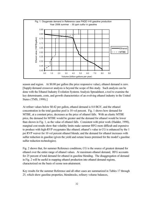
Fig. 1. <strong>Oxygenate</strong> demand <strong>in</strong> Reference case PADD I+III gasol<strong>in</strong>e production<br />
Year 2006 summer - 30 ppm sulfur <strong>in</strong> gasol<strong>in</strong>e<br />
<strong>Ethanol</strong> value (1997$/gallon)<br />
0.85<br />
0.80<br />
0.75<br />
0.70<br />
0.65<br />
0.60<br />
0.55<br />
0.50<br />
0.45<br />
0.40<br />
0.0 1.0 2.0 3.0 4.0 5.0 6.0 7.0 8.0 9.0<br />
Volume (billion gallons per year)<br />
32<br />
<strong>Ethanol</strong><br />
MTBE<br />
season and region. At $0.80 per gallon (the price responsive value), ethanol demand is zero.<br />
[Supply/demand crossover analysis is beyond the scope <strong>of</strong> this study. Such analysis can be<br />
done with the <strong>Ethanol</strong> Industry Evolution Systems Analysis Spreadsheet, a tool to exam<strong>in</strong>e the<br />
key determ<strong>in</strong>ants, costs, and growth characteristics <strong>of</strong> an evolv<strong>in</strong>g ethanol <strong>in</strong>dustry <strong>in</strong> the <strong>United</strong><br />
<strong>States</strong> (TMS, 1998).]<br />
At ref<strong>in</strong>er values below $0.42 per gallon, ethanol demand is 8.0 BGY, and the ethanol<br />
concentration <strong>in</strong> the total gasol<strong>in</strong>e pool is 10 vol percent. Fig. 1 shows how demand for<br />
MTBE, at a constant price, decreases as the price <strong>of</strong> ethanol falls. With an elastic MTBE<br />
price, the demand for MTBE would be greater and the demand for ethanol would be lower<br />
than shown <strong>in</strong> Fig. 1, as the value <strong>of</strong> ethanol falls. Consistent with prior work (Hadder, 1998),<br />
marg<strong>in</strong>al cost results show that volatility limits make summer RFG more difficult and expensive<br />
to produce with high-RVP oxygenates like ethanol; ethanol’s value <strong>in</strong> CG is enhanced by the 1<br />
psi RVP waiver for 10 vol percent ethanol blends; and the demand for ethanol <strong>in</strong>creases with<br />
sulfur reduction <strong>in</strong> gasol<strong>in</strong>e (given the yield and octane losses premised for the model’s gasol<strong>in</strong>e<br />
sulfur reduction technologies).<br />
Fig. 2 shows that, for summer Reference conditions, CG is the source <strong>of</strong> greatest demand for<br />
ethanol over the entire range <strong>of</strong> ethanol values. At maximum ethanol demand, RFG accounts<br />
for 25 percent <strong>of</strong> total demand for ethanol <strong>in</strong> gasol<strong>in</strong>e blend<strong>in</strong>g. The disaggregation <strong>of</strong> demand<br />
<strong>in</strong> Fig. 2 will be useful <strong>in</strong> mapp<strong>in</strong>g ethanol production <strong>in</strong>to ethanol demand regions,<br />
characterized on the basis <strong>of</strong> ozone non-atta<strong>in</strong>ment.<br />
Key results for the summer Reference and all other cases are summarized <strong>in</strong> Tables 17 through<br />
25, which show gasol<strong>in</strong>e properties, blendstocks, ref<strong>in</strong>ery volume balances,