Steady state erosion of critical Coulomb wedges with applications to ...

B01411 HILLEY AND STRECKER: STEADY STATE EROSION OF CRITICAL COULOMB WEDGES
of the downstream profile position (x), we relate the source
area to the upstream profile length [Hack, 1957]:
A ¼ kax h ; ð4Þ
where ka and h are constants that depend on the catchment
geometry. As h increases, larger amounts of source area are
collected for a given downstream distance than when h is
low. Therefore increases in h result in more square geometry
basins than low values of h. By combining equations (3)
and (4), we express the rate of change of the channel
elevation in terms of the downstream profile distance, x:
dz
¼ Kk
dtb
m a xhmS n : ð5Þ
[10] By assuming that wedges grow in their mechanically
critical state according to equation (1), accrete material
according to equation (2), and erode by fluvial bedrock
incision (equation (5)), Hilley et al. [2003] derive an
expression for the temporal rate of change of the basal
decollement angle as a function of the erosional and
mechanical parameters of the wedge:
db
dt ¼
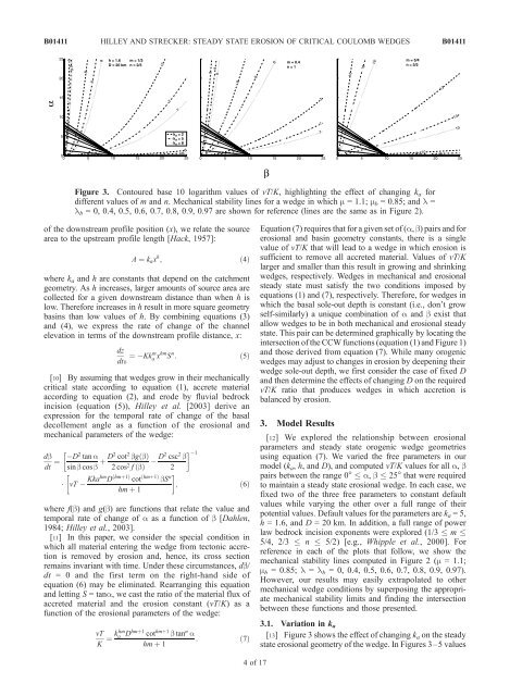
Figure 3. Contoured base 10 logarithm values of vT/K, highlighting the effect of changing k a for
different values of m and n. Mechanical stability lines for a wedge in which m = 1.1; m b = 0.85; and l =
l b = 0, 0.4, 0.5, 0.6, 0.7, 0.8, 0.9, 0.97 are shown for reference (lines are the same as in Figure 2).
D2 tan a
sin b cos b þ D2 cot2 bgðÞ b
2 cos2 f ðÞ b
D2 csc2 b
2
vT KkahmD hmþ1 ð Þcot hmþ1 ð ÞbSn hm þ 1
; ð6Þ
where f(b) and g(b) are functions that relate the value and
temporal rate of change of a as a function of b [Dahlen,
1984; Hilley et al., 2003].
[11] In this paper, we consider the special condition in
which all material entering the wedge from tectonic accretion
is removed by erosion and, hence, its cross section
remains invariant with time. Under these circumstances, db/
dt = 0 and the first term on the right-hand side of
equation (6) may be eliminated. Rearranging this equation
and letting S =tana, we cast the ratio of the material flux of
accreted material and the erosion constant (vT/K) as a
function of the erosional parameters of the wedge:
vT
K
¼ khm
a Dhmþ1 cothmþ1 b tann a
: ð7Þ
hm þ 1
1
4of17
B01411
Equation (7) requires that for a given set of (a, b) pairs and for
erosional and basin geometry constants, there is a single
value of vT/K that will lead to a wedge in which erosion is
sufficient to remove all accreted material. Values of vT/K
larger and smaller than this result in growing and shrinking
wedges, respectively. Wedges in mechanical and erosional
steady state must satisfy the two conditions imposed by
equations (1) and (7), respectively. Therefore, for wedges in
which the basal sole-out depth is constant (i.e., don’t grow
self-similarly) a unique combination of a and b exist that
allow wedges to be in both mechanical and erosional steady
state. This pair can be determined graphically by locating the
intersection of the CCW functions (equation (1) and Figure 1)
and those derived from equation (7). While many orogenic
wedges may adjust to changes in erosion by deepening their
wedge sole-out depth, we first consider the case of fixed D
and then determine the effects of changing D on the required
vT/K ratio that produces wedges in which accretion is
balanced by erosion.
3. Model Results
[12] We explored the relationship between erosional
parameters and steady state orogenic wedge geometries
using equation (7). We varied the free parameters in our
model (ka, h, and D), and computed vT/K values for all a, b
pairs between the range 0° a, b 25° that were required
to maintain a steady state erosional wedge. In each case, we
fixed two of the three free parameters to constant default
values while varying the other over a full range of their
potential values. Default values for the parameters are ka =5,
h = 1.6, and D = 20 km. In addition, a full range of power
law bedrock incision exponents were explored (1/3 m
5/4, 2/3 n 5/2) [e.g., Whipple et al., 2000]. For
reference in each of the plots that follow, we show the
mechanical stability lines computed in Figure 2 (m = 1.1;
mb = 0.85; l = lb = 0, 0.4, 0.5, 0.6, 0.7, 0.8, 0.9, 0.97).
However, our results may easily extrapolated to other
mechanical wedge conditions by superposing the appropriate
mechanical stability limits and finding the intersection
between these functions and those presented.
3.1. Variation in ka
[13] Figure 3 shows the effect of changing ka on the steady
state erosional geometry of the wedge. In Figures 3–5 values