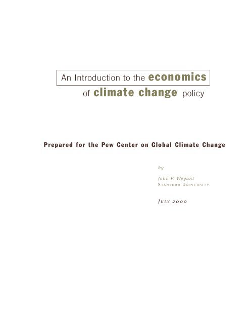
An Introduction to the economics of climate change policy

An Introduction to the e c o n o m i c s 

o f c l i m a t e change p o l i c y 

Prepared for the Pew Center on Global Climate Change 

by 

John P. Wey ant 

S TA N F O R D U N I V E R S I T Y 

J U LY 2 0 0 0

Contents 

Foreword ii 

E xecutive Summary iii 

I. Introduction 1 

II. An Economics Approach to Climate Change Policy Analysis 3 

A. Analytical Frameworks 3 

B. The Role of Energy Prices 5 

III. Five Determinants of Climate Change Cost Estimates 8 

A. Projections of Base Case Emissions and Climate Damages 8 

B. The Climate Policy Regime Considered 10 

C. Representation of Substitution Possibilities by Producers and Consumers 14 

D. Technological Change 20 

E. Characterization of Benefits 25 

I V. Information and Insights From Applications of Economic Models 30 

A. Base Case Emissions Projections 30 

B. The Climate Policy Regime Considered 32 

C. Substitution Opportunities 36 

D. Technological Change 38 

E. Benefits of Emissions Reductions 42 

V. Conclusions 44 

Endnotes 47 

References 49 

An Introduction to the economics of climate change policy 

+ 

+ 

i 

+

+ 

+ 

ii 

+ 

Foreword E il e en Claus sen , Presi d ent , Pew Cent er on Glob al Climate Chan g e 

What are the potential costs of cutting greenhouse gas emissions? Can such reductions be achieved 

without sacrificing economic growth or the standard of living we have come to enjoy? These are important ques- 

tions, and they come up again and again as the United States and other nations consider what actions are 

needed in response to climate change. 

Many participants in the climate change debate — in government, industry, academia, and non- 

g o v e rnmental organizations — have conducted economic assessments to determine the costs of taking various 

actions to address climate change, with the number of economic assessments increasing exponentially in 

recent years. Diff e rences among their quality and predicted cost of action, or inaction, have also grown, making 

it difficult to have faith in any one analysis. 

The primary example of varying model results can be seen among the numerous re p o rts predicting the 

domestic costs of complying with the Kyoto Protocol. Some have concluded the United States can reduce its 

emissions significantly below its Kyoto target (7 percent below 1990 levels), with net economic savings. Others 

have predicted dire effects on the U.S. economy. The truth most likely lies somewhere in-between. 

Behind each analysis is an economic model with its own set of assumptions, its own definitions of how 

the economy works, and its own data sets. Unfort u n a t e l y, these models often seem to be impenetrable "black 

boxes" allowing only a select few to decipher and interpret their re s u l t s . 

F o rt u n a t e l y, along with the rise in economic modeling there has also been a focus on identifying the 

d i ff e rences among models. Professor John Weyant of Stanford University, the author of this re p o rt, has been at 

the fore f ront of these eff o rts as Director of the Energy Modeling Forum of Stanford University (EMF). His EMF 

working group convenes the world’s leading energy and climate modelers to discuss and model current energ y 

policy topics. 

In this re p o rt, Professor Weyant identifies the five determinants that together explain the majority of 

d i ff e rences in modeling cost estimates. This is great news for those engaged in the climate change policy are n a 

who are consumers of economic modeling results. Five key questions can be raised to help policy-makers 

understand the projected costs of climate change policy: What level of greenhouse gas emissions are pro j e c t e d 

under current policies? What climate policies are assumed to be put in place to achieve emissions re d u c t i o n s ? 

What assumptions are made about how advances in technology might affect these emissions? To what extent 

a re environmental impacts of climate change included? And is the full set of choices that firms and consumers 

have when presented with rising energy prices accounted for? 

This paper would not have been possible without the assistance of numerous individuals. The author 

and the Pew Center would like to thank Ev Ehrlich, Judi Greenwald, Larry Goulder, Henry Jacoby, Rich Richels, 

Dick Goettle, Bill Nordhaus, and Bob Shackelton for their thoughtful comments on previous drafts of this paper. 

We acknowledge the use of material from a background paper pre p a red by Robert Repetto, Duncan 

Austin and Gwen Parker at World Resources Institute. 

An Introduction to the e c o n o m i c s of climate change policy

E xecutive Summary 

This paper is an introduction to the economics of climate change policy. The goal is to help the 

reader understand how analysts use computer models to make projections of mitigation costs and climate 

change impacts, and why projections made by diff e rent groups diff e r. In order to accomplish this goal, 

the paper will describe five key determinants of greenhouse gas (GHG) mitigation cost estimates. 

The paper starts with a discussion of how the economy would adjust to restrictions on GHG 

emissions, especially carbon dioxide, the dominant, and easiest to measure GHG produced in the United 

States. Combustion of fossil fuels — oil, gas, and coal — produces large amounts of carbon dioxide. 

Central to this discussion is the role of energy price increases in providing the incentives for corporations 

and individuals to reduce their consumption of these fuels. 

E n e rgy price increases cause producers to substitute among the inputs they use to make goods 

and services, and consumers to substitute among the products they buy. Simultaneously, these price 

i n c reases provide incentives for the development of new technologies that consume less energy in pro v i d- 

ing the goods and services that people desire. How a model re p resents these substitution and innovation 

responses of the economy are important determinants of the economic impacts of restrictions on GHGs. 

T h ree other factors are crucial to economic impact projections. 

First, the projected level of baseline GHG emissions (i.e., without any control policies) 

d e t e rmines the amount of emissions that must be reduced in order to achieve a particular emissions 

t a rget. Thus, other things being equal, the higher the level of base case emissions, the greater the 

economic impacts of achieving a specific emissions target. The level of base case emissions depends, in 

t u rn, on how population, economic output, the availability of energy fuels, and technologies are expected 

to evolve over time without climate change policies. 

The second factor is the policy regime considered, i.e., the rules that govern the possible 

adjustments that the economy might make. International or domestic trading of GHG emissions rights, 

An Introduction to the e c o n o m i c s of climate change policy 

+ 

+ 

iii 

+

+ 

+ 

+ 

i n t e r-gas trading among all GHGs, inclusion of tree planting and carbon sequestration as mitigation 

options, and complementary economic policies (e.g., using carbon tax revenues to reduce the most 

d i s t o rt i o n a ry taxes in the economy) are all elements of the policy regime. Other things being equal, the 

m o re flexibility provided in the policy regime under consideration, the smaller the economic impacts of 

achieving a particular emissions target. 

The third factor is whether the benefits of reducing GHG emissions are explicitly considered. An 

analyst may subtract such benefits from the mitigation cost projection to get a “net” cost figure or pro- 

duce a “gross” cost figure that policy-makers can weigh against a benefit estimate. The kind of cost fig- 

u re produced often depends on whether the analyst is trying to do a cost-benefit analysis or an analysis 

focused on minimizing the cost of reaching a particular emissions target. 

Thus, this paper will describe the major input assumptions and model features to look for in 

i n t e r p reting and comparing the available model-based projections of the costs and benefits of GHG 

reductions. Two of the five key determinants — (1) substitution, and (2) innovation — are stru c t u r a l 

f e a t u res of the economic models used to make emissions projections. The other three determinants are 

e x t e rnal factors, or assumptions. They are: (3) the base case projections, (4) the policy regime consid- 

e red, and (5) the extent to which emissions reduction benefits are considered. 

The results summarized in this paper illustrate the importance of these five determinants and the 

l a rge role played by the external factors or assumptions. Cost projections for a given set of assumptions 

can vary by a factor of two or four across models because of diff e rences in the models’ re p resentation of 

substitution and innovation processes. However, for an individual model, diff e rences in assumptions 

about the baseline, policy regime, and emissions reduction benefits can easily lead to a factor of ten or 

m o re diff e rence in the cost estimates. Together these five determinants explain the majority of diff e re n c e s 

in economic modeling results of climate policy. 

iv An Introduction to the e c o n o m i c s of climate change policy

I. Introduction 

Int erest groups active in the cl i m ate change deb ate bel i eve that the 

st akes are hi gh . Some fear the environmental and socioeconomic costs of climate change itself. 

Others are more fearful of the economic consequences of trying to avoid climate change. 

This debate is, to a large extent, played out through economic analysis of climate change policy. 

H u n d reds of these analyses have been published over the past decade, and this pace is likely to 

continue. Several federal agencies perf o rm in-house analyses or fund independent re s e a rch to determ i n e 

the costs of various policy options. Interest groups on all sides of the debate do the same. These analyses 

a re rich and extensive, but widely divergent in their results. 

T h rough these economic analyses, people translate their expectations into concrete assumptions 

about the future. The set of assumptions that describe what happens in the future if nothing is done to 

c o n t rol greenhouse gas (GHG) emissions is known as the “base case” (or as the “baseline” or “business- 

as-usual” case). The base case may embody optimism or pessimism about GHG emissions, about the 

changes in climate that will occur as a result of these emissions, and about what will happen to the 

e n v i ronment as a result of this climate change. 

The base case also may embody optimism or pessimism about what will happen to the economy. 

The higher the base case emissions, the more emissions must be reduced to achieve a particular targ e t , 

and there f o re the higher the control costs. The greater the base case climate impacts, the greater the 

benefits of controlling emissions. 

Another set of assumptions drives projections of what will happen if society does control GHGs. 

Will new, low-cost, low-emitting technologies become available? Will consumers and producers re s p o n d 

c l e v e r l y, meeting their needs diff e rently but equally well through lower-emitting products and serv i c e s ? 

Economic analyses may embody optimism or pessimism on either of these fro n t s . 

A third set of assumptions is related to how society goes about requiring GHG control, i.e., what 

policies the government will put in place. Will the policies be flexible, allowing targets to be met at 

significantly lower costs? For example, one key aspect of the policy regime is the extent to which 


+ 

+ 

1 

+

+ 

+ 

+ 

emissions trading is allowed. Another key aspect is the inclusiveness of the policy. Will carbon-absorbing 

activities, such as tree-planting, count as an offset to carbon emissions? Will all GHG emissions count, 

and will inter-gas trading be perm i t t e d ? 

F i n a l l y, most quantitative analyses only address the control costs, and not the environmental ben- 

efits, of reducing GHGs. Cost-benefit analyses may show either net benefits or net costs of GHG contro l s , 

depending, to a large extent, on the range of environmental benefits that are included in the analyses. 

The tools people employ to perf o rm these complex economic analyses are large computer models. 

Model results vary widely due mainly to diff e rences in the above assumptions. For example, among the 

14 models and dozens of model runs reviewed for this paper, the base case forecasts range from a 20 

p e rcent to a 75 percent increase in carbon emissions by 2010. 

One rough measure of economic costs is the carbon price—the amount of money one would have 

to pay to reduce emissions by a ton of carbon. Among the model results reviewed here, carbon price 

f o recasts for meeting the U.S. emissions targets of the Kyoto Protocol ranged from less than $20 per ton 

to over $400 per ton. This variation may result from using diff e rent models, as well as from using the 

same model with diff e rent input assumptions. 

The economic consulting firm Wharton Econometric Forecasting Associates (WEFA) issued a 

re p o rt in 1998 projecting a carbon price of $360 per ton associated with U.S. GHG reductions. WEFA is 

pessimistic about both the development of new technologies and the ability of businesses to think ahead 

and begin responding early. WEFA also assumes relatively inflexible government policies — i.e., it 

assumes that it will not be possible to reduce GHGs other than carbon dioxide(CO2), employ carbon sinks, 

or engage in international emissions trading by the time of the first Kyoto budget period (2008-2012). In 

contrast, the Pre s i d e n t ’s Council on Economic Advisors published an “official” analysis in 1998 in which 

the carbon price under Kyoto would be quite low — on the order of $20 per ton — largely because it 

assumed that the United States would purchase most of its emissions reductions overseas through inter- 

national emissions trading. 

In many cases the assumptions that drive economic models are readily apparent; in other cases 

they are difficult to tease out because they are embedded in detailed aspects of the model’s stru c t u re . 

The goal of this paper is to demystify what is driving these model results, thereby enabling the reader to 

p a rticipate fully in one of the most important debates of our time. 

2 


II. An Economics Approach to Climate Change Policy Analysis 

Ec on omic an alysis is a rigorous appro a ch to ev alu ating the costs an d 

b enef i ts of al t er n at ive pol i c i es. D i ff e rent economic analysts use diff e rent “analytical frame- 

works” — i.e., they differ as to how they measure costs, what impacts they consider, and how they handle 

u n c e rt a i n t y. In dealing with climate change, economists are particularly interested in how energy price 

i n c reases cause corporations and individuals to reduce their consumption of carbon-based fuels. The goal 

of this section is to help the reader understand how economists approach climate change policy analysis. 

A. Analytical Frameworks 

A cl i m ate pol i cy an alysis of t en pro c e e ds in a line ar manner. It begins with 

the initial projection of GHG emissions to the atmosphere, followed by several calculations based on 

climate change science, and eventually ends with a projection of the resulting climate change impacts 

f rom those emissions. Thus, one could simply calculate the climate change impacts resulting from a 

p a rticular emissions trajectory. Altern a t i v e l y, one could work backwards from an acceptable set of climate 

impacts to find the emissions trajectories that are consistent with those impacts. One could also set a 

t a rget for the maximum level of GHG emissions, concentration level of GHGs in the atmosphere, magni- 

tude of climate change, or extent of climate impacts and compute the least-cost way to achieve that 

objective. This formulation is re f e rred to as cost-effectiveness analysis and, if there is a range of “accept- 

able impacts,” as the “tolerable windows” approach. 

If one can estimate the value of all the climate change impacts in a common unit of 

m e a s u rement, one can add them together. Then the net benefits (i.e., the benefits of reduced climate 

change impacts, minus the costs of climate change mitigation) of an emissions reduction policy can be 

calculated. This approach is re f e rred to as cost-benefit analysis. The result of a cost-benefit analysis is 

the optimal GHG “price” and the corresponding level of emissions reduction. The studies looking at 

impacts differ in three ways: (1) the cost measure employed, (2) the range of climate change impacts 

c o n s i d e red, and (3) how uncertainty is handled. 


+ 

+ 

3 

+

+ 

+ 

+ 

Cost Measure 

T h e re are numerous methods for measuring the economic costs and/or benefits employed in 

economic models. These methods can range from total re s o u rce costs, 1 to measures of aggregate econom- 

ic output like Gross National Product, to rough measures of economic welfare like the discounted pre s e n t 

value of consumption, 2 to more precise measures of economic welfare like “compensating variation.” 

Compensating variation measures the amount of additional income that would have to be provided to 

consumers to make them as well off after a policy is implemented as they were before the policy’s 

imposition. The selection of the cost measure to be optimized depends on the stru c t u re of the model and 

on the interests and objectives of the model users. For example, a model that does not include a utility 

f u n c t i o n 3 in its objective cannot produce the discounted utility of consumption or compensating variation 

m e a s u res. On the other hand, someone who is particularly interested in the magnitude of the impact on 

the energy sector may use a model with a great deal of energy sector detail and use the change in total 

re s o u rce costs as a measure of that impact. 

Range of Impacts Considere d 

Sometimes the costs of climate change impacts and the reductions in those impacts that are 

attributable to emissions reduction policies are considered in economic models, and sometimes they are 

not. Also, diff e rent studies may consider diff e rent impacts. (See Section III.E for more description of 

these impacts). 

U n c e rtainty 

T h e re are considerable uncertainties about mitigation costs, and even greater uncertainties about 

climate change impacts. There is uncertainty about societal values and uncertainty about model 

s t ru c t u re. It is important to understand how a given analytical framework treats these uncertainties. 

To many analysts, the best way to formulate the problem of climate change is as a problem of 

sequential decision-making under uncert a i n t y. These methods are still in their infancy and lacking 

i m p o rtant data necessary for analysis, such as data on alternative policies, pre f e rences of stakeholders 

(e.g., developing country citizens), and probabilities of various outcomes (Kann and Weyant, 2000). This 

re p o rt ’s focus is on U.S. cost and benefit estimates. 

4 An Introduction to the e c o n o m i c s of climate change policy

B. The Role of Energy Prices 

T he price of energy is very imp or t ant in cl i m ate change econ om i c 

m o d el s. Most economic models solve a set of mathematical equations to obtain the prices of goods 

and services. The simultaneous solution of these equations re p resents an equilibrium in which supply 

equals demand among consumers and producers. In this framework, an energy price increase can be 

either the motivation for, or the result of, GHG emissions reductions. For example, governments may 

impose emissions taxes to motivate GHG reductions. Emissions taxes raise the costs of fuels dire c t l y, and 

economies will adjust to reduce the use of those higher-cost fuels, substituting goods and services that 

result in fewer GHG emissions. On the other hand, governments may cap the total amount of emissions, 

distribute or sell emissions “allowances,” and let the market determine the price and distribution of these 

allowances. Such a “cap and trade” system will induce changes in prices that are difficult to pre d i c t . 

Since a cap would essentially restrict the supply of carbon-based fuels, GHG consumers would bid up the 

price until demand for such fuels no longer exceeded supply. In this way the higher prices re d u c e 

emissions, but also allocate the GHGs to their highest-value uses. 

The effects of higher fossil fuel prices would diffuse throughout the economy. Prices of secondary 

e n e rgy sources, like electricity and oil products, would rise as the higher primary fuel costs are passed 

t h rough into electricity rates, fuel oil, and gasoline prices. Higher fuel costs would also increase operating 

costs in transportation, agriculture, and especially industry. Although energy costs make up only 

2.2 percent of the total costs in U.S. industry, they constitute up to 25 percent of the total costs in the 

most energy-intensive sectors (e.g., iron and steel, aluminum, paper-making, and chemicals). Each indus- 

t ry ’s ability to pass these cost increases along to customers through higher product prices would depend 

on the strength of the demand for its products, and on the severity of international competition. Since 

many of the major trading partners of the United States would also be implementing similar climate poli- 

cies, it is likely that the energy cost increase would result in higher prices for a broad range of consumer 

p roducts. Households could also be affected through increased heating, transportation, and utility bills 

and, to a lesser degree, food bills and other costs of living. 

A host of adjustments by producers and consumers in the economy would take place in parallel 

with the price increases, and, in fact, these substitutions would also serve to limit the extent of the price 

i n c reases that would ultimately result. Higher energy costs would induce firms to accelerate the 


+ 

+ 

5 

+

+ 

+ 

+ 

replacement of coal-based or obsolete plants with more energ y - e fficient or less carbon-intensive 

equipment. Utilities and their customers would seek alternatives to carbon-intensive coal-fired power 

plants, stimulating the market for hydro - p o w e red, nuclear, gas-fired, and renewable electricity. As coal 

prices rise relative to natural gas prices, modern gas-fired combined cycle power plants would become 

even more competitive. Older, less-efficient coal-fired plants would probably be re t i red from service, or 

re s e rved for intermittent operations. Energy-intensive industries would also face a number of adjustment 

decisions: whether to re t i re obsolete facilities and concentrate production at more modern, low-cost 

facilities; whether to modify their furnaces to burn gas instead of coal; whether to generate their own 

electricity; whether to invest in a wide variety of energ y - c o n s e rving process changes; whether to re d e s i g n 

p roducts to save energy; and whether to alter their product mix. Ultimately, there would be an eff e c t i v e 

diminution in the value of the existing stock of plant and equipment because the existing capital stock is 

optimized for the set of input prices that prevailed when it was installed and would be sub-optimal for the 

new price re g i m e . 

In the short run, consumers and producers would reduce their energy consumption by either 

consuming fewer energy services (for example, turning their thermostats down or driving their automobiles 

less), or producing less output. Consumers and producers may also, potentially, reduce energy use without 

reducing output by identifying energy efficiency measures previously believed not to be economical. 

In the intermediate time frame, there might be opportunities for fuel switching (or substitutions 

between other inputs) that would not involve substantial outlays for new equipment or infrastru c t u re (for 

example, switching the fuel used in a multi-fuel-capable boiler from oil or coal to gas). In addition, 

consumers may be able to substitute goods that re q u i re less energy to produce (which would become 

relatively less expensive) for more energy-intensive ones (which would become relatively more expensive). 

In the long term, new technologies would be purchased that either use less GHG-intensive fuel or 

a re more fuel-efficient. In addition, new, less GHG-intensive technologies might become available over 

time as a result of re s e a rch and development (R&D) expenditures or cumulative experience. The 

e m e rgence of these new technologies might be related to the energy price increases, the base case tre n d 

of all other prices, or simply the passage of time. Higher energy prices would lead to less energy use, and 

less energy use would decrease the productivity of capital and labor. These productivity changes would, in 

t u rn, generally result in a slowdown in the accumulation of capital equipment and infrastru c t u re, and in 


lower wages for workers. Ultimately, even after all the adjustments have been made, consumers would 

have somewhat less income. This might cause them to adjust the amount of time they spend on work 

rather than leisure . 4 This last adjustment would involve an additional change in welfare. Offsetting these 

w e l f a re losses would be the benefits of reduced climate change, and the benefit of making those re s p o n- 

sible for GHG emissions pay for the damages they cause. 

The complicated web of economic adjustments that would take place in response to rising 

prices of energ y, or energy scarc i t y, makes the task of projecting the costs of GHG mitigation a 

challenge. Interpreting the results diff e rent models produce is further complicated because diff e re n t 

modeling systems emphasize diff e rent dimensions of the adjustment process. Also, diff e rent 

policy-makers may be interested in diff e rent policy regimes, and in diff e rent impacts of climate change 

and climate change policies. 


+ 

+ 

7 

+

+ 

+ 

8 

+ 

III. Five Determinants of Climate Change Cost Estimates 

F ive major det er m i n ants of GHG mitigat i on cost and benefit proj e c t i ons 

are disc us sed in this pap er. Understanding how diff e rent forecasters deal with these determ i- 

nants can go a long way toward understanding how individual estimates differ from one another. The five 

major determinants considered in this chapter are: 

• projections for base case GHG emissions and climate damages; 

• the climate policy regime considered (especially the degree of flexibility allowed in meeting the 

emissions constraints); 

• the re p resentation of substitution possibilities by producers and consumers, including how the 

t u rnover of capital equipment is handled; 

• how the rate and processes of technological change are incorporated in the analysis; and 

• the characterization of the benefits of GHG emissions reductions in the study, including especially 

how and what benefits are included. 

A. Projections of Base Case Emissions and Climate Damages 

Projecting the costs as so c i ated with re ducing GHG em is si ons st ar ts 

w i th a proj e c t i on of GHG em is si ons over time, as suming no new cl i m at e 

p ol i c i es. This “base case” is often an important and under- a p p reciated determinant of the re s u l t s . 

The higher the base case emissions projection, the more GHG emissions must be reduced to achieve 

a specified emissions target. If a base case is higher, though, there may be more opportunities for 

cheap GHG mitigation due to a slow rate of technological pro g ress assumed in the base case. 

The base case emissions 5 and climate impact scenarios, against which the costs and benefits 

of GHG mitigation policies are assessed, are largely the product of assumptions that are external to 

the analysis. 


Each GHG mitigation cost analysis relies on input assumptions in three areas: 

• population and economic activity; 

• energy re s o u rce availability and prices; and 

• technology availability and costs. 

Most of the re s e a rchers projecting the cost of reducing carbon emissions have relied on 

worldwide population growth projections made by others (e.g., the World Bank or the United Nations). 

These external projections are generally based on results from very simple demographic models. There is 

less uncertainty about projections for the developed countries, where population is expected to peak very 

soon, than for the developing countries, where population is typically assumed to peak somewhere aro u n d 

the middle of this century. Ve ry few of the re s e a rchers analyzing GHG emissions reductions make their 

own projections of economic gro w t h . 6 Most rely on economic growth projections made by others, or on 

e x t e rnal assumptions about labor force participation and productivity growth. 

Another set of key assumptions concerns the price and/or availability of energy re s o u rces. The 

prices of fossil fuels — oil, natural gas, and coal — are important because producers and consumers 

generally need to substitute away from these fuels when carbon emissions are restricted. Optimistic 

assumptions about natural gas availability and/or substitutability 7 can make carbon emissions re d u c t i o n s 

easier to achieve in the short run. This is because carbon emissions from natural gas per unit of energ y 

consumed are about 60 percent of those from coal, and 80 percent of those from oil. In addition, the 

amount of unconventional oil and gas production that will ultimately be technically and economically 

feasible is highly uncertain. It depends on future economic incentives for oil and gas exploration and 

p roduction, which could (absent climate policies) re t a rd the development of carbon-free renewable and 

h i g h e r- e fficiency end-use energy technologies. How oil exporters would react to a climate policy that 

would reduce the demand for oil imports is another key dimension of the energy supply picture. 

Other key assumptions are made about the costs and efficiencies of current and future energ y - 

supply and energy-using technologies. These tend to be critical determinants of energy use in both the 

base case and control scenarios. Most analysts use a combination of statistical analysis of historical data 

on the demand for individual fuels, and process analysis of individual technologies in use or under devel- 

opment, in order to re p resent trends in energy technologies. Particularly important, but difficult, is 


+ 

+ 

9 

+

+ 

+ 

+ 

p rojecting technological pro g ress within the energy sector itself. Attempts to systematically and 

empirically estimate future trends in energy productivity at a national level are rare (see Jorgenson and 

Wilcoxen, 1991, for one prominent example). Ty p i c a l l y, analysts take one of the following two appro a c h e s 

or a hybrid of the two: (1) the costs and efficiencies of energy-using and energ y - p roducing technologies 

a re projected based on process analysis, and the characteristics of these technologies are extrapolated 

into the future, or (2) some assumption is made about the trend in energy demand per unit of economic 

a c t i v i t y, independent of future price increases. (See Section III. D on technological change for a more 

detailed description). Some recent analyses have attempted to blend the two approaches. At some point 

these two approaches tend to converge, as the end-use process analyst usually runs out of new 

technologies to predict. It is then assumed that the efficiency of the most efficient technologies for which 

t h e re is an actual proposed design will continue to improve as time goes on. 

P rojections of the benefits of reductions in GHG emissions are also highly dependent on the base 

case scenario employed. The greater the base case damages (i.e., the damages that would occur in the 

absence of any new climate policies), the greater the benefits of a specific emissions target. The 

magnitude of the benefits from emissions reductions depends not only on the base case level of impacts 

but also on where they occur, and on what sectors are being considered. In fact, a number of additional 

socio-economic inputs (e.g., income by economic class and region, infrastru c t u re, and institutional 

capability to adapt to changes, etc.) are re q u i red because they determine how well the aff e c t e d 

populations can cope with any changes that occur. The task of projecting base case climate change 

impacts is particularly challenging because: (1) most assessments project that serious impacts re s u l t i n g 

f rom climate change will not begin for several decades, and (2) most of the impacts are projected to 

occur in developing countries where future conditions are highly uncertain. How well developing countries 

can cope with future climate change will depend largely on their rate of economic development. 

B. The Climate Policy Regime Considered 

T he pol i cy re gi me consi d ered is a cruc i al source of differen c es in cost 

and benefit proj e c t i ons and is larg ely indep en d ent of the model meth o dol o gy 

use d . Once a base case scenario is constructed, the types of policies that nations may use to satisfy 

their GHG emissions obligations must be specified. 


The Kyoto Protocol re p resents a broad approach to undertaking emissions reductions. This 

a p p roach tentatively includes flexibility in determining which GHGs can be reduced, where they can be 

reduced, and, to a lesser extent, when they can be reduced. These flexibility mechanisms are explicitly 

mentioned in the Kyoto Protocol. However, the flexibility mechanisms are: 

• already explicitly limited (as in the five-year emissions averaging period — rather than a 

longer one); 

• potentially subject to restrictions as a result of further negotiations (like those being contemplated 

on international emissions rights trading under the Kyoto Protocol); or 

• potentially difficult to implement because of measurement, monitoring, and data limitations (as in 

the case of non-carbon dioxide GHG emissions and carbon sinks). 

Thus, there are large uncertainties about the extent to which the Kyoto flexibility mechanisms 

can be employed, and there f o re about their value. If the parties to the Protocol can avoid restricting these 

mechanisms, and can surmount definitional and other obstacles to their implementation, the flexibility 

mechanisms can reduce the price increases (and associated impacts) re q u i red to achieve the objectives 

of the Protocol by a factor of ten or more. 

An important flexibility mechanism in the Kyoto Protocol is that nations have agreed to consider 

six principal GHGs: CO 2, methane (CH 4), nitrous oxide (N 2O), sulfur hexaflouride (SF 6), perf l u o u ro c a r b o n s 

(PFCs), and hydro f l u o rocarbons (HFCs), and to allow inter-gas trading. 8 These GHGs differ both in their 

heat-trapping capacity and in the length of time they remain in the atmosphere. CO 2 is the most 

significant contributor to global climate change among global GHG emissions. The Protocol also specifies 

that taking CO 2 out of the atmosphere (i.e., through carbon “sinks”) can count towards each country ’s 

emissions reduction commitment. 9 

Another flexibility mechanism included in the Kyoto Protocol is international emissions trading. 

T h e re are benefits from international emissions trading because there are diff e rences in the costs of 

reducing emissions among countries. 1 0 If the cost of emissions reductions in any country is higher than it 

is in any other country, it is advantageous to both countries for the higher cost country to buy emissions 

“rights” from the lower cost country at a price that is between the two cost levels. 1 1 If one aggregates all 

regions participating in the trading system together, one can compute the supply and demand for 


+ 

+ 

11 

+

+ 

+ 

+ 

emissions rights at any price, as well as the equilibrium emissions rights price that balances the available 

supply with the amount demanded. 

The Protocol also allows participants to average emissions over a five-year period (2008-2012, 

also known as the first budget period) in satisfying their emissions reduction re q u i rements. Av e r a g i n g 

allows corporations and households to shift their reductions in time to reduce the economic impact of the 

re q u i red emissions reductions. A number of studies indicate that this emissions averaging can be helpful 

in cutting the cost of reducing cumulative emissions but that an even longer averaging period would be 

1 2 

m o re advantageous. 

Revenue Recycling 

An important issue in climate-policy discussions has been the extent to which the costs of 

carbon taxes (or carbon permit auctions) can be reduced by judicious “recycling” of the revenues fro m 

such taxes — i.e., using the carbon tax revenues to justify, and to offset, decreases in other taxes. This is 

primarily a domestic policy flexibility mechanism, although the international negotiations at some point 

may address how carbon tax revenues can be recycled. Economists’ understanding of this issue has 

advanced considerably in recent years. Theoretical work indicates that the costs of carbon taxes can be 

significantly reduced by using the revenues to finance cuts in the marginal rates of existing income taxes, 

as compared with re t u rning the revenues to the economy in a “lump-sum” fashion. Lump-sum distribu- 

tions are those in which the transfers are independent of taxpayer behavior (for example, the personal 

exemptions in income taxes are lump-sum transfers). Numerical studies consistently confirm this re s u l t 

(see Shackleton, 1996; Goulder, 1995; Jorgenson and Wilcoxen, 1995). 

A more controversial issue has been whether revenue recycling can make the gross costs of 

revenue-neutral carbon tax policies vanish or become negative. If this were the case, the re v e n u e - n e u t r a l 

e n v i ronmental tax would generate a “double dividend” by both: (1) improving the environment, and 

(2) reducing the costs of the tax system. Recent theoretical work on this issue tends to cast doubt on the 

likelihood of a double dividend (Bovenberg and de Mooij, 1994; Parry, 1995; Bovenberg and Goulder, 

1997). This work indicates that carbon taxes may be less efficient sources of revenue than the income 

taxes they would replace. The key to this result is the recognition that carbon taxes (like other taxes) cause 

output prices to rise, and thereby lower the real re t u rns to primary inputs into production like labor and 


capital. As a result, carbon taxes cause market distortions that are quite similar to those posed by income 

taxes. Carbon taxes also have an efficiency disadvantage attributable to their relatively narrow base. 

Still, economic theory leaves room for the double dividend under some special circ u m s t a n c e s . 

In part i c u l a r, it can arise if: (1) the original tax system (prior to introducing the carbon tax) is seriously 

i n e fficient along some non-environmental dimension (e.g., capital might be highly overtaxed relative to 

labor), and (2) the revenue-neutral re f o rm reduces this inefficiency enough to offset the carbon tax’s 

e fficiency disadvantage. Whether or not the double dividend would arise thus depends on some 

empirical issues. Analyses with numerical general equilibrium models 1 3 tend to cast doubt on the 

p rospects for the double dividend in the United States (Bovenberg and Goulder, 1997). However, the 

p rospects could be better in other countries, especially in economies with subsidized energ y. Removing 

e n e rgy subsidies is likely to lower the costs of the tax system while promoting an improvement in the 

e n v i ronment. Energy is subsidized in a number of developing countries, and thus the costs of re d u c i n g 

carbon emissions may be minimal or negative in these countries. Further empirical investigations of this 

issue could be valuable to policy-makers. 

A practical difficulty in studying revenue recycling is what assumptions about recycling are most 

realistic. Since tax systems are continually debated and revised, it is not clear whether the most 

i n e fficient taxes would be eliminated at some point, independent of the availability of carbon tax re v- 

enues to offset them as a source of revenue. There is also a political economy challenge to using re v e n u e 

recycling as part of a carbon emissions reduction strategy. Rather than using the new tax revenues to 

reduce other more distort i o n a ry taxes, society could easily use them to support additional govern m e n t 

spending. Such government outlays could have lower or higher productivity than the same amount of 

private sector spending (see Nordhaus, 1993). If the government expenditure has lower pro d u c t i v i t y, the 

overall costs of the carbon tax would be considerably higher than when revenues are employed to finance 

cuts in distort i o n a ry taxes. Thus, to fully analyze the impact of revenue recycling alternatives on the 

overall cost of carbon taxation, one needs not only to analyze the impact of a carbon tax, but also to 

speculate about how the government would employ the revenues from the tax. 

I n t e rnational emissions trading, inclusion of GHGs other than CO 2, credit for carbon sinks such 

as planting trees, and judicious revenue recycling can all help reduce the costs of GHG mitigation 

policies. Any of these approaches can reduce the necessary rise in energy prices and the associated 


+ 

+ 

13 

+

+ 

+ 

+ 

impacts on economic activity. The resulting costs will depend on how easy it is for businesses and 

households to change their mix of inputs, and for consumers to change their mix of purchases, in ways 

that reduce GHG emissions. 

C. Representation of Substitution Possibilities by Producers and Consumers 

As effor ts are made to re duce GHG em is si ons , fos sil fuel combust i on 

and other GHG-generating activ i t i es become more exp ensive. P roducers adjust to 

these price increases by substituting inputs (i.e., switching to inputs that generate fewer GHG emissions 

in manufacturing any particular product), and by changing their product mix (i.e., producing diff e re n t 

p roducts that re q u i re fewer GHG emissions to make). 

The extent to which inputs can be shifted depends on the availability and cost of appro p r i a t e 

technologies as well as the turnover rate of capital equipment and infrastru c t u re. These two factors, as 

well as consumer pre f e rences, determine an industry ’s ability to produce and sell alternative mixes of 

p roducts. Increases in the costs both of fossil fuels and of products that depend on fossil fuel 

combustion will reduce consumers’ real incomes. Consumers will simultaneously decide: (1) the extent to 

which they wish to adjust their mix of purchases towards less carbon-intensive products, and (2) how to 

adjust their mix of work and leisure time to compensate for the reduction in their real income. 

S h o rt - t e rm vs. Long-term Substitution 

If businesses and households have several decades to complete the substitution process, the 

c u rrent stock of energy equipment and associated infrastru c t u re does not constrain the substitutions that 

they may make. Businesses and households are limited primarily by the available technologies, and by 

their own pre f e rences re g a rding how much of each available product they would buy at the pre v a i l i n g 

prices. If climate policy is long-term, and if economic incentives are designed to motivate producers and 

consumers to invest in more energ y - e fficient and less carbon-intensive equipment when their existing 

equipment has reached the end of its useful life, the transition to a lower carbon energy system will be 

relatively smooth and the costs relatively moderate. Over shorter time spans, however, existing plant and 

equipment can significantly constrain the behavior of firms and households, adding transition costs to the 

l o n g - run costs of GHG control policies. Policies implemented on this time scale (i.e., within ten years) 

will lead to reductions in energy services (e.g., industrial process heat and home heating and cooling), 


some easy fuel switching, and an increase in the purchase and use of available energ y - e fficient pro d u c t s 

and services. They will also influence the rate of re t i rement and replacement of existing equipment. 

E n e rg y - p roducing and energy-using equipment is relatively expensive and long-lived. Thus, it will 

generally take a substantial increase in energy prices to induce those who own such equipment to re p l a c e 

1 4 

it before the end of its useful life. 

The importance of capital stock dynamics creates a formidable challenge for the analytical 

c o m m u n i t y. Some data on the characteristics of the energ y - p roducing and energy-using capital stock are 

available. It would be ideal to have information on the costs of operating and maintaining every piece of 

equipment currently in use. This would enable analysts to calculate all the trade-offs between re t i r i n g 

equipment early and using other strategies to achieve the specified targets. Unfort u n a t e l y, the data that 

a re available are generally aggregated across large classes of consumers and generally include all existing 

capacity without re g a rd to when it was installed. An important exception is power plant data, which are 

v e ry disaggregated and include the age of the equipment. However, even these data are generally not suf- 

ficient to ascertain precisely the point at which the carbon price incentives will influence the rate of 

replacement of plant and equipment. Limitations on data re q u i re the analyst to make a number of 

assumptions re g a rding the aggregation and interpretation of the available data. 

Two Approaches to Representing Substitution Possibilities 

In many models, technologies are re p resented with “production functions” that specify what 

combinations of inputs are needed to produce particular outputs. The production function specifies the rate 

at which each input can be substituted for each other input in response to shifts in input prices. As new 

capital investment occurs and older capital is re t i red, the technology mix within the model will change. 

Two basic types of production functions may be specified: 

• aggregate production functions; and 

• technology-by-technology production functions, also known as “process analysis.” 

Some models (e.g., G-Cubed, SGM, and EPPA — see Box 1 for model identification) use smooth 

and continuous aggregate production functions that allow incremental input substitutions as prices 

change, even if the resulting input configuration does not correspond to a known technology. These 


+ 

+ 

15 

+

+ 

+ 

16 

+ 

models do not re p resent individual technologies. Such models often assume “nested” production func- 

tions. For example, at one level, substitutions are possible between energ y, capital, and labor in 

p roducing final commodities; at a second level, substitutions are possible between electricity and fuel oil 

in producing energy; and, at a third level, substitutions are possible between coal and natural gas in 

p roducing electricity. Models employing continuous aggregate production functions do not account for 

individual technologies. 

Box 1 

M O D E L A U T H O R S 

A B A R E - G T E M B. Fisher, V. Tulpule, D. Kennedy, S. Brown (ABARE) 

(Australian Bureau of Agriculture and Resourc e s 

Economics — Global Trade and Environment Model) 

A I M T. Morita, M. Kainuma (NIES, Japan) 

(Asian-Pacific Integrated Model) Y. Matsuoka (Kyoto University) 

C E TA S. Peck (EPRI) 

(Carbon Emissions Tr a j e c t o ry Assessment) T. Te i s b e rg (Te i s b e rg Assoc.) 

G - C u b e d W. McKibben (Australian National University) 

(Global General Equilibrium Growth Model) P. Wilcoxen (University of Texas), R. Shackleton (U.S. OMB) 

I G E M D. Jorgenson (Harv a rd University) 

( I n t e rtemporal General Equilibrium Model) P. Wilcoxen (University of Te x a s ) 

R. Goettle, M. Sing Ho, D. Slesnick (Dale W. Jorgenson Associates) 

M A R K A L - M a c ro S. Morris (Brookhaven National Laboratory ) 

A. Manne (Stanford University), P. Tseng (U.S. DOE) 

MERGE 3 A. Manne (Stanford University) 

(Model for Evaluating Regional and Global Eff e c t s R. Richels (EPRI) 

of GHG Reductions Policies) 

M I T- E P PA H. Jacoby, J. Reiner, I.S. Wing (MIT) 

(Emissions Projection and Policy Analysis Model) 

M S - M RT D. Montgomery, P. Bernstein (Charles River Associates) 

(Multi-Sector—Multi-Region Trade Model) T. Rutherf o rd (U. Colorado) 

N E M S R. Earley, S. Holte, M. Hutzler, A. Kydes, R. Eynon, et. al. 

(National Energy Modeling System) (U.S. Energy Information Agency) 

O x f o rd Model A. Cooper, J. Walker (Oxford Econometrics) 

( O x f o rd Econometrics Model) 

R I C E W. Nordhaus, J. Boyer (Yale University) 

(Regional Integrated Climate and Economy Model) 

S G M J. Edmonds, H. Pitcher, R. Sands (Pacific Northwest National Lab) 

(Second Generation Model) 

A Guide to Economic Models of Climate Change 

Wo r l d s c a n A. Gielen, H. Timmer (Central Planning Bureau, Netherlands) 

(Central Planning Bure a u / J. Bollen (RIVM, Netherlands) 

Rijksinstitut voor Volksgezondheid Milieuhygiene) 


In contrast, process analysis models (e.g., MARKAL-Macro and NEMS) draw from a menu of 

d i s c rete technologies, each requiring fixed input combinations — i.e., each technology is essentially 

re p resented with its own production function. These combinations correspond to those employed in 

actual, or anticipated, technologies that the modeler specifies. The technology-rich MARKAL-Macro model 

specifies over 200 separate technologies. For discrete technology models, diff e rent technologies become 

c o s t - e ffective as input prices change. Modelers then assume that these technologies are selected and 

used to produce outputs. The process analysis models re p resent capital stock turnover on a technology- 

by-technology basis. The data and analysis re q u i rements for this type of model can be substantial. 

A number of models use a process analysis approach within the energy sector and an aggre g a t e 

p roduction approach for the remainder of the economy (e.g., MERGE 3, MARKAL-Macro). When using 

either approach, it is important to be able to distinguish between the causes of changes in the selections 

the models make among the existing technologies. Sometimes the technology choice changes because 

prices change, and sometimes it changes because new technologies become available. 

Some models re p resent both individual energy supply technologies and individual energ y 

consumption technologies, and do not re p resent the remainder of the economy explicitly. With these 

models, however, the analyst must either: (1) assume that “end-use” energy demands (such as the 

demand for home heating and automotive transport) do not respond to changes in the prices of those 

s e rvices, or (2) employ a complex statistical estimation technique (that re q u i res some historical data on 

the cost of end-use energy equipment) to estimate the price responsiveness. 

The choice of production function depends, in part, on the timeframe under consideration and the 

level of technological disaggregation. Short - t e rm models intended to shed light on precise technology 

choices specify production functions for large numbers of separate technologies. In contrast, models 

c o n c e rned with longer- t e rm effects can safely characterize technological trends using aggregate pro d u c t i o n 

functions. Many models blend the two approaches. Models that have so-called “putty-clay” vintaging (for 

m o re on “putty,” “clay,” and “putty-clay” vintaging, see Box 2) will allow for smooth input substitution in 

d e t e rmining new capital investment, yet fix input pro p o rtions for each vintage (i.e., all equipment of a 

p a rticular age) once it has been installed. Similarly, a model may have smooth production functions for 

conventional fuels, yet stipulate discrete technologies for a particular non-carbon fuel (e.g., EPPA ) . 


+ 

+ 

17 

+

+ 

+ 

18 

+ 

Box 2 

In modeling capital investment (investment in physical 

plant and equipment) and turn o v e r, assumptions need to be 

made about the flexibility the investor has in choosing 

technologies, and in changing the characteristics of that 

capital after it has been installed. Data availability and 

computational considerations limit the choice of modeling 

assumptions that can be employed. Fort u n a t e l y, there are 

some simple formulations that seem to give plausible re s u l t s 

in most circumstances. 

In almost all models it is assumed that in making 

decisions about new capital investment, the decision-maker 

( f i rm, individual, or government entity) has complete 

flexibility (particularly in the mix of capital and energy inputs 

re q u i red) in choosing among available technologies before 

their purchase. The models diff e r, however, in their 

assumptions about how much the characteristics of the 

capital equipment can be changed after it has been installed. 

These adjustments may be desirable if changes in input 

prices occur, but re t rofitting to a certain set of characteristics 

is generally more expensive than installing equipment with 

the same characteristics initially. On the other hand, 

technological improvements may reduce the costs of the 

re t rofitting over time. 

Most models make one of two polar assumptions 

about this process. To describe these assumptions, the 

metaphor of soft putty and hardened clay has pro v e d 

useful (“putty” re p resenting a flexible scenario and “clay” 

re p resenting a hardened or inflexible scenario). In a “putty- 

clay” or ”putty-putty” formulation, the first term refers to 

the assumption about the degree of flexibility in original 

capital investment, and the second term refers to the 

assumption about the degree of flexibility in modifying that 

capital after it is installed. 

Putty and Clay Assumptions and Capital Stock Malleability 

In a putty-clay f o rmulation, it is assumed that the 

original equipment cannot be modified once installed. 

Putty-clay assumptions are realistic in cases where re l a t i v e 

prices are changing rapidly. Here, new capital investments 

embody state-of-the-art technology, and use input mixes that 

a re appropriate for the price expectations that exist at the 

time of the investment. These characteristics then re m a i n 

with that vintage until it is scrapped. 

The term p u t t y - p u t t yis used to indicate that capital can 

be continuously reshaped both before and after investment 

has taken place. The inherited capital stock adjusts to 

changes in prices and technology as fully as brand new capi- 

tal. In effect, the entire capital stock continually adapts itself 

to reflect current technologies and prices. 

The precise details of the capital adjustment pro c e s s 

d i ffer from model to model. In some, there is a composite 

stock of old capital that reflects some average mix of inputs. 

In others, each vintage is identified and depre c i a t e d 

s e p a r a t e l y. In many models the old capital stock cannot be 

a l t e red. In others (e.g., NEMS) it can be re t rofitted if doing so 

is more profitable than making brand new investments, or if it 

is re q u i red by re g u l a t i o n . 

Modelers are just starting to experiment with various 

hybrids of the two, titled “putty-semi-putty” formulations, in 

which some re t rofitting is allowed at some additional cost. 

One type of “putty-semi-putty” specification allows plant and 

equipment to be re t i red before the end of its useful life if the 

operating cost of the old equipment is greater than the 

operating plus capital costs of replacement equipment. In 

this case, the remaining capital costs of the old equipment 

would have to be written off, so the changes in prices or new 

technologies would have to be quite significant for this to 

o c c u r. Prices do rise to these levels in some models in Kyoto 

P rotocol simulations in which the flexibility mechanisms are 

s e v e rely re s t r i c t e d . 


Models Employing Aggregate Production Functions 

T h ree characteristics of these economics models are important in analyzing the time horizon for 

meeting the Kyoto targets (Jacoby and Wing, 1999): 

• the timeframe; 

• the level of detail about capital stock and production stru c t u re; and 

• the specification of economic foresight. 

The first and most obvious characteristic is the time interval over which a model solves its 

equations. If a model uses a ten-year time interval, this limits its ability to be used in analyzing phenomena 

o c c u rring within a decade, such as the consequences of accepting a 2008-2012 Kyoto target after the year 

2000. The results of such models may thus obscure important short - run dynamics of adjustment. 

The second important attribute of the models is the level of aggregation in the capital stock and 

the production stru c t u re. The level of aggregation affects how models re p resent the sources of rigidity in 

the production sectors of the economy. For example, the choice about whether to aggregate output and 

capital by sector or by technology, determines the degree of substitution that is possible within the 

m o d e l ’s stru c t u re. Within a specific aggregate, substitutions are, by construction, assumed to be costless. 

Additional capital stock produces outputs using a combination of inputs that reflect: (1) current and 

expected input prices, and (2) the constraints and limits of existing technologies. 

Models capture the aging of capital in diff e rent ways. In evaluating short - t e rm adjustment to 

climate policies, the distinction between putty-putty and putty-clay specifications is critical (see Box 2). 

In the face of a stringent near- t e rm policy, the putty-putty assumption may produce unrealistic re s u l t s 

because this specification implies that large parts of the current capital stock can be transformed into 

m o re efficient and less carbon-intensive alternatives. However, for analysis of the long run, after fuel 

prices have settled at a new equilibrium level relative to other goods and services, the distinction is less 

i m p o rtant. In this post-adjustment phase, the inherited capital stock will be increasingly fuel-eff i c i e n t 

and competitive under prevailing conditions, because those conditions will more closely match the 

conditions in place at the time the investments were made. 


+ 

+ 

19 

+

+ 

+ 

+ 

The third important characteristic of models of the capital stock turnover process is the way they 

t reat foresight. Models may specify economic behavior as forw a rd-looking or myopic. Forw a rd - l o o k i n g 

models assume that agents with perfect foresight find the path of emissions reductions that minimize 

discounted costs over the entire modeling horizon, choosing the timing and stringency of contro l 

m e a s u res so as to optimally smooth the costs of adjustment. In contrast, myopic models assume that 

economic agents seek to minimize the costs of policy on a period-by-period basis, and take little or no 

action in advance of the onset of carbon constraints. Model results can be very sensitive to assumptions 

about investor foresight. Models that assume perfect foresight allow emissions targets to be met at lower 

costs because investment decisions are made in the full certainty that emissions limits will be set and 

achieved. Models that assume some degree of myopia generate higher costs because investors must 

scramble to alter the capital stock as the target period approaches, pre m a t u rely scrapping existing capital 

(e.g., coal-fired power stations) and quickly investing in less carbon-intensive alternatives. 

Of the models reviewed here, the great majority assume perfect foresight, while only one is 

constrained to be myopic (i.e., EPPA). Some models (like G-Cubed) allow alternative assumptions under 

d i ff e rent runs and/or can set expectations diff e rently for diff e rent sectors. The NEMS and SGM models 

can allow industrial or utility investors to give greater consideration to future conditions than individual 

consumers do. 

In practice, investors do not have perfect foresight, nor do they suffer from complete myopia. 

While there is inevitable uncertainty re g a rding future economic conditions, policy-makers can re d u c e 

u n c e rtainties by making credible commitments to meet targets or to initiate market-based policies. Model 

results clearly demonstrate that the more convinced investors are that emissions targets will become 

binding, the less costly the transition to lower carbon emissions. 

D. Technological Change 

Te chn ol o gi c al change can be th ou ght of as incre asing the am ount of a 

pro duct that can be made from a given am ount of inputs , or as exp an ding the 

un iverse of opp or t un i t i es for subst i t ut i on of inputs and pro duc ts. Te c h n o l o g i c a l 

change is discussed separately from input and product substitution here because the underlying determ i- 

nants are somewhat diff e rent, because technological change is less understood, and because of the 


o p p o rtunities for synergy between public support and private investment in stimulating new technology 

development. 

As originally observed by Schumpeter (1942), there are three distinct types of technological 

change that take place continually in modern economies: 

• invention of completely new ways of satisfying human needs and wants, or the creation of new 

needs not previously identified or satisfied; 

• innovation, which takes place through continual improvement and refinement of existing ways 

of doing things; and 

• diffusion of new technologies throughout and across economies. 

These processes are all important for climate policy. It often takes decades for innovation and 

invention to pay off. Even diffusion may be difficult to accelerate over a decade, though, because it 

involves spreading information, analysis, and experience from place to place, which takes time. 

New technologies can allow firms to produce a particular product using a mix of inputs not 

p reviously available, including, for example, less energ y. In addition, new technologies can lead to new 

p roducts. These new products compete with existing products, with further implications for carbon 

emissions reduction policies. If these new technologies and new products produce less carbon, then 

carbon emissions will be lower, fewer emissions reductions will be needed, and/or emissions re d u c t i o n s 

will be less expensive. Projecting how technological change might pro g ress over time, both with and 

without climate policies, is challenging. The processes by which technological change occurs are very 

complex and the data re q u i red to estimate how these changes have been made in the past are generally 

not available. However, there are several ways economic models re p resent technological change, as 

p resented below. 

Induced Technological Change 

Inventions of productive technologies or processes are, by their very nature, hard to pre d i c t . 

H o w e v e r, past experience has shown that they can be re v o l u t i o n a ry enough to justify large expenditures in 

basic re s e a rch in strategic areas. Innovations could be of great help in lowering the costs of re d u c i n g 

GHG emissions. Thus it would be worthwhile to find an appropriate combination of govern m e n t 


+ 

+ 

21 

+

+ 

+ 

+ 

i n t e rventions and private sector incentives that encourage innovation. Thus far, however, most of the 

policy debate on the influence of technological change on climate change policy has focused not on 

technology policy options, but rather on how restrictions on GHG emissions affect the cost of GHG 

reductions over time. This effect has been labeled “induced technological change” (ITC). ITC has to do 

with price-induced behavior — i.e., what private firms will do in response to higher prices, as opposed to 

what firms will do anyway in trying to become more competitive through investing in re s e a rch and 

development (R&D), or what they would do in response to government sponsorship of R&D or other dire c t 

g o v e rnment technology policies. There has been a good deal of discussion about the potential for ITC to 

substantially lower, and perhaps even eliminate, the costs of CO 2 abatement policies. These discussions 

have exposed very divergent views as to whether technological change can be induced at no cost, or at 

some cost. 

such as: 

E v e ry ITC model must re p resent some incentive to induce technical change in one or more ways 

• the form of profits from innovations, as in the top-down models, which focus on the behavior of 

economic aggregates rather than the behavior of individual actors or the use of individual 

technologies; 

• at a more aggregate and abstract level, by means of cost-functions, R&D production functions, or 

empirical estimates. Similarly, the decision-maker(s) considered may either be decentralized 

industries, re p resentative firms, or a central planner; 

• by the inclusion of intra-sectoral knowledge spillovers which are advances that individual firms 

within a sector cannot keep to themselves. For example, the level of investment may be 

d e t e rmined by the rate of re t u rn the firm expects to earn on the R&D investment as compared 

with other available investment opportunities. However, the rate of innovation may far exceed that 

implied by the rate of re t u rn alone because other firms in the industry may be able to replicate 

the innovation; and 

• by the dimension in which technological change is assumed to pro g ress (i.e., new products or 

p rocesses, substitution of inputs, or re o rganization of production and distribution arrangements). 

Kline and Rosenberg (1986) emphasize that there is no simple, single measure of innovation. 

22 


Some ITC models are based on empirical observations of past responses to energy price and 

policy changes. One advantage of this type of model is that diff e rent sectors may exhibit diff e rent rates of 

technological pro g ress. However, only one model, IGEM, estimates all these parameters simultaneously 

because of the large amount of data necessary and the heavy computational burdens of such estimations. 

Another advantage is that this type of model implicitly takes into account real-world factors that are 

relevant to technological change and that are difficult to incorporate into conventional economic 

frameworks. That is, this model relies on observations of the real thing, not a simplified re p resentation of 

it. All types and sources of short - t e rm technical change are included. One disadvantage of this 

a g g regation, though, is that information about the underlying costs of R&D is lost. Also missing is explicit 

attention to how firms determine their R&D investments. Firms take into account both the cost of 

engaging in R&D and the expected benefits in terms of future pro f i t a b i l i t y. Thus, models are unable to 

evaluate optimal policies with full consideration of the costs of R&D. Another disadvantage is that the 

model is as limited as the data set from which it is constructed. Only one historical path can be 

o b s e rved, and it is assumed that tomorro w ’s economy will respond to energy price changes in the same 

way as yesterd a y ’s economy. Thus, long-term technological change is beyond the feasible reach of this 

type of model. “Long-term” here refers to periods over which substantial technological development and 

major inventions may occur. 

Nonetheless, empirical modeling of ITC may be valuable for short- to medium-term pro j e c t i o n s , 

or for estimating the short- to medium-term cost of policies on the economy. Empirical models may also 

be valuable in comparing or calibrating short - t e rm projections from other types of ITC models. Also, the 

consideration of ITC helps clarify two key matters of debate: (1) whether prior studies (without ITC) have 

overstated the cost of achieving given emissions reduction targets, and (2) the optimal size and timing of 

a carbon tax. 

Autonomous Energy Efficiency Improvement (AEEI) 

In contrast to the ITC models, many models include exogenous technical change. “Exogenous” 

can mean external to the model, or independent of price, or both. A simple characterization of 

technological improvement, employed in many of the models, is a single scaling factor — the autonomous 

e n e rgy efficiency improvement (AEEI) — that makes aggregate energy use per unit of output decline over 

time, independent of any changes in energy prices. (Many modelers specify the AEEI as a percentage of 


+ 

+ 

23 

+

+ 

+ 

24 

G ross Domestic Product (GDP) growth, so that the value changes over time). Although the definition of 

the AEEI varies from model to model, in all models it implicitly re p resents the effect of technological 

p ro g ress. In some models it also re p resents one or both of two additional trends: (1) changes in the 

s t ru c t u re of the economy, resulting in a shift in the relative contribution of energy-intensive industry 

output to total economic output and (2) an improvement in energy efficiency over time, reflecting the 

gradual removal of market barriers that prevent some energy consumers from choosing more eff i c i e n t 

e n e rgy technologies. 

Although the AEEI approach allows for energy improvements over time, it is limited in two 

respects. First, using the AEEI approach to re p resent technological change ignores price-induced 

technological pro g ress (i.e., ITC). In re a l i t y, higher prices do spur greater innovation and more rapid 

d i ffusion of energy-saving technologies. Second, it is not clear what an appropriate rate for AEEI should 

be. This is important, especially for longer- t e rm projections, which are very sensitive to diff e rences in 

assumed rates. More sophisticated specifications (often used in conjunction with an AEEI parameter) 

attempt to paint a more detailed picture of technological change by incorporating some degree of price 

s e n s i t i v i t y, distinguishing diff e rent sectors, and assessing changes to specific technologies. 

L e a rning By Doing 

In practice, much technological advancement comes from learning-by-doing (LBD) — the 

i n c remental improvement of processes through small modifications and adjustments. It is not until a 

technology is actually used that important lessons are learned that can be applied to its subsequent 

development. LBD is an integral part of the innovation process. Observation of past technological 

innovations show that initial installations are quite expensive, but that costs drop significantly the more 

the technology is used, and the more lessons are learned from using it. This type of learning may be the 

result of either exogenous or endogenous (induced) technological change. 

Although most models do not attempt to capture LBD, two models do mimic the process. MERGE 

assumes endogenous diffusion rates: the more investment there is in advanced technologies in the early 

years of the model projection, the greater is the rate of adoption in the later years. In the NEMS model, 

l e a rning-by-doing is re p resented in the electricity generation sector, where the capital costs of part i c u l a r 

1 5 

types of new plants decline as more such plants are built. 

+ An Introduction to the e c o n o m i c s of climate change policy

E. Characterization of Benefits 

T he motiv at i on for pol i c i es to re duce em is si ons of GHGs is the 

re duc t i on in cl i m ate change imp a c ts , such as se a -l evel rise. Some analyses focus 

exclusively on mitigation costs, showing both the likely range of costs under diff e rent policy regimes and 

the sensitivity of the cost estimates to key model inputs and parameters. These studies often start with 

emissions targets proposed during the international negotiation process. These studies, sometimes called 

“ c o s t - e ffectiveness” analyses, do not estimate the benefits of the reduction in climate impacts or any 

other accompanying benefits from the emissions reductions. 

Other analysts, however, have projected base case climate impacts, and the change in those 

impacts resulting from climate policies (Watson et al., 1996). The impact categories considered have 

included a number of broad themes as seen in Table 1. 

Table 1 

Environmental Impacts in Econ omic Mo d els 

Environmental Impact Description 

Agriculture Impacts on the level of productivity of different crops and on farmers’ choice of crops to grow 

Forestry Impacts on the level of productivity of commercial forests 

Sea-Level Rise Impacts of rising sea levels on coastal development 

Ecosystems Impacts on ecosystem function and vegetation patterns 

Human Health Impacts on the incidence of vector- and water-borne diseases and heat and cold stresses 

Wildlife Impacts on animal life 

Biodiversity Impacts on plant and animal species diversity 

Fisheries Impacts on commercial fisheries 

Amenity Values Values individuals place on opportunities such as participation in various recreational activi- 

A g g regate impact/benefit studies differ as to whether they include only “market” impacts or 

both “market” and “non-market” impacts. Changes in market prices and demands can be used to 

assess the value of market impacts in agriculture and fore s t ry, as well as parts of the fisheries and 

human health sectors. There are also market impacts of sea-level rise on a number of sectors — for 

example, on coastal development. 

ties. (Climate change could affect some forms of recreation either positively or negatively). 

Non-market impacts refer to climate-induced physical changes that do not affect marketed 

p roducts. Non-market sectors likely to be affected by climate change include ecosystems, human health, 


+ 

+ 

25 

+

+ 

+ 

+ 

wildlife, and biodiversity. Most amenity values relate to non-market sectors. Economists have developed a 

number of indirect methods for valuing these impacts in dollar terms. The methods are widely used, but 

c o n t roversial, and the estimated values remain uncertain. Thus, some analysts prefer to re p o rt these 

impacts in physical terms only. This strategy prevents an easy aggregation of impacts across all sectors in 

dollar terms, so that any attempt to compare mitigation costs with benefits must compare such costs with 

the physical impacts for a short list of critical indicators. Other analysts are perfectly comfort a b l e 

translating impacts into dollar terms using the best available methods. 

The measures that people feel comfortable using may depend significantly on the specific impact 

c a t e g o ry being considered. In valuing agricultural, fore s t ry, and fishery impacts, analysts may be 

c o m f o rtable with re s o u rce cost as a measure. For biodiversity, they may prefer a long-term growth meas- 

u re such as a percentage change in GDP, while for health, wildlife, ecosystems, and amenity values only a 

w e l f a re measure may be acceptable. Since it is clear that there will be significant economic impacts of 

climate change, it is important to take into account the benefits of avoiding these impacts in some 

fashion, despite the uncertainties. It is also important that re s e a rchers continue to improve the available 

methods for measuring these impacts. 

A final set of key assumptions in any climate change impact analysis concerns the efficiency of 

climate change detection and adaptation. If those exposed to climate change can detect it early and 

accurately (especially as distinguished from inter-annual variability), and they have the re s o u rces to adapt 

to it easily, the costs they incur will be much lower than they would be for those without that level of 

detection capability and adaptive capacity. Also important here is the distinction between “re a c t i v e 

adaptation” (acting after events occur) and “anticipative adaptation” (acting before events occur). 

Policy-makers and the private sector may differ in the amounts of anticipative and reactive adaptation 

they employ. 

Range of Impacts Considered 

Sometimes the costs of climate change impacts, and the lessening of those impacts that are 

attributable to emissions reductions policies are considered, and sometimes they are not. In addition, 

sometimes benefits occur as a byproduct of the climate policy. These positive side effects of climate 

change policies are often re f e rred to as “ancillary benefits.” Some analyses take into account such bene- 


fits. For example, reductions in fossil fuel combustion would not only reduce carbon emissions, but would 

also reduce other air pollution (e.g., sulfur, nitrogen, volatile organic compounds (VOCs), and part i c u l a t e 

emissions, each of which can damage human health and pro p e rty). These analyses generally do not 

a d d ress the independent costs and benefits of actions to reduce emissions of the other pollutants. What 

would be most useful where there are interactions among the costs and benefits of controlling a range of 

pollutants would be a joint analysis of all emissions. The objective might be maximizing the net benefits 

of all the policy interventions over all of the pollutants. If perf o rming this joint “optimization” is not 

feasible, the base case against which ancillary benefits of climate change are measured is exceedingly 

i m p o rtant. For example, if one were computing ancillary benefits of climate change policies over many 

decades, it would not necessarily be a good idea to assume that there would be no new policies re g a rd i n g 

emissions of the other pollutants. 

U n c e rtainty in Climate Change Impacts 

Despite the growing amount of re s e a rch that has been done on climate change impacts, there 

remain considerable uncertainties about what sectors will be affected, how they will be affected, and how 

to value any effects. In addition, much of the impacts re s e a rch has been on expected future climate 

change and expected adjustments by the affected sectors. These studies, there f o re, omit consideration of 

the unexpected — the less likely, but still possible, discontinuities in the climate system and the aff e c t e d 

sectors. Such discontinuities could be far more significant than those impacts that are anticipated. In 

addition, it has been observed that it is the variability in climate, and indeed variability in the weather, 

that causes the most serious (negative) impacts. Thus, the concern is not that the mean level of the sea 

is rising, but rather that a higher mean sea level makes storm surges more devastating. Likewise, it is not 

the potential change in mean temperature and precipitation in the midwestern United States that has a 

major impact on agricultural pro d u c t i v i t y, but the potential for increases in long, hot, dry spells. This 

o b s e rvation brings with it three implications for climate policy analysis: 

• a change in base case climate may bring about more frequent and severe impacts by making the 

e ffects of variability around that new base case more extreme; 

• the change in climate may lead to an increase in variability around the new base case 

climate; and 


+ 

+ 

27 

+

+ 

+ 

+ 

• there are climate and impact sector outcomes that may be less likely, but much more difficult to 

cope with, than what might be anticipated under expected conditions. 

T h e re have been a number of pre l i m i n a ry studies on the impact of uncertainty on climate 

policies (see Kann and Weyant, 2000, for a summary of these studies). These studies all try to look at 

the impact of uncertainty on appropriate climate change policies. Although there are still considerable 

u n c e rtainties about mitigation costs, the level of uncertainty about climate impacts (and the corre s p o n- 

ding benefits of reducing those impacts through GHG mitigation) is much gre a t e r. This is, in part , 

because the costs start immediately, and most experts feel the most substantial benefits will not occur for 

several decades. Thus, many of the more interesting studies focus on the effect of uncertainty on the 

value of emissions reductions. These studies consistently suggest that uncertainty implies a higher value 

for emissions reductions than what is calculated assuming expected climate change impacts. This re s u l t 

stems from the asymmetry of the costs of under- and over- c o n t rolling GHG emissions. In general, the 

penalty (in terms of both the additional impacts that would occur and the subsequent rapid mitigation 

that would be re q u i red) for under- c o n t rolling is larger than the penalty for over- c o n t rolling (in terms of 

higher mitigation costs). Put diff e re n t l y, the odds of climate change impacts being much worse than cur- 

rently expected are high enough to justify buying insurance against those outcomes. “Insurance” in the 

f o rm of early additional control provides a cushion in case the impacts of climate change do, in fact, turn 

out to be worse than currently expected. 

T h e re are some additional categories of uncertainty analysis, including uncertainty about societal 

values and uncertainty about model stru c t u re. Two prime examples of uncertainty about societal values 

a re the value of a human life and the inter-temporal discount rate. Attempting to place an economic value 

on a human life is analytically challenging and fraught with contro v e r s y. 

The discount rate is an economic tool to adjust for the fact that individuals prefer to incur 

benefits sooner and costs later. For example, a person who takes out a 30-year home loan at a 6 perc e n t 

annual interest or discount rate indicates a willingness to pay over ten dollars three decades in the future 

to obtain just one dollar in the present. Policy choices that affect future generations tend to be very sen- 

sitive to the choice of discount rate, and most climate change models can obtain results on all ends of 

the spectrum by varying the discount rate. There is disagreement about the “true” value of a discount 

rate and the extent to which it is tied to the rate of re t u rn on capital (Portney and Weyant, 1999). 


A “descriptive” perspective, based on how economies are actually behaving in making intert e m p o r a l 

t r a d e - o ffs within the generations that are currently alive, suggests the use of a discount rate that is close- 

ly tied to the rate of re t u rn on capital (say 5 or 6 percent per year). On the other hand, a “pre s c r i p t i v e ” 

perspective based on trade-offs between the incomes of the present generation and future successive gen- 

erations can lead to much lower discount rates (say 1 to 2 percent). 


+ 

+ 

29 

+

+ 

+ 

30 

+ 

I V. Information and Insights From Applications of Economic Models 

T his se c t i on disc us ses modeling an alyses of the econ omic imp a c ts of 

me eting sh or t-run em is si ons targ ets like th ose sp e c ified in the Ky o t o 

1 6 

Pro t o c ol . This discussion parallels that developed in the “Five Determinants” section (Section III) as 

much as possible. Section A is on base case emissions projections because they set the stage for the cost 

and benefit calculations. Section B covers the policy regime assumed because it strongly influences the 

options available to consumers and businesses. Sections C and D discuss substitution possibilities and 

technological change, re s p e c t i v e l y, because these reflect the available options re p resented in the analy- 

ses. Section E is on the benefits of GHG emissions reductions because these provide the motivation for 

climate policies. 

A. Base Case Emissions Projections 

T he Kyoto Pro t o c ol constra i ns em is si ons in certain countr i es (i.e. , the 

d evel oped or Annex I countr i es) to sp e c ified am ounts in the first bu d g et 

p eriod (2008-2012). One of the major determinants of the cost of satisfying the constraint in each 

region is the level of emissions projected in the absence of the constraint. Other things being equal, the 

higher the projected base case emissions, the higher the cost of satisfying the GHG emissions constraint. 

In a recent study organized by the Energy Modeling Forum (EMF) at Stanford University (called 

EMF 16), each modeling team was asked to pre p a re its own base case projection of carbon emissions in 

each world re g i o n . 1 7 Base case carbon emissions projections from this study (as well as a few re c e n t 

studies) for the United States are shown in Figure 1. 

T h e re is a wide range of projected carbon emissions by the latter part of this century. Even by 

the time of the first (and only) budget period covered by the Kyoto Protocol, there are significant 

d i ff e rences. These diff e rences are the result of diff e rent assumptions, for example, about economic 

g rowth, fuel costs, and capital stock turn o v e r. The range of projections for the year 2010 range fro m 

1,576 to 1,853 metric tons of carbon (MtC) with a median of about 1,800 MtC, and for the year 2020 


from 1,674 to 2,244 MtC with a median of about 1,950 MtC. Figure 2 shows how base case GDP, total 

primary energy, and carbon emissions are projected to change between 1990 and 2010 in each model. 

All the models project a significant decline in carbon emissions per unit of economic output (i.e., much 

Figure 1 

Base Case Carbon Emissions Projections for the U.S. 

Carbon Generated 

(million metric tons) 

3500 

3000 

2500 

2000 

1500 

1000 

1990 

Oxford 

G-Cubed 

IGEM 

ABARE-GTEM 

MARKAL-Macro 

more rapid GDP growth than 

carbon emissions growth) 

over the period between now 

and 2010. In addition, the 

models that report energy 

consumption all project that 

reductions in energy use per 

unit of economic output will 

be one major source of 

carbon emissions reductions. 

On the other hand, the 

models that report both 

energy consumption and 

carbon emissions differ in their projections of carbon emissions per unit of energy use (sometimes 

referred to as the carbon intensity). Four models — SGM, Oxford, CETA, and AIM — project a decline in 

carbon intensity, while three — MERGE3, MS-MRT, and G-Cubed — project an increase. For example, the 

MS-MRT model projects a 20 percent increase in energy use and a 34 percent increase in carbon 

emissions, while the Oxford model projects a 47 percent increase in energy use and a 34 percent 

increase in carbon emissions. 

NEMS 

MS-MRT 

MIT-EPPA 

Worldscan 

2000 2010 2020 2030 2040 2050 

Year 

RICE 

AIM 

MERGE3 

Other things being equal, the higher the base case emissions projection, the more emissions will 

need to be reduced to achieve a particular target, and the higher the cost of meeting that emissions 

target. The policy regime considered and the representation of opportunities for corporations and 

consumers to change the mix of products tends to be important determinants of mitigation costs as well. 

CETA 

SGM 

2060 


+ 

+ 

31 

+

Projected Changes in GDP, Energy, and Carbon Under a Reference Scenario for the U.S. 

+ 

+ 

32 

80 

60 

40 

20 

Percent Change (1990-2010) Figure 2 

0 

SGM 

Oxford 

GDP Energy Carbon 

B. The Climate Policy Regime Considered 

The policy regime includes flexibility mechanisms such as inter-gas 

trading, credit for carbon sinks, timing flexibility, carbon emissions trading, 

and revenue recycling. Inter-gas trading, credit for carbon sinks, and revenue recycling are not 

discussed here. Currently, only a small group of analysts are incorporating these factors into their calcula- 

tions. 18 Also, the rules governing the monitoring, measurement, and crediting for these mechanisms are 

less well developed than for CO 2 emissions. 

MERGE3 

Emissions Trading 

MS-MRT 

NEMS 

Model 

Although the Kyoto Protocol explicitly mentions international trading of carbon emissions rights, 

the negotiators have yet to agree on who can trade, what can be traded and how much trading will be 

allowed. EMF started with some relatively simple alternative interpretations of the trading provisions in 

+ An Introduction to the economics of climate change policy 

MARKAL-Macro 

G-Cubed 

MIT-EPPA 

WorldScan 

ABARE-GTEM 

CETA 

AIM 

RICE

the Protocol in order to get a rough idea of what is at stake in determining the rules governing the 

trading regime. 

In a recent EMF study (Weyant and Hill, 1999), results for four alternative scenarios were 

c o m p a red: (1) No Trading of international emissions rights, (2) Full Annex I (or Annex B 1 9 ) Trading of 

emissions rights, (3) the Double Bubble, which considers separate trading blocks for the European Union 

(EU) and for the rest of the Annex I countries, and (4) Full Global Trading of emissions rights, with the 

non-Annex I countries constrained to their base case emissions. 

Several conclusions emerged from running these scenarios. First, virtually all of the modeling 

teams were uncomfortable running the Full Global Trading scenario as a realistic outcome of the curre n t 

negotiating process. These teams believe that there is simply not enough time between now and the first 

budget period to agree upon and design a trading regime involving all the participants in the United 

Nations Framework Convention on Climate Change. Thus, this scenario was run only as a benchmark for 

what ultimately might be achieved. Second, in many of the models, carbon prices in the No Trade sce- 

nario rise to levels that made the modeling teams question whether the economic impact of the additional 

unemployment that is left out of most of the models could be as large as the costs that are considere d . 

Despite these limitations, a number of general conclusions can be drawn from the model re s u l t s . 

F i g u re 3 shows carbon price results for the United States for the four alternative trading re g i m e s 

( h e re results for the Double Bubble scenario are added to those for the three “core” trading scenarios). 

The potential advantages of expanding the scope of the trading regime are evident in the figures. Moving 

f rom the No Trade to the Annex I Trading case lowers the carbon price re q u i red in the four regions by a 

factor of two. This is a result of equalizing the marginal (i.e., incremental) abatement cost across re g i o n s . 

This effect is particularly significant in this case because almost all models project that a significant 

amount of carbon emissions rights will be available from Russia. (Under the Kyoto Protocol, emissions 

rights are allocated based on 1990 emissions. Due to the split of the former Soviet Union in the early 

1990s and subsequent economic downturn, forecasters expect Russia’s uncontrolled carbon emissions in 

2010 to be lower than its 1990 level allocation). 

The advantages of Global Trading relative to Annex I Trading are also significant. They re s u l t 

primarily because non-Annex I countries can reduce emissions more inexpensively (due to their 

unconstrained allocation of emissions rights) than can the Annex I countries (due to their much more 


+ 

+ 

33 

+

+ 

+ 

34 

Figure 3 

Year 2010 Carbon Tax Comparison for the U.S. 

Carbon Tax (1990 $U.S./metric ton) 

500 

400 

300 

200 

100 

0 

Oxford 

ABARE-GTEM 

NEMS 

MERGE3 

No Trading Annex I Trading Double Bubble 

tightly constrained Kyoto allocation). For example, in the base case, most of the models project about a 

30 percent increase in carbon emissions in the United States in 2010 relative to 1990. By contrast, the 

Protocol calls for a 7 percent decline in U.S. emissions from 1990 levels, while base case emissions in 

China are projected to increase by 100 percent or more over that time period. 20 

Although all the models show a similar pattern of results for the relative costs of the alternative 

trading regimes, there are significant differences in the models’ projections of the magnitude of the 

economic dislocations under each regime. Part of the explanation for these differences is the difference 

in base case carbon emissions. However, this observation provides only an incomplete explanation of the 

different cost estimates from the models. 

MS-MRT 

MIT-EPPA 

Model 

Global Trading 

The characteristics of the emissions reduction scenarios and the base case scenario are different 

+ An Introduction to the economics of climate change policy 

SGM 

CETA 

MARKAL-Macro 

AIM 

RICE 

WorldScan 

G-Cubed

Figure 4 

for each model. Figure 4 shows how characteristics such as base case GDP, total primary energy, and 

carbon emissions are projected to change between 1990 and 2010 in each model. Here all models have 

to reduce carbon emissions enough to meet the targets, but the models differ in how much of the adjust- 

ment takes place through reductions in energy use as opposed to reductions in carbon intensity. For 

example, the SGM model projects that a great deal of the adjustment will take place through reductions 

in energy use, while the MERGE3 model projects that more of it will occur through substitution of less 

carbon-intensive fuels. In order to meet a fixed carbon emissions target, a model that projects increasing 

base case carbon intensity must project greater required reductions in energy intensity than one which 

projects decreasing base case carbon intensity. 

This comparison, together with the price results, suggests that the other reason for the observed 

differences is the degree of difficulty of adjusting energy demands in each model. Important dimensions 

of the adjustment dynamics include the rate at which energy demand responds to price changes, the rate 

Projected Changes in GDP, Energy, and Carbon Under a No Trade Scenario for the U.S. 

Percent Change (1990-2010) 

80 

60 

40 

20 

0 

-20 

SGM 

Oxford 

MERGE3 

MS-MRT 

GDP Energy Carbon 

Note: Same as Figure 2 only without trade. 

MARKAL-Macro 

NEMS 

G-Cubed 

Model 

MIT-EPPA 

WorldScan 


ABARE-GTEM 

CETA 

AIM 

RICE 

+ 

+ 

35 

+

+ 

+ 

36 

+ 

at which the energy producing and consuming capital stock turns over, the rate at which new technologies 

are introduced, and the rate at which natural gas production is increased. This paper does not discuss all 

these differences individually, but rather uses model results to provide an aggregate picture of how they 

work together in each model. 

C. Substitution Opportunities 

How models depict the choices and level of flexibility consumers and 

producers have to substitute among inputs and outputs when faced with 

changing energy prices is very important to climate policy cost estimates. 

Unfortunately, it is very difficult to compare how models treat this substitution since definitions, points of 

measurement, and level of aggregation of parameters differ greatly from model to model. However, 

Figure 5 is an extremely valuable starting point in the process of understanding differences in model 

results by plotting the projected carbon price against the percentage reduction in carbon emissions for 

Figure 5a 

Marginal Cost of U.S. Carbon Emissions Reductions in 2010 

with No Emissions Trading Under Kyoto Scenarios 

Carbon Tax (1990 $U.S./metric ton) 

350 

300 

250 

200 

150 

100 

50 

0 

RICE 

AIM 

ABARE-GTEM 

Oxford 

NEMS 

MERGE3 

MS-MRT 

MIT-EPPA 

SGM 

CETA 

MARKAL-Macro 

Worldscan 

G-Cubed 

IGEM 

5 10 15 20 25 30 35 40 

Percent Reduction in Carbon Emissions Relative to Base Case 

An Introduction to the economics of climate change policy

Figure 5b 

Marginal Cost of U.S. Carbon Emissions Reductions in 2020 

with No Emissions Trading Under Kyoto Scenarios 

Carbon Tax (1990$ U.S./metric ton) 

450 

400 

350 

300 

250 

200 

150 

100 

50 

0 

each of the trading regimes considered. This yields an approximate marginal carbon emissions reductions 

cost curve for each model for each region in each year. 

Marginal cost curves for the United States in 2010 and 2020 are shown in Figures 5a and 5b. 

These figures contain a great deal of information about how and why the cost projections from the models 

differ. In addition, the plots show how difficult it will be to make the required adjustments. A steeper 

marginal cost curve for a model implies that it requires a larger price incentive to reduce carbon emis- 

sions by a given amount. That is, the steeper the marginal cost curve, the higher the carbon price 

required to achieve a given percentage reduction in base case emissions. The steepness of these curves 

depends on the base case emissions projected by the model, the magnitude of the substitution and 

demand elasticities 21 embedded in it, and the way capital stock turnover and energy demand adjustments 

are represented. All three factors work together, so that models with higher base case emissions lead to 

higher adjustment costs. If the elasticities were high and the adjustment dynamics rapid, adjustment 

costs would be lower. 

Oxford 

MERGE3 

ABARE-GTEM 

WorldScan 

MIT-EPPA 

IGEM 

MS-MRT 

NEMS 

G-Cubed 

5 10 15 20 25 30 35 40 45 50 

RICE 

AIM 

SGM 

Percent Reduction in Carbon Emissions Relative to Base Case 

CETA 

MARKAL-Macro 


+ 

+ 

37 

+

+ 

+ 

+ 

F i g u re 5 shows the diff e rence in the response of carbon emissions to higher carbon prices and 

d i ff e rent base cases. One can observe diff e rences in both the absolute and percentage emissions 

reduction in response to successive increments of the carbon tax. Some of the models exhibit a nearly 

linear dependence of the carbon price on the percentage reduction in carbon emissions, while others 

exhibit a more steeply rising relationship. 

F u t u re studies looking at the sensitivity of substitution parameters within models rather than 

among models would be a very useful exercise in understanding why model cost estimates diff e r. 

D. Technological Change 

Ec on omic model s , w i th a time hor i zon of many decades , rely on some 

metric of techn ol o gi c al change to capt ure the march of techn i c al pro gress over 

l ong per i o ds. This section discusses insights related to the re p resentation of technological change in 

economic models. As mentioned in Section III. D, many existing models use a relatively simple exogenous 

re p resentation of technological change. This discussion begins with a further elaboration of the AEEI 

method, then moves to some more recent attempts to model Induced Technological Change (ITC) and a 

description of models incorporating learning by doing (LBD). 

Models using AEEI 

These models show that ongoing evolutionary technological change can have a major impact on 

base case emissions, which in turn affect GHG mitigation projections. Based on detailed pro c e s s - 

engineering models and historical trends, modelers cluster around an AEEI of 1 percent per year. 

This would translate into a 22 percent improvement over twenty years. 

Induced Technological Change 

Both empirical work on ITC, and the results of “top-down” conceptual models, re i n f o rces the 

notion that the relationship between price changes and technological change is extremely complicated. 

T h e re is also an emerging consensus that the effects of ITC will be modest in the short run, but much 

m o re significant in the longer term. Thus it will probably only have modest impacts on the 10-year 

emissions reduction cost projections presented here. ITC will have more of an impact on the 20-year 

p rojections and perhaps a dominant impact on cost projections for the middle to late century. 


Empirical Modeling and Analysis of ITC 

One early method of modeling ITC involved empirical observations of past responses to energ y 

price and policy changes. Dowlatabadi and Oravetz (1997) studied aggregate energy efficiency trends in 

the United States from 1954-1994 to construct a model of price-induced energy eff i c i e n c y. They suggest 

that this model should be used to replace the AEEI parameter in other models. 

One of the best-known and most complete empirical models of ITC is the Jorgenson and Wi l c o x e n 

(IGEM, 1993) model of responses of the U.S. economy to energy price changes. Jorgensen and Wi l c o x e n 

apply this model in studying the cost of GHG abatement policies. The basic model is a top-down general 

equilibrium framework, which is a model that allocates output in each period according to supply and 

demand conditions and accumulates capital over time to maximize the value of consumption over time. 

This means that the model starts with economy-wide economic aggregates, and then disaggregates the 

behavior of economic agents by industry. Such models use “input-output” coefficients, which are the 

amounts of each input to an industry in each dollar of output from that industry. In the IGEM model, the 

input-output coefficients are allowed to vary to implicitly capture the effects of ITC. The projected 

input-output coefficient changes are based on extensive time-series data (1947-1985) on inter- i n d u s t ry 

transactions. Based on observations of the two oil price shocks in the 1970s, IGEM is able to empirically 

model the input-output coefficients as a function of energy prices. One reason that only IGEM estimates 

all these parameters simultaneously is the large amount of data necessary and the heavy computational 

b u rdens of such an estimate. 

In addition to these two economy-wide empirical studies of ITC, a number of re s e a rchers have 

s t a rted to do empirical work on the factors influencing particular energy innovations. A recent empirical 

study of the energy sector by Newell et al. (1996) emphasized the importance of considering the multiple 

dimensions of technological change. Using data from 1958 to 1993, the authors analyzed data on ro o m 

air conditioners, central air conditioners, and gas water heaters to estimate changes in cost and energ y 

e ff i c i e n c y. These characteristics may advance through “pro p o rtional” innovation (i.e., all inputs to a par- 

ticular appliance decline at the same rate over time) or “non-pro p o rtional” innovation (i.e., the use of one 

input declines faster than the others). Thus, the diff e rence between the two types of innovation depends 

on whether the percentage change in energy use by a particular appliance over time is more or less than 

the percentage change in other inputs (primarily equipment costs in this instance) in providing a given 

2 2 

amount of end-use serv i c e s . 


+ 

+ 

39 

+

+ 

+ 

+ 

The authors found evidence that the large cumulative energy efficiency improvement that 

o c c u rred over a span of three decades in these products consisted largely of pro p o rtional improvement in 

technologies, combined with non-pro p o rtional components that favored cost reduction in the early years 

and energy efficiency improvements in later years. More o v e r, the direction of change was found to 

respond significantly to the economic and re g u l a t o ry environment. The authors empirically estimated the 

impacts of changes in prices, labeling re q u i rements, and perf o rmance standards, and found that each of 

these instruments had noticeable effects on energy eff i c i e n c y. They concluded that, in the last two 

decades, fully one-fifth to two-fifths of efficiency improvements were induced by historical changes in 

e n e rgy prices. Still, a large fraction of innovation was found to be exogenous — i.e., independent of ener- 

gy prices and regulations. The lesson here is twofold: (1) technological characteristics may advance at 

d i ff e rent rates, with significant influence from endogenous factors, and (2) a significant component of 

technical advance is exogenous ITC. 

Two economy-wide analytic approaches have been developed to help study how ITC might aff e c t 

the costs of achieving given emissions reduction targets. In the first approach, Goulder and Schneider 

(1996) examined the ITC issue in a dynamic general equilibrium framework. The Goulder and Schneider 

framework includes an “endogenous growth” element that explicitly considers the links between policy 

changes, the supply and demand for knowledge-generating re s o u rces, and technical change. The 

p roduction function of each industry treats knowledge much like other inputs (i.e., capital, labor, energ y, 

and materials). The model considers the supply of knowledge-generating re s o u rces (e.g., skilled engineers, 

analysts, and consultants), as well as the demand. Since such re s o u rces are scarce, there is a cost 

involved in increasing the aggregate supply of knowledge-generating re s o u rces. Similarly, at any moment 

in time, if one industry bids R&D re s o u rces away from another, the acceleration in technological pro g re s s 

in the expanding industry is offset to some degree by the slow-down in technological pro g ress in the 

o t h e r. In this model, the presence of ITC generally lowers the costs of achieving a given abatement targ e t . 

At the same time, the gross costs of a given carbon price premium are generally higher in the presence of 

ITC than in its absence. In the presence of ITC, the economy responds more “elastically” to the carbon 

price, and endures greater costs in response to it. Although this heightened elasticity implies larger gro s s 

costs to the economy, it also implies larger net benefits, because the more elastic adjustment implies 

g reater carbon abatement than would occur in the absence of ITC. 


Goulder and Mathai (2000) investigated the impact of ITC on: (1) the optimal level and timing of 

a carbon tax, and (2) the optimal timing and level of emissions abatement. They considered two policy 

regimes: a cost-effectiveness regime (i.e., where the concentration target is given) and a benefit-cost 

regime (where the GHG concentrations over time are chosen to maximize net benefits — i.e., the benefits 

of emissions reductions minus the costs of achieving them). They considered knowledge accumulation, 

based on both R&D and LBD. They found that ITC significantly reduces the costs of achieving a concen- 

tration target if one considers LBD, if control costs are relatively insensitive to the level of abatement, or 

if one considers the cost-effectiveness (as opposed to benefit-cost) case. 

In the second approach, Nordhaus (1997, 1999) built on his DICE model (Nordhaus, 1994) to 

c reate the R&DICE model, which incorporates ITC. The setting considered by R&DICE is one special case 

of the results considered by Goulder and Mathai — i.e., under a benefit-cost policy regime, and where 

R&D is the source of technical change. The R&DICE model re p resents the economy in a neoclassical 

g rowth framework, in which economic output is a function of capital, labor, and energ y. (A neoclassical 

g rowth framework is one that balances the extra discounted value of the consumption that can be 

p roduced over time with an extra unit of capital investment today against the value of consuming that 

unit today and foregoing the investment.) In this model, exogenous technological improvement enhances 

economic output. In addition, Nordhaus assumes that there is an initial rate of improvement in energ y - 

e ff i c i e n c y, or a rate of reduction in the influence of energy and carbon inputs on output. 

The Nordhaus neoclassical growth model also offers insight into the influence of ITC on 

emissions reductions and technological change. Like Goulder and Mathai, Nordhaus finds that the 

o p p o rtunity cost of R&D severely restricts the influence of ITC if an atmospheric GHG concentration 

t a rget is set based on cost-benefit analysis. In the Nordhaus model, though, the effect is so strong as to 

make the influence of ITC insignificant. The effect of the induced innovation is to increase energy R&D 

by less than 2 percent per decade, reduce the ratio of carbon to economic output by 0.0075 percent per 

decade, and reduce the carbon intensity (of energy use) in 2100 by about 0.5 percent relative to the 

base path. The key finding is that, due to the costliness of R&D, the effects of substitution of labor and 

capital for energy swamp the effects of induced innovation. The substitution impacts on demand and 

supply are responsible for approximately 99 percent of changes in emissions, concentrations, and 

t e m p e r a t u re change. Again, this does not imply that all technological change is unimportant, but rather 


+ 

+ 

41 

+

+ 

+ 

+ 

that the isolated effects of the additional ITC are small in a cost-benefit policy regime. However, under a 

fixed emissions target, the effects are larg e . 

Technological change is sure to be one of the dominant solutions to the problem of global 

climate change over the next century. However, there are large uncertainties about the most cost-eff e c t i v e 

way to accelerate technological improvement over this time period. Diff e rent policies may be re q u i red to 

accelerate invention of brand new technologies, innovations in existing technologies, and the diffusion of 

new technologies. These processes also work on diff e rent time scales. 

E. Benefits of Emissions Reductions 

T he benef i ts of GHG em is si ons re duc t i ons , in terms of av o i ding cl i m at e 

i mp a c ts for indiv i du al se c t ors , are diff i c ult to as ses s , al th ou gh consi d erabl e 

pro gress has been made. 2 3 Valuation and aggregation across categories is difficult and contro v e r- 

sial. In addition, climate change and impacts are more directly related to atmospheric concentrations of 

GHGs than to emissions, and GHGs can stay in the atmosphere for a hundred years or more. Thus, an 

assessment of the benefits of emissions reduction re q u i res a long-run projection of the diff e re n c e 

between climate impacts with and without controls. The diff e rence must be aggregated over time with 

some sort of inter-temporal discounting. The assessment and the discounting also need to account for the 

risk that conditions could turn out to be much worse than expected in the future. 

The current range of estimates for the direct benefits of reducing GHG emissions now is from $5 

to $125 per ton (1990 U.S. dollars) (Bruce et al., 1996). The wide range of estimates reflects variations 

in model assumptions, as well as a high sensitivity to the choice of a discount rate. Although simulations 

based on a social discount rate of 5 percent tend to be in the $5 to $12 range, assuming a rate of 

2 percent or less can lead to estimates that are a factor of ten gre a t e r. In interpreting these numbers, the 

reader is reminded of three previous points made in this paper: 

• The range of benefits projections depends critically on assumptions about both base case impacts 

and the ability of people and institutions to adapt to these impacts; 


• Many analysts and policy-makers believe that costs ought to be weighed against disaggregated 

impacts that are left in physical (and, there f o re, more tangible) and not monetary form; and 

• Most analysts now recognize the much greater relative importance of low-pro b a b i l i t y, but 

high-consequence extreme events, as opposed to more gradual, linear changes, in our 

vulnerability to climate change. However, they have only just begun to study them. 

P rojections of ancillary benefits range from $0 to $20 per metric ton of carbon (1990 U.S. 

dollars). These projections depend heavily on precisely where the emissions reductions occur. This is 

because: (1) most of the ancillary benefits are the result of reductions in other air pollutants (e.g., sulfur 

dioxide, oxides of nitrogen, VOCs, particulates, etc.), and (2) those air pollution benefits depend on both 

the prevailing meteorology and where people live relative to an emitting plant site or freeway system. 

In summary, users of economic analyses should either: (1) focus on cost-effectiveness, taking 

emissions or concentration targets from other analysts or policy developers, or (2) factor in reductions in 

physical or monetary impacts and weigh them against mitigation costs. Above all, it is essential to keep 

the benefits of climate change policies transparent and separate from the costs, both in doing the 

analysis and in communicating the results. It would be unfortunate if cost estimates from a cost- 

e ffectiveness study that did not take into account climate change benefits were misinterpreted to include 

such benefits. And it would be equally unfortunate if a cost estimate that did account for climate change 

benefits was misinterpreted as excluding them. 


+ 

+ 

43 

+

+ 

+ 

44 

+ 

V. Conclusions 

Analysts have produced a wide range of projections of the costs and benefits of reducing GHG 

emissions. Understandably, policy-makers want to know what is behind these projections and why they 

often diff e r. This paper attempts to simplify the task of understanding diff e rences in projections by 

focusing on five key areas in which diff e rences in model configuration and in input assumptions drive 

d i ff e rences in model results. 

Two key determinants of costs and benefits are the base case emissions projection against which 

emissions reductions are compared, and the policy regime considered. These two factors primarily re f l e c t 

d i ff e rences in input assumptions. The model results summarized in this paper demonstrate that the higher 

the base case emissions, the greater the economic impacts of achieving a specific emissions target. In 

fact, in many models the relationship between the percentage reduction in GHG emissions and the carbon 

price is quite non-linear. It is also shown that key elements of the policy regime, like the extent to which 

i n t e rnational emissions trading is permitted, can have a profound effect on the economic impacts of emis- 

sions reduction. In general the more flexibility permitted in where, when, and which GHG reductions may 

be used to satisfy a commitment, the smaller the economic impacts. It also matters greatly how re v e n u e s 

raised through carbon taxation are reused, especially if certain uses are politically feasible. 

A third determinant — the extent to which the model accounts for the benefits of emissions 

reductions — often comes from external sources or is omitted (as in a cost-effectiveness analysis). 

Sometimes, however, a cost-benefit analysis is perf o rmed or a benefits estimate is subtracted from the 

g ross cost estimate to get a net benefits estimate. 

These three external sources of diff e rences in projections account for most, but not all, of the 

range of cost projections. The residual diff e rences can be traced to how each model’s stru c t u re accounts 

for two other key factors — the rate and extent to which available inputs and products can be substituted 

for one another, and the rate of improvement in the substitution possibilities themselves over time 

(i.e., technological change). The re p resentation of the substitution possibilities depends both on the 


available technologies and on how the re t i rement of existing equipment and introduction of new 

technologies are re p resented. The more flexibility the model includes in the choice of technologies, 

re t i rement of old equipment, and introduction of new technologies, the lower the economic impacts of 

emissions reductions. It is important to understand that flexibility in substitution of less GHG-intensive 

activities is not a policy choice. It is a characteristic of the economy and depends ultimately on choices 

made by individual consumers and firm s . 

Analysts understand how the models used in making mitigation cost projections differ in re p re- 

senting substitution possibilities in the aggregate, although the details are still under investigation. These 

d i ff e rences are important not only to interpreting and comparing model results, but also to understanding 

how effective various kinds of policy interventions might be in reducing GHG emissions at minimum cost. 

Technological change occurs when new technologies allow a particular good or service to be 

p roduced with fewer inputs, or when a new product is developed. Most models used to project GHG 

emissions and mitigation costs assume that technological change takes place steadily over time, but does 

not depend on changes in prices or the implementation of government policy options. Thus, diff e re n t 

technologies are selected as prices change, but no new technologies are added to the menu. Recently, 

analysts have started developing ways by which price-induced technological change and price-induced 

i n c reases in the rate of diffusion of new technologies can be included. 

The technological change that occurs over time, and that is included in most of the models, 

reduces the costs of mitigating carbon emissions because it decreases the base case trajectory of GHG 

emissions. However, it is probably unrealistic to assume that changes in energy prices will not alter the 

course of technological pro g ress. In the short run, price increases should encourage the diffusion of new 

technologies. In the intermediate term, they should lead to a more rapid rate of increase in the rate of 

i m p rovement of existing technologies, and earlier replacement of other facilities and equipment. In the 

long run, price increases should stimulate the development of brand new technologies. Both kinds of 

changes should reduce the average rates of GHG emissions per unit of output. 

Given the large number of detailed assumptions made in each modeling analysis of GHG policies, 

this paper has not attempted to ascribe the costs and benefits of GHG emissions reductions projected in 

any particular study to diff e rences in input assumptions. Rather, its focus has been on the identification 


+ 

+ 

45 

+

+ 

+ 

46 

+ 

and description of the major input assumptions and key model features to consider when interpreting and 

comparing the available model-based projections of the costs and benefits of GHG reductions. 

In understanding how these five determinants influence cost projections, decision-makers will be 

better equipped to evaluate the likely economic impacts of climate change mitigation. 


Endnotes 

1. Total re s o u rce costs are the direct costs of the substitutions resulting from the policy intervention. That is, 

they are the costs of the changes in capital, labor, and materials that result from the policy. 

2. Consumption re p resents the total goods and services used by the economy. The discounted present value 

reflects the pre f e rences that individuals express re g a rding trade-offs between costs and benefits that are realized at 

d i ff e rent points in time. It adds together the consumption in each year adjusted to take into account people’s 

p re f e rences for income in that year relative to income today. 

3. A utility function is a measure of economic welfare that goes beyond mere monetary measures. For 

example, it may take into account the fact that a given amount of money would be more valuable to a poor person than 

to a rich person. 

4. The resulting adjustment depends on two opposing effects on workers. Workers would want to work more to 

make up for their loss in real income, but working is worth less vis-à-vis leisure, which would make them want to work 

less. 

5. In order to obtain such a base case emissions projection, one must estimate each of the following — 

population, economic output per person, energy per unit of economic output, and carbon per unit of energy — and then 

multiply them together. The projection of each of these factors is, in turn, either assumed or inferred from projections of 

other underlying factors. This is sometimes re f e rred to as the Kaya identity since it was first observed by Yoichi Kaya 

(1989) of Tokyo/Keio University. 

6. See, e.g., Bruce, et al. (1996). 

7. In some control scenarios, some models show an increase in gas supply with substitution of gas for coal and 

oil. In other scenario-model combinations, overall energy demand is reduced enough that the share of gas in total energ y 

demand rises, but the overall demand for gas decreases. 

8. Thus, after converting to “CO 2 equivalents,” base year emissions are increased, and whether or not the 

inclusion of the “other” gases increases or decreases mitigation costs depends on whether the cost of decreases in CO 2 

a re larger or smaller than the cost of equivalent reductions in the other GHGs. Early studies of the use of flexibility 

mechanisms in meeting the objectives of the Kyoto Protocol indicate that there may be some cost savings associated 

with moving from CO 2 -only reductions to reductions in all GHGs (Reilly et al., 1999; Hayhoe et al., 1999). However, 

t h e re are two critical implementation issues associated with this potentially valuable flexibility mechanism: (1) a lack of 

consensus on the appropriate relative global warming potential of diff e rent gases, and (2) if the institutions are not in 

place to assign credit for reductions in the non-CO 2 gases, then the adoption of a multi-gas approach may actually 

i n c rease costs by putting more pre s s u re on CO 2 abatement. 

9. The Kyoto Protocol provides that “net changes in GHG emissions by sources and removals by sinks re s u l t i n g 

f rom direct human-induced land-use change and fore s t ry activities, limited to aff o restation, re f o restration and defore s t a- 

tion since 1990 ... shall be used to meet the commitments” (Article 3.3). 

10. See the Pew Center’s re p o rt on International Emissions Trading written by Edmonds et al. (1999). 


+ 

+ 

47 

+

+ 

+ 

+ 

11. This is just another example of the gains from trade (Bhagwatti and Scrinivasan, 1983), albeit for a good 

that is not now traded. 

12. See, e.g., Manne and Richels (1999), Nordhaus and Boyer (1999), and Peck and Te i s b e rg (1999). 

13. Numerical general equilibrium models are calibrated to actual economic conditions in a particular economy 

and use parameter values that are as realistic as possible for that economy. 

14. Useful life is an economic concept: it depends on the benefits and costs of the alternatives. One may buy 

a new and better computer after three years, even though the old computer could be “useful” for ten years, because the 

new one has superior cost and perf o rmance characteristics. Or one may keep an old car running because the 

p e rf o rmance advantage of the new car is not worth the cost. 

15. Goulder and Mathai (1997) formulate an interesting partial equilibrium model that allows them to 

highlight the similarities and diff e rences between ITC and LBD in both cost-effectiveness and cost-benefit analyses. 

16. There is no discussion here of results from three other typical types of economic analyses: (1) the cost of 

meeting longer term limits on atmospheric concentrations of GHGs, temperature change, or climate impacts; (2) cost- 

benefit analyses; and (3) decision-making under uncertainty with respect to either cost-effectiveness or cost-benefit 

objectives. (See Weyant et al., 1996, for more on results from these other types of analyses.) 

17. Of the thirteen global models included in EMF 16, eleven had an explicit U.S. region. In this re p o rt the 

authors have omitted the other two models — FUND and GRAPE — and added results from three U.S.-only models: 

IGEM, NEMS, and MARKAL-Macro . 

18. See Reilly et al. (1999), Hayhoe et al. (1999), and Manne and Richels (2000) for recent studies of 

multi-gas approaches to climate policy. 

19. Annex B refers to industrialized countries that are trying to re t u rn their GHG emissions to 1990 levels by 

the year 2000 as per Article 4.2 of the Kyoto Protocol. 

20. For more on the potential for international emissions trading to reduce the costs of GHG mitigation, see 

Edmonds et al. (1999). 

21. Elasticities measure the responsiveness of the demand for a product to the price of the pro d u c t . 

22. In the formulation used here, the whole set of available models of a particular appliance becomes more 

e fficient in its use of inputs (energy and capital charges) over time. This is diff e rent than the substitution of factors 

t h rough selection of a particular model that is available at any point in time. 

23. See the Pew Center’s Environmental Impact re p o rt series. 


References 

B o v e n b e rg, A. L. and R. de Mooij. 1994. “Environmental Levies and Distort i o n a ry Taxation,” American Economic 

R e v i e w, Vol. 84, No. 4, pp 1085-1089. 

B o v e n b e rg, A. L. and L.H. Goulder. 1996. “Optimal Environmental Taxes Taxation in the Presence of Other Ta x e s : 

General Equilibrium Analysis,” American Economic Review, Vol. 86, No. 4, pp. 985-1000. 

B o v e n b e rg, A. L. and L.H Goulder. 1997. “Costs of Environmentally Motivated Taxes in the Presence of Other Ta x e s : 

General Equilibrium Analysis,” National Tax Journ a l, Vol. 50, No. 1. 

B ruce, J.P., H. Lee, and E.F. Haites. 1996. Climate Change 1995- Volume 3: Economic and Social Dimensions of 

Climate Change, Cambridge University Press. Cambridge, United Kingdom. 

Dowlatabadi, H. and M. Oravetz. 1997. “U.S. Long-Te rm Energy Intensity: Backcast and Projection,” working paper, 

Dept. of Engineering and Public Policy, Carnegie Mellon University. 

Edmonds, J., M.J. Scott, J.M. Roop, and C. MacCracken. 1999. “International Emissions Trading & Global Climate 

Change: Impacts on the Costs of Greenhouse Gas Mitigation,” Pew Center of Global Climate Change, 

Washington, D.C. 

E n e rgy Information Administration. 1998a. “Impacts of the Kyoto Protocol on U.S. Energy Markets and Economic 

A c t i v i t y,” SR/OIAF/98-03, Washington, D.C. 

E n e rgy Information Administration. 1998b. “The National Energy Modeling System: An Overview (1998),” DOE/EIA- 

0581(98), Washington, D.C. 

G o u l d e r, L.H. 1995. “Environmental Taxation and the Double Dividend: A Reader’s Guide,” International Tax and Public 

Finance, Vol. 2, pp. 157-183. 

G o u l d e r, L. H. and K. Mathai. 2000. “Optimal CO2 Abatement in the Presence Of Induced Technological Change,” 

J o u rnal of Environmental Economics and Management, Vol. 39, pp. 1-38. 

G o u l d e r, L. H. and S. H. Schneider. 1999. “Induced Technological Change and the Attractiveness of CO 2 A b a t e m e n t 

Policies,” R e s o u rce and Energy Economics, Vol. 2, pp 211-253. 

Hayhoe, K., A. Jain, H. Pitcher, C. MacCracken, M. Gibbs, D. Wuebbles, R. Harv e y, and D. Kru g e r. 1999. “Costs of 

M u l t i g reenhouse Gas Reduction Ta rgets for the U.S.A,” S c i e n c e, Vol. 286, pp. 905-906. 29 October. 

Jacoby , H.D. and I.S. Wing. 1999. “Adjustment Time, Capital Malleability and Policy Cost,” in Weyant op. cit. 

J o rgenson, D.W. and P.J. Wilcoxen. 1993. “Energ y, The Environment and Economic Gro w t h ,” in: Handbook of Natural 

R e s o u rces and Energy Economics, A. Kneese and J. Sweeney, Editors, North Holland, 1993, pp.1267-1349. 

J o rgenson, D. W. and P.J. Wilcoxen. 1995. “Reducing U.S. Carbon Emissions: An Econometric General Equilibrium 

Assessment,” in D. Gaskins and J. Weyant, Editors, Reducing Global Carbon Emissions: Costs and Policy 

Options, Energy Modeling Forum, Stanford University, Stanford, CA. 

Kann, A. and J. P. Weyant. 2000. “Approaches For Perf o rming Uncertainty Analysis In Large-Scale Energ y / E c o n o m i c 

Policy Models,” E n v i ronmental Modeling and Assessment, Vol. 5. No.1, pp. 29-46. 


+ 

+ 

49 

+

+ 

+ 

50 

+ 

Klein, L. R. and J.Y Park. 1995. “The University of Pennsylvania Model for High-Frequency Economic Fore c a s t i n g , ” 

Economic and Financial Modeling, Vol. 2, No. 3, pp. 95-146. 

Kline, S. and N. Rosenberg. 1986. “An Overview of Innovation,” in: The Positive Sum Strategy: Harnessing Te c h n o l o g y 

for Economic Gro w t h, R. Landau and N. Rosenberg, Editors, National Academy Press, Washington, D.C. 

Manne, A.S., and R. G. Richels. 1999. “The Kyoto Protocol: A Cost-Effective Strategy for Meeting Enviro n m e n t a l 

Objectives?” in Weyant op. cit. 

Manne, A.S., and R. G. Richels. 2000. “A Multi-gas Approaches to Climate Policy,” Working Paper, Stanford University, 

S t a n f o rd, CA. 

Newell, R., A. Jaffe, and R. Stavins. 1996. “Environmental Policy And Technological Change: The Effect Of Economic 

Incentives And Direct Regulation On Energy-Saving Innovation”, Working Paper, Harv a rd University, John F. 

Kennedy School of Government. 

N o rdhaus, W.D. 1993. “Optimal Greenhouse Gas Reductions and Tax Policy in the “Dice” Model,” American Economic 

R e v i e w, May. 

N o rdhaus, W. D. 1994. Managing the Global Commons: The Economics of Climate Change, MIT Press. Cambridge, MA. 

N o rdhaus, W. D. 1997. “Modeling Induced Innovation in Climate-Change Policy,” paper presented at the IIASA/NBER 

Workshop on Induced Technological Change and the Environment, International Institute for Applied Systems 

Analysis, Laxenburg, Austria, June 26-27. 

N o rdhaus, W.D. and J.G. Boyer. 1999. “Requiem for Kyoto: An Economic Analysis of the Kyoto Protocol,” in Weyant op. cit. 

P a rry, I. W. H. 1995. “Pollution Taxes and Revenue Recycling,” J o u rnal of Environmental Economics and Management, 

Vol. 29, No. 3, pp. 564-577. 

Peck, S.C. and T. J. Te i s b e rg. 1999. “CO 2 Emissions Control Agreements: Incentives for Regional Part i c i p a t i o n , ” 

Working Paper, EPRI. 

P e a rce, D.W. 1996. The MIT Dictionary of Modern Economics, 4th Edition. MIT Press, Cambridge, MA. 

P o rt n e y, P.R. and J.P. Weyant. 1999. Discounting and Intergenerational Equity, Resources for the Future, Wa s h i n g t o n , 

D . C . 

R e i l l y, J., R. Prinn, J. Harnisch, J. Fitzmaurice, H. Jacoby, D. Kicklighter, J. Melillo, P. Stone, A. Sokolov, and C. Wa n g . 

1999. “Multi-gas Assessment of the Kyoto Protocol,” N a t u re, Vol. 401, pp. 549-555. 7 October. 

Shackleton, R., M. Shelby, A. Cristofaro, R. Brinner, J. Ya n c h a r, L. Goulder, D. Jorgenson, P. Wilcoxen, P. Pauly, and R. 

Kaufmann. 1996. “The Efficiency Value of Carbon Tax Revenues,” in D. Gaskins and J. Weyant, Editors, 

Reducing Global Carbon Emissions: Costs and Policy Options, Energy Modeling Forum, Stanford University, 

S t a n f o rd, CA. 

Watson, R.T, M.Z. Zinyowera, and R.H. Moss. 1996. Climate Change 1995-Volume 2: Impacts Adaptations, and 

Mitigation of Climate Change: Scientific-Technical Analyses. Cambridge University Press. Cambridge, United 

K i n g d o m . 

Weyant, J.P. editor, 1999. “The Costs of the Kyoto Protocol: A Multi-Model Evaluation,” Special Issue of The Energ y 

J o u rn a l. 

Weyant, J.P., O. Davidson, H. Dowlatabadi, J. Edmonds, M. Grubb, E.A. Parson, R. Richels, J. Rotmans, PR. Shukla, and 

R.S.J. Tol. 1996. “Integrated Assessment of Climate Change: An Overview and Comparison of Approaches and 

Results,” Chapter 10 in Climate Change 1995: Economic and Social Dimensions of Climate Change, 

Cambridge University Press, Cambridge. 


Weyant, J.P. and J.N. Hill. 1999. “Introduction and Overview to Special Issue,” in Weyant op. cit. 

Weyant, J.P., and T. Olavson. 1999. “Issues in Modeling Induced Technological Change in Energ y, Environmental, and 

Climate Policy,” E n v i ronmental Modeling and Assessment, Vol. 4, pp. 67-85. 

W h a rton Econometric Forecasting Associates (WETA). 1998. “Global Wa rming: The High Cost of the Kyoto Pro t o c o l , 

National and State Impacts,” Eddystone, PA . 


+ 

+ 

51 

+

An Introduction to the economics of climate change policy

Create successful ePaper yourself

Delete template?

Save as template?