View - ResearchGate

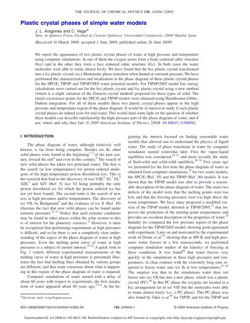
Plastic crystal phases of simple water models
J. L. Aragones and C. Vega a
Dpto. de Química Física, Facultad de Ciencias Químicas, Universidad Complutense, 28040 Madrid, Spain
Received 16 March 2009; accepted 1 June 2009; published online 26 June 2009
We report the appearance of two plastic crystal phases of water at high pressure and temperature
using computer simulations. In one of them the oxygen atoms form a body centered cubic structure
bcc and in the other they form a face centered cubic structure fcc. In both cases the water
molecules were able to rotate almost freely. We have found that the bcc plastic crystal transformed
into a fcc plastic crystal via a Martensitic phase transition when heated at constant pressure. We have
performed the characterization and localization in the phase diagram of these plastic crystal phases
for the SPC/E, TIP4P, and TIP4P/2005 water potential models. For TIP4P/2005 model free energy
calculations were carried out for the bcc plastic crystal and fcc plastic crystal using a new method
which is a slight variation of the Einstein crystal method proposed for these types of solid. The
initial coexistence points for the SPC/E and TIP4P models were obtained using Hamiltonian Gibbs–
Duhem integration. For all of these models these two plastic crystal phases appear in the high
pressure and temperature region of the phase diagram. It would be of interest to study if such plastic
crystal phases do indeed exist for real water. This would shed some light on the question of whether
these models can describe satisfactorily the high pressure part of the phase diagram of water, and if
not, where and why they fail. © 2009 American Institute of Physics. DOI: 10.1063/1.3156856
I. INTRODUCTION
The phase diagram of water, although relatively well
known, is far from being complete. Besides ice Ih, other
solid phases were found at the beginning 1–3 of the past century,
toward the end 4 and even in this century. 5 The search of
new solid phases has taken two principal routes. The first is
the search at low temperatures for proton ordered analogous
of the high temperature proton disordered ices. This is
the research that lead to the discovery of ices VIII, 6 XI, 7 IX, 8
XIII, 5 and XIV Ref. 5 ice VI being probably the only
proton disordered ice for which the proton ordered ice has
not yet been found. The second route is the search of new
ices at high pressures and/or temperatures. The discovery of
ice VII, by Bridgmann 9 and the evidence of ice X Ref. 10
illustrate the fact that new solid phases can be found under
extreme pressures. 11–13 Notice that such extreme conditions
may be found in other places within the solar system so this
is of interest for the planetary sciences. 14 However, it must
be recognized that performing experiments at high pressures
is difficult, and so-far there is not a completely clear understanding
of the aspect of the phase diagram of water at high
pressures. Even the melting point curve of water at high
pressures is a subject of current interest. 15–22 A quick look in
Fig. 1 where different experimental measurements of the
melting curve of water at high pressures is presented illustrates
the fact that melting lines obtained by various groups
are different, and that some consensus about what is happening
in this region of the phase diagram of water is required.
Computer simulations of water started with a delay of
about 60 years with respect to experiments, the first simulations
of water appeared about 40 years ago. 23,24 At the be-
a Electronic mail: cvega@quim.ucm.es.
THE JOURNAL OF CHEMICAL PHYSICS 130, 244504 2009
ginning the interest focused on finding reasonable water
models that allowed one to understand the physics of liquid
water. The study of phase transitions in water by computer
simulation started somewhat later. First the vapor-liquid
equilibria was considered, 25–27 and more recently the study
of fluid-solid and solid-solid equilibria. 28–34 Five years ago
we presented for the first time the phase diagram of water as
obtained from computer simulations, 34 for two water models,
the SPC/E Ref. 35 and the TIP4P Ref. 36 models. It was
shown that the TIP4P model was able to provide a reasonable
description of the phase diagram of water. The main two
defects of the model were that the melting points were too
low, and that the freezing pressures were too high above the
room temperature. We have since proposed a modified version
of the TIP4P model, denoted as TIP4P/2005, 37 that improves
the prediction of the melting point temperatures and
provides an excellent description of the properties of water. 38
Initially we computed the low pressure region of the phase
diagram for the TIP4P/2005 model, showing good agreement
with experiment. Later on and motivated by the experimental
work of Dolan et al. 39 showing that at 400 K and high pressures
water freezes in a few nanoseconds, we performed
computer simulation studies of the kinetics of freezing at
these conditions. It was found 40 that water freezes very
quickly in the simulations at these high pressures and temperatures,
in clear contrast with the extremely long runs required
to freeze water into ice Ih at low temperatures. 41–44
The surprise was that in the simulations water does not
freeze into ice VII but into a new phase, which was a plastic
crystal PC. 40 In this PC phase the oxygens are located in a
bcc arrangement as in ice VII but the molecules were able
to rotate almost freely i.e., a PC phase. This PC phase was
also found by Takii et al. 45 for TIP5P, and for the TIP4P and
0021-9606/2009/13024/244504/14/$25.00 130, 244504-1
© 2009 American Institute of Physics
Downloaded 02 Jul 2009 to 147.96.6.138. Redistribution subject to AIP license or copyright; see http://jcp.aip.org/jcp/copyright.jsp

244504-2 J. L. Aragones and C. Vega J. Chem. Phys. 130, 244504 2009
T (K)
1400
1200
1000
800
600
400
Hemley
Dubrovinskaia
Goncharov
Schwager fit
Schwager data
Datchi
0 10 20 30 40 50
p (GPa)
FIG. 1. Color online Experimental data for the melting curve of the ice
VII. Reference 20: thick solid line and diamonds; Ref. 18: open squares;
Ref. 17: thin solid line; Ref. 16: dashed-dotted line; Ref. 15: open circles.
SPC/E models. Therefore, it seems at this point necessary to
recalculate the high pressure part of the phase diagram of
TIP4P and SPC/E to include this new PC phase that was
overlooked in our previous study. 34 This requires free energy
calculations for the PC phase. In this work we shall describe
in detail how to perform free energy calculations for these
types of solid.
Another issue of interest is the layout of the phase diagram
of these rigid water models TIP4P, TIP4P/2005, and
SPC/E at extremely high pressures. In particular it would be
of interest to establish if a solid with a fcc arrangement of the
oxygens i.e., a close packed structure may appear for these
models at extremely high pressures. 45 As will be shown, this
is indeed the case. A PC phase with a fcc arrangement of the
oxygens appears at high pressures and temperatures, allowing
a better packing of the molecules than the typical bcc
arrangement of ice VII or the bcc PC. These two PC phases
bcc and fcc are also found for the TIP4P and SPC/E models
so that they seem to be present in all water models. In these
models water is described by a Lennard-Jones LJ center
plus additional point charges. At high temperatures, the hydrogen
bond energy in k BT units is not sufficient to maintain
the hydrogen bonding network and the molecules start to
rotate. Once the importance of the charges is reduced, the
relatively spherical shape of water makes the existence of a
PC phase possible. PC phases are also found experimentally
for slightly anisotropic molecules as N 2 or O 2. 46
A word of caution is needed with respect to the conclusions
of this work. Our main goal is to accurately determine
the complete phase diagram of popular water models. Since
these models are used in thousands of simulation studies it is
important to know to what extent they can describe satisfactorily
the phase diagram of water, and where and why they
fail to do so. However, it should be clearly pointed out that
SPC/E, TIP4P, and TIP4P/2005 are rigid models and they
cannot describe properly the formation or the breaking of
chemical bonds. For this reason these models are completely
useless when it comes to understanding the formation of ice
X. In ice X, the oxygens form a bcc lattice and the hydrogens
are located in the middle of the O–O bonds. Also, at ex-
tremely high temperatures a superionic solid has been
proposed 47 where the oxygens form a lattice and the hydrogens
diffuse within the oxygen network. The rigid models of
this work cannot describe these situations. Obviously only
first principle calculations can do that. 47,48 Rather the phase
diagram presented here corresponds to what approximately
would occur in the phase diagram of water in the absence of
deformation or breaking of chemical bonds. It will be shown
that for these models, water adopts close packed structures at
high pressures and PC phases at high temperatures. Whether
real water does indeed form PC phases or fcc solid structures
is an issue that can be solved only by performing experimental
work. Experimental studies proving or disproving the existence
of a PC phase for water, should be of great interest
not only for the people interested in high pressure studies of
water but also for the broad research community performing
computer simulations involving water.
II. SIMULATION DETAILS
We have performed Monte Carlo MC and molecular
dynamics MD simulations for PC phases of water bcc and
fcc. We have used the TIP4P/2005, 37 TIP4P, 36 and SPC/E
Ref. 35 models. They are rigid and nonpolarizable models.
A LJ center is located on the oxygen atom and positive
charges are located on the hydrogen atoms. The negative
charge is located on the H–O–H bisector for the TIP4P models
and on the oxygen for the SPC/E model. In Ref. 38 one
can find a critical comparison of the performance of these
three popular water models.
The number of molecules used in the simulations were
432 for the bcc PC which corresponds to 216 units cells
666, 500 for the fcc PC 125 units cells 555,
432 for ice VII 216 units cells 666, and either 360 or
432 molecules for the fluid phase. In all cases the LJ potential
was truncated at 8.5 Å. Standard long range corrections
to the LJ part of the potential were added. The Ewald summation
technique has been employed for the calculation of
the long range Coulombic forces. We have performed isotropic
and anisotropic NpT simulations. In the isotropic simulations
the volume of the system fluctuates but the shape of
the simulation box remains constant. In anisotropic NpT the
volume and the shape of the simulation box are allowed to
fluctuate. 49,50 For fluid water and for the cubic solids ice VII
and the two PCs we used isotropic scaling. In one case
anisotropic scaling was used for the bcc PC to analyze its
possible transformation into a fcc PC through a Martensitic
phase transition. 51 A typical MC run involves about 30 000
cycles of equilibration and 70 000 cycles to obtain averages
defining a cycle as a trial move per particle plus a trial
volume move.
To determine the phase diagram free energy calculations
are required. Free energy calculations can be determined
with the Einstein crystal method 52–54 or a modified version
denoted as the Einstein molecule approach. 55 The technique
can be used for ices and details have been provided
elsewhere. 56,57 By applying two external fields, one translational
forcing the molecules to occupy a certain position, and
another orientational forcing the molecules to adopt a certain
Downloaded 02 Jul 2009 to 147.96.6.138. Redistribution subject to AIP license or copyright; see http://jcp.aip.org/jcp/copyright.jsp

244504-3 Plastic crystal phases of water J. Chem. Phys. 130, 244504 2009
orientation we have been able to compute the free energy of
a number of solid phases of water. However, the application
of the technique to PCs may be problematic as at low values
of the orientational field very long runs should be performed
to guarantee that the molecules are able to rotate as in the
PC. To avoid this issue we have developed a new method for
free energy calculations of PCs, which allow us to avoid
connecting orientational springs to the molecules. The difference
with the traditional Einstein crystal as applied to other
ices is that for the PCs only translational springs will be
used. The method is inspired in the methodology proposed
by Lindberg and Wang 58 to evaluate dielectric constants of
ices.
An ideal Einstein crystal with the center of mass CM
fixed is used as the reference system to compute the free
energy. Let us describe the different steps to computing the
free energy of a PC:
1 An ideal Einstein crystal is a solid in which the molecules
are bound to their lattice positions by harmonic
springs. For PCs only translational and not orientational
springs will be used this prevents the appearance
of phase transitions along the integration. The
energy of the ideal Einstein crystal is given by
N
U Ein = i=1
Er i − r i0 2 , 1
where ri represents the instantaneous location of the
reference point of molecule i and ri0 denotes its equilibrium
position. UEin is a harmonic field that tends to
keep the molecules at their lattice positions. E is the
coupling parameter of the translational springs and has
units of energy over a squared length. The free energy
of the ideal Einstein crystal with translational springs
CM 53,56
with fixed CM AEin-id is given by
CM CM
AEin-id =−kBT ln QEin,t, 2
3N−1/2
=− kBT lnPCM
N
E 3/2, 3
where PCM =1/ 3N−1N−3/2 and is the thermal De
Broglie wavelength =h 2 /2mkBT1/2, which has
units of length.
2 To the ideal Einstein crystal described above we incorporate
intermolecular interactions in the form of a LJ
potential whose parameters and are identical to
those of the water model under consideration. The difference
in free energy between the Einstein crystal with
CM
LJ interactions AEin-LJ and the noninteracting Einstein
CM
crystal AEin-id both with fixed CM can be obtained in
a perturbative way as
CM CM
A1 = AEin-LJ − AEin-id
= U lattice − k BT lnexp− U sol − U lattice Ein-id,
4
where U lattice is the energy of the system when the molecules
stand fixed on the lattice position i.e., the LJ
lattice energy and U sol is the LJ energy of the system
for the considered configuration. The average is performed
over configurations generated for the ideal
Einstein crystal.
3 Then we evaluate the free energy difference between an
Einstein crystal with water interactions i.e., TIP4P/
2005, SPC/E, etc. and an Einstein crystal with LJ interactions,
both with fixed CM. To evaluate this free
energy difference, the charges of the water potential are
turned on, while keeping the translational springs. The
path linking the LJ potential to the water potential is
defined as
U Q = 1− QU LJ + QU water, 5
1
CM CM
AQ = AEin-sol − AEin-LJ = Uwater − ULJN,V,T,Qd Q,
0
6
where U water−U LJ N,V,T,Q can be obtained in a NVT
simulation at a given Q. As the reference LJ potential
has the same parameters as the LJ part of the water
potential then U water−U LJ N,V,T,Q is simply the Coulombic
contribution to the energy of the water potential
U Q and Eq. 2 can be rewritten as
A Q = 0
1
U Q N,V,T,Q d Q. 7
Since we are not using orientational springs the molecules
are able to rotate at the beginning when Q=0 and at the end when Q=1 of the integration avoiding
the possible existence of a phase transition along the
integration path. The value of the integral is then obtained
numerically.
4 Now the translational springs are turned off gradually.
The free energy change A2 between the water molecules
bonded to their lattice positions by harmonic
CM
springs AEin-sol and the PC with no translational
springs both with fixed CM is given by
CM CM
A2 = Asol − AEin-sol =−0 E UEin-id N,V,T,
E
d E.
8
Since the integrand changes by several orders of magnitude
it is convenient to perform a change in
variable 52,59 from E to ln E+c, where c is a constant.
We shall use c=exp3.5 which significantly
smoothes the integrand. The final expression for A 2 is
A 2 =− lnc
ln E +c UEin-id N,V,T, E + c
E
dln E + c. 9
Fixing the CM avoids the quasidivergence of the integrand
of Eq. 9 when the coupling parameter tends
to zero. Without this constraint, the integrand would
increase sharply in this limit, making the evaluation of
the integral numerically involved.
Downloaded 02 Jul 2009 to 147.96.6.138. Redistribution subject to AIP license or copyright; see http://jcp.aip.org/jcp/copyright.jsp

244504-4 J. L. Aragones and C. Vega J. Chem. Phys. 130, 244504 2009
(5) The last step is to evaluate the free energy change between
a PC with no constraint and the PC with a fixed
CM. The free energy change in this last step A3 is
given by
CM
A3 = Asol − Asol =−kBT ln Qsol CM
Qsol = k BTlnP CM /P −lnV/N, 10
where P=1/ 3N . A 3 does not depend on the particular
form of the intermolecular potential U sol.
The final expression of the free energy of the PC is
CM
Asol = AEin-id + A3 + A1 + AQ + A2 = A 0 + A 1 + A Q + A 2. 11
CM
Placing together the AEin-id and A3 terms A0, the PCM contribution cancels out and the final expression of the free
energy of the PC solid is
A sol
Nk BT
=− 1
N
ln 1
+ U lattice
Nk BT
3N
E
3N−1/2
+ 1 0
UQ dQ NkBTN,V,T, Q
− 1 0
UEin-id NkBTN,V,T, N
3/2 V
N
− 1
N lnexp− U sol − U lattice Ein-id
d. 12
The first term corresponds to A 0, the second to A 1, the third
to A Q, and the last term to A 2.
The free energy was computed at a certain thermodynamic
state. By using thermodynamic integration the free
energy for other thermodynamic conditions can be obtained
easily. The free energy of the fluid phase was obtained as
described in our previous work. 56 The chemical potential is
easily obtained as /k BT=G/Nk BT=A/Nk BT+pV/Nk BT.
Once the free energies and chemical potentials for the fluid
and for the different solid phases are known initial coexistence
points can be located by imposing the condition of
equal chemical potential I= II at the same temperature
and pressure. Having an initial coexistence point the rest of
the coexistence curve can be obtained by using Gibbs–
Duhem integration. 60,61 This technique allows one to determine
the coexistence line between two phases, provided that
an initial coexistence point is known. Gibbs–Duhem is a numerical
integration of the Clapeyron equation and where
volume and enthalpy changes are obtained by using computer
simulations. The Clapeyron equation is given by
dp
dT = sII − sI =
vII − vI hII − hI . 13
TvII − vI Subscripts I and II label the corresponding phases and the
thermodynamic properties written with small letters are
properties per particle x=X/N. For the integration of the
Clapeyron equation a fourth-order Runge–Kutta integration
is employed.
In this work free energy calculations were performed
only for the TIP4P/2005 model. To obtain initial coexistence
points for the TIP4P and SPC/E models of water we shall use
Hamiltonian Gibbs–Duhem integration. Hamiltonian Gibbs–
Duhem integration is a very powerful technique that allows
one to determine the change in the coexistence conditions of
a certain coexistence line due to a change in the water potential.
In this kind of integration the Hamiltonian of the
system is changed through a coupling parameter so that
=0 for the initial Hamiltonian and =1 for the final Hamiltonian.
When the coupling parameter is introduced
within the expression of the potential energy of the system
U, then a set of generalized Clapeyron equations can be
derived. The derivation is as follows. For two phases at coexistence,
g IT,p, = g IIT,p,. 14
If the system is perturbed slightly while preserving the
coexistence it must hold that
− s IdT + v Idp + g I
d =−s IIdT + v IIdp + g II
d.
15
If the coupling parameter remains constant when performing
the perturbation then one recovers the traditional Clapeyron
Eq. 13coexistence on the p-T plane. If the pressure is kept
constant when the perturbation is performed coexistence on
the -T plane then one obtains
dT
d =
T gII − gI
. 16
hII − hI The property g/=u/ N,p,T,, can be determined
easily during the NpT simulations. Then Eq. 16 can
be rewritten as
dT
d =
T uII − uI
. 17
hII − hI This generalized Clapeyron Eq. 16 can be integrated numerically
from =0 to =1 to obtain the coexistence temperature
at a certain fixed pressure of the water potential of
interest, provided that the coexistence temperature is known
for the initial reference potential.
A similar equation can be obtained when a perturbation
is performed while keeping the temperature constant. In
this case the coexistence pressure of the water potential of
interest is obtained at a certain fixed temperature provided
that the initial coexistence pressure is known for the initial
reference potential. The working expression is
dp
d =− uII − uI
. 18
vII − vI Downloaded 02 Jul 2009 to 147.96.6.138. Redistribution subject to AIP license or copyright; see http://jcp.aip.org/jcp/copyright.jsp

244504-5 Plastic crystal phases of water J. Chem. Phys. 130, 244504 2009
Let us assume that is as a coupling parameter leading
the system from a certain reference potential UA to the potential
of interest UB. This can be done with a coupling of the
form,
U = UB + 1−UA, 19
with changing from zero initial reference potential to one
final potential of interest. The generalized Clapeyron equations
can be written as
dT
d = Tu II
I
B − uAN,p,T, − uB − uAN,p,T, , 20
hII − hI dp
d =−u II
I
B − uAN,p,T, − uB − uAN,p,T, , 21
vII − vI where uB is the internal energy per molecule when the interactions
between molecules are described by UB and analogous
definition is used for uA. If a coexistence point between
two phases is known for potential A then integration of the
previous equations from =0 to =1 allows one to determine
the coexistence point between these two phases for
potential B. This can be done either by fixing the temperature
or the pressure along the integration.
To estimate nucleation times of the PC phases and to
determine the melting point of the fcc PC phase by direct
coexistence technique we have performed MD simulations
using the program GROMACS. 62 In these simulations the temperature
is kept constant by using a Nose–Hoover
thermostat 63,64 with a relaxation time of 2 ps. To keep the
pressure constant, a Parrinello–Rahman barostat 49,51 isotropic
or anisotropic was used. The relaxation time of the
barostat was 2 ps. The time step was 1 fs and the typical
length of the runs was of about 5 ns. The geometry of the
water molecules is enforced using constraints. The LJ part of
the potential was truncated at 8.5 Å and standard long range
correction were added. Ewald sums are used to deal with the
long range Coulombic interactions. Coulombic interactions
in real space were truncated at 8.5 Å. The Fourier part of the
Ewald sums was evaluated using the particle mesh Ewald. 65
The width of the mesh was 1 Å and we used a fourth order
interpolation.
III. RESULTS
For the TIP4P/2005 model we found in previous work
that ice VII transformed into a bcc PC at 377 K when heated
along 70 000 bars isobar. 40 We shall now explore the stability
of this bcc PC. It is well known that a bcc solid can transform
into a fcc solid, provided that the fcc is more stable,
and that one uses anisotropic NpT simulations Rahman–
Parrinello NpT. We shall explore the behavior of the bcc PC
solid when heated along the 70 000 bars isobar. The bcc PC
is stable when heating up to temperatures of about 460 K
even though we are using anisotropic NpT simulations and
it could transform into a fcc solid but at 480 K the properties
of the system energies, densities, and shape of the simulation
box undergo a clear jump. A Martensitic phase transition
occurs in which the bcc lattice is transformed into a fcc
lattice by increasing the c edge of the bcc structure. The
z
(a)
(b)
(c)
A
y
x
a
2a
a
2a
a
H
θ
2a
a
2a
a
H
2a
H
simulation box that was originally cubic for the bcc PC becomes
tetragonal a sketch of the transformation is given in
Fig. 2. In Fig. 3 the instantaneous values of the lengths of
the sides of the simulation box are presented for a temperature
of 440 K and for a temperature of 480 K. As can be seen
at 440 K one sees fluctuations of three sides of identical in
average lengths. However, for the run performed at 480 K
one of the sides increases slightly its length at the beginning
of the run and after 40 000 cycles increases its length dramatically.
At the end of the 480 K run the length of the sides
are a=17.608: b=17.620; c=25.557. As can be seen the ratio
c/a is close to c/a=21.414, which is the value expected
for the ratios of c and a in a Martensitic transformation from
a bcc to a fcc solid see the sketch of Fig. 2. Therefore, the
ratio c/a actually the ratio between the longest and the
shortest sides of the simulation box since the Martensitic
θ
H
2a
2a
FIG. 2. Color online a Two bcc unit cells. b How the fcc lattice can be
obtained from two bcc cells. When the z direction is scaled by 2a, the
crystal is transformed into a fcc lattice. c fcc unit cell.
Downloaded 02 Jul 2009 to 147.96.6.138. Redistribution subject to AIP license or copyright; see http://jcp.aip.org/jcp/copyright.jsp

244504-6 J. L. Aragones and C. Vega J. Chem. Phys. 130, 244504 2009
Box sides (Å)
(a)
Box sides (Å)
(b)
30
25
20
15
0 20000 40000 60000
MC cycles
30
25
20
Side a
Side b
Side c
Side a
Side b
Side c
15
0 20000 40000 60000
MC cycles
70000 bar
440 K
70000 bar
480 K
FIG. 3. Color online Simulation box sides change along the MC run anisotropic
NpT ensemble for the bcc PC phase. a 440 K and 70 000 bars.
b 480 K and 70 000 bars.
transition may occur also along the x or y axis is a good
order parameter to detect the transformation. In Fig. 4 the
c/a ratio is plotted as a function of temperature for runs
performed along the 60 000, 70 000, and 80 000 bars isobars.
For the pressure 60 000 bars no bcc to fcc transition is observed.
For the runs at 70 000 bars the transition occurs at
c/a
1.4
1.2
1
60000 bar
70000 bar
80000 bar
1.414
400 450 500 550 600
T (K)
FIG. 4. Color online Temperature dependence of the c/a ratio at different
pressures, 60 000 bars open circles, 70 000 bars open squares, and
80 000 bars open diamonds.
g (r O-O )
4
3
2
1
0
2 4 6 8
r (Å)
O-O
about 480 K. For the runs at 80 000 bars the transition occurs
at about 420 K. Therefore the transition temperature decreases
as the pressure increases. That suggests a negative
slope of the bcc-fcc coexistence line. Notice that the jump in
Fig. 4 does not correspond to the true coexistence point i.e.,
identical chemical potential between these two phases.
Packing considerations favor the fcc structure with respect to
the bcc structure. In fact for a r −12 potential Wilding 66 found
recently that the fcc structure is more stable than the bcc.
We have found that the fcc PC could also be generated
easily by starting from a fcc arrangement of the oxygen atoms
and introducing random orientations. In fact we generated
the fcc PC starting from a fcc solid of 500 molecules
i.e., 125 unit cells. In Fig. 5 the oxygen-oxygen radial distribution
function g O–O is shown. As can be seen the radial
distribution function of the solid obtained from the Martensitic
transformation is identical to that obtained from an initial
fcc arrangement of oxygens. The radial distribution function
of the fcc PC is clearly different from that of the bcc PC.
In fact the bcc PC shows the first peak of the g O–O at 2.81 Å,
the second at 4.59 Å, and the third at 5.50 Å, whereas fcc PC
has a first peak at 2.87 Å and the second and third peaks
move apart and shift to shorter distances, 4.16 and 5.10 Å,
respectively Fig. 5.
We have computed the powder x-ray and neutron diffraction
patterns. The intensity of the diffraction peaks is
obtained as
I=
fcc obtained by heating a bcc PC
fcc obatined by initial fcc arrangements of oxygens
bcc plastic crystal
FIG. 5. Color online Oxygen-oxygen radial distribution functions at T
=440 K and p=80 000 bars for the fcc PC phase and at T=440 K and p
=70 000 bars for the bcc PC. fcc PC obtained by heating the bcc PC solid
line, fcc PC obtained by the fcc lattice of the oxygens filled circles, and
bcc PC dashed-dotted line. Notice that the correct g O–O and g O–H in Figs.
2, 4, and 5 of our previous work Ref. 40 are obtained by shifting the
curves 0.5 Å to the right.
P
sensen2 m iF hkl 2 , 22
where m i is the multiplicity and P is the polarization factor
in neutron diffraction P=1 and in x-ray diffraction
P=1+cos 2 2/2. In the x-ray diffraction pattern, the
F hkl is obtained as
Downloaded 02 Jul 2009 to 147.96.6.138. Redistribution subject to AIP license or copyright; see http://jcp.aip.org/jcp/copyright.jsp

244504-7 Plastic crystal phases of water J. Chem. Phys. 130, 244504 2009
Intensity / a. u.
(a)
Intensity / a.u.
(b)
25000
Ice VII
bcc PC
20000
15000
10000
5000
0
5
10
15
20
2 θ / degrees
25 30
Fhkl = 1
N N
fne n=1
2ihxn +kyn +lzn , 23
where f n is function of . Both oxygen and hydrogens
were considered and f n was obtained from the fit proposed
by Lee and Pakes. 67 The wavelength used was
0.4 Å. 11,13 In the neutron diffraction pattern which was calculated
for heavy water F hkl was obtained as
F hkl = 1
N
011
011
002 002
112
112
7000
6000
Ice VII
bcc PC
5000
4000
3000
2000
1000
0
5
10
15
20
2 θ /degrees
25
30
011
011
111
111
112
FIG. 6. Color online a Simulated powder x-ray diffraction pattern for ice
VII dashed line at 70 000 bars and 300 K and bcc PC solid line at 70 000
bars and 400 K. The wavelength used was 0.4 Å. The Miller indices hkl are
given for each peak. b Simulated neutron diffraction pattern for ice VII
dashed line at 70 000 bars and 300 K and bcc PC solid line at 70 000
bars and 400 K. The wavelength was 0.4 Å. The Miller indices hkl are given
for each peak.
N bne n=1
2ihxn +kyn +lzn , 24
where the neutron scattering amplitudes b n of the deuteron
and the oxygen atom are 0.6671 and 0.5803 fm, respectively,
and do not depend on . 68 The wavelength used was also
0.4 Å. The number of molecules used in these simulations
were 1024 512 unit cells and we checked that the bcc PC
also appears for this system size. Results are presented in
Fig. 6. The main difference between the ice VII and bcc PC
x-ray diffraction patterns is the intensity reduction, around
20%, for the bcc PC peaks and the appearance of more peaks
at large 2 values for the bcc PC. The same results are ob-
022
022 022
122
013
222
222
123
123
033 033
served on the neutron diffraction pattern Fig. 6b. The intensity
reduction of the diffraction peaks is not surprising if
one takes into account that in ice VII the hydrogen bonds
maintain the location of the oxygen atoms more or less fixed
except for some slight thermal vibration. However in the
PC phases the molecules are free to rotate frequently forming
and breaking hydrogen bonds so the oxygen atom is
able to move significantly from its equilibrium lattice position.
The bcc PC diffraction peaks were shifted to lower 2
values with respect to ice VII due to the lower density of this
phase. The conclusion of these results is that one of the signatures
of the formation of a PC phase say the bcc will be
a significant reduction in the intensity of the diffraction lines
with respect to ice VII. Observing the intensity ratio between
the 011 and 111 peaks I 011/I 111 on the neutron diffraction
pattern for ice VII and bcc PC, we can see that its value is of
about 4 for ice VII and of about 15 for bcc PC. Therefore the
ratio I 011/I 111 could be used to detect the appearance of the
bcc PC.
To gain further understanding of the orientational order
in the PC phases we have also determined the probability
distribution of the polar angles and of the OH bonds.
The x axis is located on the a vector of the unit cell, the y
axis is located on the b vector of the unit cell, and the z axis
is located along the c vector of the unit cell see Figs. 2a
and 2c. The distribution function f is defined as
f = N
, 25
2N
where N denotes the number of OH bonds with polar
angle between and + and 2N is the number of OH
bonds i.e., twice the number of molecules N. The distribution
function f is defined as
f = N
. 26
2N
In Fig. 7 the functions f and f are presented for ice
VII at 300 K and 70 000 bars, bcc PC at 400 K and 70 000
bars and fcc PC at 440 K and 80 000 bars. For the PC
phases, bcc and fcc, the distribution functions f and f
are more uniform than those of ice VII. This is due to the fact
that in the PC phases the molecules are able to rotate almost
freely. Nevertheless the angular distribution is not uniform
even in the PC phase since the OH vectors still prefer to
point out to the contiguous oxygen atoms. For bcc PC and
ice VII the peaks of f are located at 54.74 and 180
54.74 where 54.74 is the angle between one of the diagonals
of the cube and a line connecting the center of two
opposite faces Fig. 2a. However, for the fcc PC the peaks
of f are located at 45°, 90°, and 135°. Where 45 and 135
are the angles between one of the diagonals that is connecting
the center of two perpendicular faces of the cube and the
z edge Fig. 2c and 90 is the angle between the line connecting
two oxygens resting on the same plane with the z
edge. For the bcc PC the angles 0°, 90°, and 180° in the f
have nonzero probability. This provides some indication that
in the bcc PC the OH vectors point sometimes while rotating
to second nearest neighbors. For ice VII and the bcc PC,
Downloaded 02 Jul 2009 to 147.96.6.138. Redistribution subject to AIP license or copyright; see http://jcp.aip.org/jcp/copyright.jsp

244504-8 J. L. Aragones and C. Vega J. Chem. Phys. 130, 244504 2009
f(θ)
(a)
f(φ)
(b)
0.03
0.025
0.02
0.015
0.01
0.005
0.012
0
0 50 100 150 200
θ (degrees)
0.01
0.008
0.006
0.004
0.002
0
0 100 200 300
φ (degrees)
Ice VII
Plastic crystal bcc
Plastic crystal fcc
Ice VII
Plastic crystal bcc
Plastic cristal fcc
FIG. 7. Color online a f as a function of angle for ice VII dasheddotted
line at 300 K and 70 000 bars, for the bcc PC dashed line at 400 K
and 70 000 bars and for the fcc PC solid line at 440 K and 80 000 bars. b
f as a function of angle for the ice VII dashed-dotted line at 300 K
and 70 000 bars, for the bcc PC dashed line at 400 K and 70 000 bars and
for the fcc PC solid line at 440 K and 80 000 bars.
the angular distribution f presents four peaks separated
by 90° as should be the case. In the fcc PC the function f
is almost uniform, indicating that the molecules can rotate
quite freely. For ice VII at 300 K and 70 000 bars and for the
length of the simulations performed in this work, a certain
individual molecule presents a fixed value of and subject
to some thermal vibration. However for the PC phases
each individual molecule jumps quite often from one of the
peaks of the distribution to another peak. These flipping or
jumping moves occur quite often for each molecule within
the length of the simulation runs considered here. Another
way to see this orientational disorder is by means of the
visualization of the MD trajectories. Multimedia mpg files
for the MD trajectories of ice VII, bcc PC, and fcc PC are
provided as electronic supplementary information. 69
Let us now determine coexistence points between the
different solid phases considered in this work fluid, ice VII,
bcc PC, and fcc PC. This requires free energy calculations
for the different phases involved. Free energies for the liquid
and for ice VII were obtained in our previous work. 40 We
have determined the Helmholtz free energy for the bcc PC
and fcc PC at 440 K and for the densities which correspond
to that of the systems at 80 000 bars. The free energies are
TABLE I. Helmholtz free energy for ice VII, bcc PC phase, and fcc PC
phase as obtained with the Einstein crystal methodology. The Gibbs free
energy was computed after adding pV to the Helmholtz free energy. The
density is given in g/cm 3 . The cubic fcc* phase correspond to the fcc PC
phase obtained by heating the bcc PC phase.
Phase Molecules T K P bar A/Nk BT G/Nk BT
Ice VII 432 300 70 000 1.707 9.75 19.87
Cubic bcc 432 440 80 000 1.662 3.93 19.78
Cubic fcc 500 440 80 000 1.679 4.86 19.23
Cubic fcc* 432 440 80 000 1.679 4.89 19.21
Cubic fcc 500 440 105 000 1.749 3.76 25.80
presented in Table I. For the fcc solid we have computed the
free energy for a cubic simulation box 500 molecules and
for the tetragonal simulation box obtained from the Martensitic
transition of the bcc PC 432 molecules. As can be seen
the free energy of these two systems is the same. The small
difference may be attributed to the different orientations of
the crystallographic planes with respect to the periodic
boundary conditions. 70 For the studied thermodynamic state
80 000 bars and 440 K, the fcc PC is more stable than bcc
TABLE II. Melting curves of the PC phases of the TIP4P/2005 as obtained
from free energy calculations and Gibbs–Duhem integration with isotropic
NpT simulation performed for the fluid and for the PC phases. The densities
are given in g/cm 3 . The residual internal energies are given in kcal/mol. The
* indicate the initial coexistence point.
T K p bar U 1 U 2 1 2
Fluid-bcc PC
340.00 60 193 10.45 10.03 1.574 1.622
* 400.00 62 000 9.87 9.58 1.562 1.609
440.00 64 390 9.52 9.30 1.564 1.608
460.00 66 042 9.35 9.12 1.560 1.607
520.00 71 653 8.86 8.71 1.563 1.615
↓ Metastable
600.00 80 608 8.20 8.13 1.575 1.626
700.00 93 249 7.38 7.37 1.599 1.646
900.00 121 380 5.77 5.92 1.636 1.690
1000.00 137 036 4.96 5.15 1.657 1.713
Fluid-fcc PC
* 440.00 66 790 9.52 9.06 1.575 1.628
500.00 70 691 9.00 8.67 1.566 1.629
520.00 72 435 8.86 8.54 1.569 1.629
540.00 74 164 8.68 8.44 1.575 1.633
560.00 76 115 8.56 8.29 1.569 1.635
↑ Metastable
600.00 80 089 8.21 8.03 1.571 1.639
650.00 85 533 7.83 7.71 1.581 1.648
700.00 91 508 7.44 7.37 1.590 1.657
720.00 93 955 7.30 7.21 1.593 1.661
740.00 96 444 7.14 7.09 1.597 1.663
760.00 98 973 6.96 6.97 1.599 1.667
780.00 101 586 6.81 6.80 1.602 1.672
800.00 104 216 6.66 6.67 1.607 1.677
900.00 118 027 5.85 5.99 1.625 1.698
1000.00 132 701 5.10 5.28 1.649 1.719
Downloaded 02 Jul 2009 to 147.96.6.138. Redistribution subject to AIP license or copyright; see http://jcp.aip.org/jcp/copyright.jsp

244504-9 Plastic crystal phases of water J. Chem. Phys. 130, 244504 2009
TABLE III. Solid-solid coexistence lines of the TIP4P/2005 model for the
high pressure polymorphs ice VII, PC bcc and PC fcc as obtained from
free energy calculations and Gibbs–Duhem integration. The densities are
given in g/cm 3 . The internal energies in kcal/mol only the residual part of
the internal energy is reported. The* indicate the initial coexistence point.
T K p bar U 1 U 2 1 2
VII-bcc PC
600.00 250 304 4.13 3.54 1.979 1.972
550.00 190 835 6.11 5.50 1.902 1.889
500.00 143 221 7.67 7.04 1.828 1.810
440.00 101 354 8.99 8.49 1.749 1.728
400.00 80 146 9.76 9.19 1.707 1.674
↑ Metastable
* 377.00 70 000 10.04 9.53 1.681 1.645
360.00 63 292 10.27 9.79 1.666 1.623
350.00 59 665 10.40 9.95 1.656 1.617
VII-fcc PC
* 393.00 77 179 9.94 9.04 1.703 1.677
414.75 100 000 9.17 8.34 1.752 1.740
446.94 200 000 6.73 5.43 1.938 1.935
441.29 400 000 1.19 0.41 2.162 2.168
422.43 500 000 1.61 3.29 2.244 2.251
400.00 592 309 4.18 5.87 2.309 2.319
300.00 880 106 12.12 13.76 2.474 2.489
250.00 980 523 14.81 16.41 2.523 2.539
bcc PC-fcc PC
* 570.00 77 124 8.35 8.22 1.621 1.635
520.00 74 646 8.65 8.51 1.625 1.639
500.00 74 495 8.75 8.61 1.630 1.643
460.00 74 746 8.97 8.78 1.640 1.655
440.00 75 551 9.03 8.85 1.648 1.661
400.00 78 266 9.20 8.98 1.666 1.679
380.00 80 876 9.44 9.02 1.691 1.692
PC it has a lower chemical potential. This is consistent with
the results presented in Fig. 4 where it was shown that when
anisotropic NpT simulations were used the bcc PC transformed
into a fcc PC. Notice however that it is possible to
have a mechanically stable bcc PC at 80 000 bars and 440 K
provided that isotropic NpT simulations are performed with
this type of scaling the bcc PC remains mechanically stable
so it is possible to compute thermodynamic properties even
under conditions where the solid is metastable from a thermodynamic
point of view. In Table I the free energy is presented
for two different thermodynamic states of the fcc PC.
By using thermodynamic integration it is possible to estimate
the free energy at 440 K and 105 000 bars starting from the
value at 440 K and 80 000 bars. We obtain −3.77Nk BT which
is good agreement with the value −3.76Nk BT obtained from
Einstein crystal calculation Table I.
By using thermodynamic integration the coexistence
point between the fluid and the fcc PC has been located at
440 K and 66 790 bars. Once an initial coexistence point has
been found for the fluid-fcc PC transition, the rest of the
coexistence line will be obtained by Gibbs–Duhem integration.
The fluid-bcc PC was integrated from the coexistence
point given in our previous work at 400 K and 62 000 bars,
TABLE IV. New triple points for the TIP4P/2005, TIP4P, and SPC/E models.
The rest of the triple points of the models were given in Refs. 40 and 71.
Phases
TIP4P/2005 TIP4P SPC/E
T K p bar T K p bar T K p bar
L-VII-bcc 352 60 375 322 58 929 347 71 284
L-bcc-fcc 570 77 124 520 73 100 683 103 426
VII-bcc-fcc 393 77 179 363 76 091 434 112 204
obtained by free energy calculations. The fluid-bcc PC and
fluid-fcc PC coexistence lines meet at a triple point located
around 570 K and 77 124 bars. This triple point can be used
as initial coexistence point of the bcc PC-fcc PC coexistence
curve. This curve intersects the ice VII-bcc PC coexistence
line, generating a new triple point at 393 K and 77 179 bars.
This triple point was used as initial point for the ice VII-fcc
PC coexistence line. The new coexistence lines for the
TIP4P/2005 model are given in tabular form in Tables II and
III. The triple points generated by these coexistence lines are
shown in Table IV. The rest of the triple points of these
models can be found in Refs. 40 and 71.
Free energy calculation is somewhat involved and it is
convenient to determine coexistence points by an independent
procedure. For this reason we also used direct coexistence
simulations to determine the fluid-fcc PC transition.
The direct coexistence technique, was pioneered by Woodcok
and co-workers. 72–74 An equilibrated configuration of a
fcc PC phase 500 molecules was located on the left hand
side of the simulation box and put into contact with an
equilibrated configuration of the fluid having 500 molecules.
We then performed MD simulations using GROMACS, while
keeping the temperature at 600 K. We performed several
runs at different pressures. In Fig. 8, the evolution of the
density with time is shown for several pressures. As we can
see, for low pressures 70 000 and 79 000 bars the density
decreases indicating the melting of the fcc PC. For high pressures
80 500 and 90 000 bars the density of the system
Density (Kg m -3 )
1750
1700
1650
1600
1550
70000 bar
79000 bar
80500 bar
90000 bar
0 50 100 150 200
Time (ps)
FIG. 8. Color online Evolution of the density with the time as obtained
from direct coexistence MD simulations. All results were obtained for T
=600 K. Lines from the top to the bottom correspond to the pressures
90 000, 80 500, 79 000, and 70 000 bars, respectively. For the two first
pressures the liquid water freezes, whereas for the last two pressures the
solid melts. The estimate coexistence pressure at 600 K is 79 750 bars.
Downloaded 02 Jul 2009 to 147.96.6.138. Redistribution subject to AIP license or copyright; see http://jcp.aip.org/jcp/copyright.jsp

244504-10 J. L. Aragones and C. Vega J. Chem. Phys. 130, 244504 2009
p(bar)
1e+06
1e+05
10000
1000
II
VIII
VI
I h
A 1e+06
p (bar)
1e+05
VIII
10000
1000
increases indicating the freezing of the fluid into a fcc PC.
This gives a coexistence pressure of about 79 750 bars. Thus,
the value of about 80 000 obtained from free energy calculations
is consistent with the results obtained from direct
coexistence.
Dolan et al., 39,75 showed that the formation of a high
pressure ice phase from liquid water occurs in a few nanoseconds
when the temperature is around 400 K. By using
computer simulations we obtain further evidence of this by
nucleating the bcc PC solid from the fluid in a few
nanoseconds. 40 This nucleation time is small compared to
that found previously for ice Ih Ref. 41 hundreds of nanoseconds.
We will attempt here to nucleate the fcc PC solid.
We performed MD simulations of the fluid phase with isotropic
scaling using 500 molecules in a cubic simulation box
500 molecules is the number of water molecules required to
form 125 unit cells of the fcc PC 4555. The simulations
were performed at 600 K and 100 000 bars where the
fcc PC is the thermodynamically stable phases. No nucleation
of the fcc PC was observed after 12 ns. We then
changed strategy and performed, with the same conditions,
MD simulations with isotropic scaling of the sides of the
simulation box, using a cubic box, containing 432 molecules.
V
(a)
VII
III
II
Ih
VI
V
VII fcc PC (XVI?)
III
bcc PC (XV?)
Liquid
0 100 200 300 400 500 600 700 800
T (K)
0 200 400 600 8000
200 400 600 800
(b) (c)
T (K)
fcc plastic crystal
Fluid
VIII
II
I h
VI
V
VII bcc
plastic crystal
III
T (K)
FIG. 9. a Global phase diagram for the TIP4P/2005 model. b What the phase diagram for the TIP4P/2005 model would be like if the bcc PC phase would
be excluded. c What the phase diagram for the TIP4P/2005 model would be like if the fcc PC phase would be excluded.
Fluid
1e+06
1e+05
10000
1000
p (bar)
This number of molecules 432 corresponds to 216 unit
cells of a bcc PC 2666. In this case we observed
in most of the cases the formation of a bcc PC in a few
nanoseconds in fact the oxygen-oxygen radial distribution
function was clearly that of the bcc PC. With this bcc PC
nucleated from the fluid we then performed anisotropic NpT
MD simulations. In most of the cases nothing happened, but
in one of the runs the bcc PC transformed into a fcc PC
through a Martensitic transformation. This typically occurred
when the bcc PC obtained was free of defects and with their
crystallographic axis aligned with the vectors of the simulation
box. The overall picture is that the formation of the fcc
PC from the fluid occurs in two steps. First, the bcc PC is
formed. Then the bcc PC is transformed into the fcc PC via
a Martensitic transition. This two step process is the most
likely path to the nucleation of the fcc PC. It seems clear that
the free energy nucleation barrier for the formation of the bcc
PC from the fluid is lower than the nucleation barrier for the
formation of the fcc PC from the fluid. 76
The results of this work make it possible to plot for the
first time the complete phase diagram of the TIP4P/2005
model. This is presented in Fig. 9a. The model provides a
qualitatively correct description of the phase diagram of wa-
Downloaded 02 Jul 2009 to 147.96.6.138. Redistribution subject to AIP license or copyright; see http://jcp.aip.org/jcp/copyright.jsp

244504-11 Plastic crystal phases of water J. Chem. Phys. 130, 244504 2009
ter see the correct location of ices Ih to VI. It is seen that
the two PCs dominate the phase diagram of the TIP4P/2005
model of water for temperatures above 400 K. The bcc PC to
fcc PC transition presents a small negative slope. The slopes
of the melting curves of the bcc PC and of the fcc PC are
quite similar and relatively small compared to the slope in
the melting curve of the rest of the ices. In fact we found a
slope of the melting curve of the PC solids of about 100
bars/K at temperatures around 550 K. This slope is smaller
than the slope found in the melting curve of ices Ih, III, V,
VI, and VII. In Fig. 9 lower panel the phase diagrams of
the TIP4P/2005 are presented when the bcc PC Fig. 9b or
fcc plastic Fig. 9c are not considered. These are virtual
phase diagrams since for the TIP4P/2005 the fcc PC or bcc
PC do indeed exists and the true phase diagram of the model
is that of the upper panel. The purpose of the diagram of the
Fig. 9c is to show that the coexistence curve between ice
VII and the bcc PC always presents a positive slope. In other
words ice VII is always more dense than the bcc PC at a
given temperature and pressure. This is not surprising since
both phases present the same arrangement of oxygen atoms,
but the localized character of the hydrogen bonds in ice VII
provokes a higher density. We do not expect any change in
the sign of the slope in the coexistence line between ice VII
and the bcc PC. However, in Fig. 9b we see a change in
slope in the transition between ice VII and the fcc PC. At low
pressures ice VII is more dense than the fcc PC the stronger
hydrogen bonds in ice VII compensate the less efficient
packing of molecules in the bcc arrangement. However the
VII-fcc PC presents re-entrant behavior. In fact a high pressures
the fcc PC is more dense than ice VII. This is further
illustrated in Fig. 10a where the equation of state of ice VII
and of the fcc PC at 300 K are shown, from pressures of
about 70 000 to extremely high pressures. The crossing in
the densities is clear. Notice that the crossing does not indicate
any phase transition. The black filled circles in Fig.
10a indicate the coexistence point as obtained from Gibbs–
Duhem simulations. At sufficiently high pressures the more
efficient packing of the fcc arrangement of oxygens dominates
the physics of the model. The density of the bcc PC is
intermediate between that of the fluid and that of ice VII at
the same T and p Fig. 10b. The physics of PC has been
discussed before for simple models 77 such as hard diatomic
molecules. 78–85
Let us now analyze if the PC phases also appear in other
water models such as TIP4P and SPC/E. Although we computed
the phase diagram for these two models in our previous
work 34 it seems necessary to recalculate the upper part of
the phase diagram for at least two reasons. First because we
did not consider the possibility of having plastic PC phases
in the phase diagram. Second because the free energy calculations
for ice VII were performed at a temperature and pressure
where the system was already in a PC phase 443 K and
a pressure of about 78 350 bars. Therefore our free energy
calculations for ice VII reported recently in Ref. 56 of the
TIP4P and SPC/E were incorrect. The rest of free energies
and coexistence lines are correct. By performing Hamiltonian
Gibbs–Duhem integration we estimate an initial coexistence
point for the coexistence lines involving ice VII and
V M (cm 3 mol -1 )
(a)
p (bar)
0.55
0.5
0.45
0.4
1e+05
90000
80000
70000
60000
50000
Ice VII
fcc plastic crystal
10 20 30 40 50 60 70 80 90 100
p (GPa)
Ice VII
Liquid water
bcc PC
Fluid
bcc PC
Ice VII
1.45 1.5 1.55 1.6 1.65 1.7 1.75
ρ (g cm -3 40000
(b)
)
FIG. 10. Color online a Equation of state of ices VII solid line and fcc
PC crosses for 300 K as obtained from computer simulation for TIP4P/
2005 model. Lines indicate thermodynamic stable phase for each pressure.
For low pressures the solid line corresponds to ice VII. At high pressures the
dashed line with crosses corresponds to fcc PC. The coexistence point between
the two ices is given by the filled circles. b Equation of state of ice
VII thin solid line, bcc PC dashed line, and liquid water thick solid line
for 380 K as obtained by computer simulation for TIP4P/2005 model. The
dotted lines gives the coexistence.
the PC phases. Once this initial point was located the rest of
the coexistence line was obtained by Gibbs–Duhem integration.
The complete phase diagrams of TIP4P and SPC/E are
presented in Fig. 11 along with the experimental phase diagram.
The phase diagram for the TIP4P model is very similar
to that of the TIP4P/2005 model but shifted to lower temperatures
by about 20 K this shift is found for instance in
the melting point of ice Ih for these two models. The phase
diagram of SPC/E is dominated by ice II ice Ih appears at
negative pressures and ices III and V disappear from the
phase diagram. The pressure at the fluid-ice VI-ice VII triple
point for TIP4P and SPC/E is now about 55 000 bars compared
to a value of about 85 000 bars reported in our previous
work. This new location of the triple point is in better
agreement with the experimental pressure at the triple point
between ice VI, ice VII and the fluid which is about 30 000
bars. The agreement is not yet quantitative though. It is clear
that both PC phases appear in the phase diagram of these two
water models. The main difference between SPC/E and
TIP4P is the size of the stability region of the bcc PC larger
for the SPC/E. Notice also the change of slope of the ice
Downloaded 02 Jul 2009 to 147.96.6.138. Redistribution subject to AIP license or copyright; see http://jcp.aip.org/jcp/copyright.jsp

244504-12 J. L. Aragones and C. Vega J. Chem. Phys. 130, 244504 2009
100
p (GPa)
10
1
0.1
0.01
VIII
II
VI
I h
V
VII
TIP4P
0 100 200 300 400 500 600
T (K)
100
0.01
VIII-ice VII transition observed in the experimental phase
diagram. According to our previous discussion of the ice
VII-fcc PC transition this change in the slope points to a
greater density of the phase on the right ice VII with respect
to the phase on the left ice VIII. It has been
suggested 48,13,86–89 that the hydrogens become dynamically
disordered in ice VII between the two positions along the
O–O lines and finally occupies the central location of the
O–O lines in ice X. This could provoke a more dense packing
in ice VII, explaining the negative slope of the experimental
coexistence line between ices VIII and VII although
it would be interesting to know whether ice VIII is affected
or not by a similar possible resonance and symmetrization of
the hydrogens.
These PC phases have not been reported so far for real
water. Schwager and Boehler 90 in a very recent experimental
study suggests the existence of a new ice phase from 20 to
42 GPa. The structure of this new solid is unknown but the
melting curve has been reported. In Fig. 12 the melting curve
reported by Schwager et al. is plotted along with the melting
curve of ice VII reported by several other groups. In Fig.
12a we present the upper part of the phase diagram of
III
Plastic crystal
fcc
Plastic crystal
bcc
Liquid
p (GPa)
10
1
0.1
X
II
Experimental
VIII VII
I h
VI
V
III
Liquid
0 100 200 300 400 500 600
T (K)
100
p (GPa)+0.1
10
1
0.1
0.01
VIII
VI
II
I h
VII
SPC/E
Plastic crystal
bcc
Liquid
Plastic
crystalfcc
0 100 200 300 400 500 600
T (K)
FIG. 11. Phase diagram of H 2O. Left: simulation results for the TIP4P model; right: simulation results for the SPC/E model; middle: experimental phase
diagram. For the SPC/E the coexistence pressures have been shifted by 0.1 GPa to include results for the ice I which appears for the SPC/E at slightly
negative pressures. The Gibbs–Duhem coexistence lines for SPC/E and TIP4P models can be found as electronic supplementary information Ref. 69 and
Ref. 71.
p (GPa)
40
30
20
10
VII
Datchi
Hemley
Dubroviskaia
Goncharov
Schwager fit
Schwager data
fluid-PC simulation
VII-PC simulation
fluid-VII simulation
Plastic crystal
bcc ?
Fluid
TIP4P/2005 as presented in Fig. 9c i.e., when the fcc PC
solid is not included. The similarity in the slopes between
experiment and simulation is striking. In particular the slope
of the melting curve reported by most of experimental
groups seems to correspond to the ice VII-bcc PC obtained in
computer simulations. However, the melting line reported by
Schwager and Boehler 90 seems to correspond to the melting
curve of the bcc PC obtained in simulations. Notice the small
slope of the melting curve reported by Schwager and
Boehler. 90 As discussed above the small slope of the melting
curve is a signature of PC phases. In Fig. 12b we compare
the fluid-fcc PC and VII-fcc PC coexistence lines as presented
in Fig. 9b when the bcc PC solid is not included to
the experimental measurements of the ice VII melting line.
The fluid-fcc PC line is very similar to the melting curve
reported by Schwager and Boehler, 90 whereas the slope of
the VII-fcc PC coexistence line is similar to the rest of the
experimental melting lines given for ice VII. The main difference
is that there a change in slope in the transition between
ice VII and the fcc PC. In view of this, it seems to be
reasonable to think that the new phase reported by Schwager
could be a PC phase it is not clear what it could be, bcc PC
Plastic crystal
fcc ?
0
200 400 600 800 1000 1200 1400 200 400 600 800 1000 1200 1400
0
(a) T (K)
(b)
T (K)
FIG. 12. Color online Experimental measurements of the ice VII melting curve. The open circles correspond to the Goncharov values Ref. 15, the
dashed-dotted line is given by Dubronskaia and Dubrovinky Ref. 16, the thin solid line corresponds to the Lin results Ref. 17, the open squares is taken
from Ref. 18, and the diamonds and the thick solid line are given by Schwanger et al. Ref. 20. Right: The melting curve of the fcc PC obtained by
simulations correspond to the dashed line with pluses, the simulated coexistence curve ice VII-fcc PC phase is the dashed line with crosses and the dashed line
with stars correspond to the simulated melting line of the ice VII. Left: The melting curve of the bcc PC obtained by simulations correspond to the dashed line
with pluses, the simulated coexistence curve ice VII-bcc PC phase is the dashed line with crosses and the dashed line with stars correspond to the simulated
melting line of the ice VII.
Downloaded 02 Jul 2009 to 147.96.6.138. Redistribution subject to AIP license or copyright; see http://jcp.aip.org/jcp/copyright.jsp
VII
Fluid
40
30
20
10
P (GPa)

244504-13 Plastic crystal phases of water J. Chem. Phys. 130, 244504 2009
or fcc PC. Obviously further work is needed to clarify this.
The melting curve of Schwager and Boehler 90 increases its
slope for temperatures above 1300 K. The sharp increase in
the slope of the melting curve could be due to the presence
of molecular dissociation and proton diffusion in the solid
before melting typical behavior of type-II superionic
solids 47 . This cannot be reproduced using rigid nonpolarizable
models and for this reason our simulations do not reproduce
the sharp increase in the slope of the melting curve for
temperatures greater than 1300 K.
IV. CONCLUSIONS
In this work the characterization and localization in the
phase diagram of water of a new fcc PC phase has been
performed by computer simulation by using the TIP4P/2005
model. This PC was obtained through a Martensitic transformation
of the bcc PC. By performing free energy calculations
it was further confirmed that it is thermodynamically
stable at certain T and p. Details about how to perform free
energy calculations for PC phases of water have been provided.
Once the free energies for the fluid, ice VII and the
two PC phases were determined it was possible to determine
the upper pressure part of the phase diagram of TIP4P/2005.
Melting points predicted by free energy calculations were
further confirmed by direct coexistence techniques.
We have recalculated the high pressure region of the
phase diagram for the TIP4P and SPC/E models using
Hamiltonian Gibbs–Duhem integration. It has been shown
that for all these water models these two PC phases appear in
the upper region of the phase diagram. In fact for these water
models the melting curves at high temperatures are dominated
by the PC phases.
It would be of interest to study if such PC phases do
indeed exist for real water. As has been seen, the bcc PC
phase or the fcc PC could be the new ice phase reported by
Schwager and Boehler. 90 The discrepancies between the
melting curve given by Schwager and the rest of the experimental
groups could be due to the fact that Schwager is
determining the PC-fluid transition, whereas the other groups
may be determining the ice VII-PC transformation. The presence
of PC phases for real water would have consequences
for the large community performing computer simulations of
water. Its presence would indicate that current water models
can still provide estimates of the behavior of water even at
high pressures provided that no dissociation of the molecules
occurs. Its absence would also be significant since it
would indicate that current water models are too spherical
and they should be modified so as to predict the disappearance
of the PC phases.
ACKNOWLEDGMENTS
This work was funded by Grant No. FIS2007-66079-
C02-01 from the DGI Spain, Grant No. S-0505/ESP/0299
from the CAM, and Grant No. 910570 from the UCM.
J. L. Aragones would like to thank the MEC by the
award of a predoctoral grant. Helpful discussions with L. G.
MacDowell, J. L. F. Abascal, and E. G. Noya are gratefully
acknowledged. We would like to thank Carl McBride for a
critical reading.
1 G. Tammann, Kristallisieren und Schmelzen Johann Ambrosius Barth,
Leipzig, 1903.
2 G. Tammann, Z. Phys. Chem. 68, 205 1910.
3 P. W. Bridgman, Proc. Am. Acad. Arts Sci. 47, 4411912.
4 C. Lobban, J. L. Finney, and W. F. Kuhs, Nature London 391, 268
1998.
5 C. G. Salzmann, P. G. Radaelli, A. Hallbrucker, E. Mayer, and J. L.
Finney, Science 311, 1758 2006.
6 E. Whalley, D. W. Davidson, and J. B. R. Heath, J. Chem. Phys. 45,
3976 1966.
7 S. Kawada, J. Phys. Soc. Jpn. 32, 14421972.
8 E. Whalley, J. B. R. Heath, and D. W. Davidson, J. Chem. Phys. 48,
2362 1968.
9 P. W. Bridgman, J. Chem. Phys. 5, 964 1937.
10 A. F. Goncharov, V. V. Struzhkin, M. S. Somayazulu, R. J. Hemley, and
H. K. Mao, Science 273, 218 1996.
11 M. Somayazulu, J. Shu, C. Zha, A. F. Goncharov, O. Tschauner, H. Mao,
and R. Hemley, J. Chem. Phys. 128, 064510 2008.
12 W. F. Kuhs, J. L. Finney, C. Vettier, and D. V. Bliss, J. Chem. Phys. 81,
3612 1984.
13 E. Wolanin, P. Pruzan, J. C. Chervin, B. Canny, M. Gauthier, D. Häusermann,
and M. Hanfland, Phys. Rev. B 56, 5781 1997.
14 C. R. Bina and A. Navrotsky, Nature London 408, 844 2000.
15 A. Goncharov, N. Goldman, L. E. Fried, J. C. Crowhurst, I. W. Kuo, C.
J. Mundy, and J. M. Zaug, Phys. Rev. Lett. 94, 125508 2005.
16 N. Dubrovinskaia and L. Dubrovinky, High Press. Res. 23, 3072003.
17 J. Lin, B. Militzer, V. V. Struzhkin, E. Gregoryanz, R. Hemley, and H.
Mao, J. Chem. Phys. 121, 8423 2004.
18 F. Datchi, F. P. Loubeyre, and R. LeToullec, Phys. Rev. B 61, 6535
2000.
19 O. Mishima and S. Endo, J. Chem. Phys. 68, 4417 1978.
20 B. Schwager, L. Chudinovskikh, A. Gavriliuk, and R. Boehler, J. Phys.:
Condens. Matter 16, S11772004.
21 G. P. Johari, A. Lavergne, and E. Whalley, J. Chem. Phys. 61, 4292
1974.
22 C. W. F. T. Pistorius, E. Rapoport, and J. B. Clark, J. Chem. Phys. 48,
5509 1968.
23 J. A. Barker and R. O. Watts, Chem. Phys. Lett. 3, 144 1969.
24 A. Rahman and F. H. Stillinger, J. Chem. Phys. 55, 3336 1971.
25 G. C. Boulougouris, J. R. Errington, I. G. Economou, A. Z. Panagiotopoulos,
and D. N. Theodorou, J. Phys. Chem. B 104, 4958 2000.
26 M. Lisal, W. R. Smith, and I. Nezbeda, Fluid Phase Equilib. 181, 127
2001.
27 I. F. W. Kuo, C. J. Mundy, B. L. Eggimann, M. J. McGrath, J. I. Siepmann,
B. Chen, J. Vieceli, and D. J. Tobias, J. Phys. Chem. B 110, 3738
2006.
28 G. T. Gao, X. C. Zeng, and H. Tanaka, J. Chem. Phys. 112, 8534 2000.
29 Y. Koyama, H. Tanaka, G. Gao, and X. C. Zeng, J. Chem. Phys. 121,
7926 2004.
30 H. Nada and J. P. J. M. van der Eerden, J. Chem. Phys. 118, 7401 2003.
31 M. J. Vlot, J. Huinink, and J. P. van der Eerden, J. Chem. Phys. 110, 55
1999.
32 O. A. Karim and A. D. J. Haymet, J. Chem. Phys. 89, 68891988.
33 B. F. Nicholson, P. Clancy, and S. W. Rick, J. Cryst. Growth 293, 78
2006.
34 E. Sanz, C. Vega, J. L. F. Abascal, and L. G. MacDowell, Phys. Rev. Lett.
92, 255701 2004.
35 H. J. C. Berendsen, J. R. Grigera, and T. P. Straatsma, J. Phys. Chem. 91,
6269 1987.
36 W. L. Jorgensen, J. Chandrasekhar, J. D. Madura, R. W. Impey, and M. L.
Klein, J. Chem. Phys. 79, 926 1983.
37 J. L. F. Abascal and C. Vega, J. Chem. Phys. 123, 234505 2005.
38 C. Vega, J. L. F. Abascal, M. M. Conde, and J. L. Aragones, Faraday
Discuss. 141, 251 2009.
39 D. H. Dolan, M. D. Knudson, C. A. Hall, and C. Deeney, Nat. Phys. 3,
339 2007.
40 J. L. Aragones, M. M. Conde, E. G. Noya, and C. Vega, Phys. Chem.
Chem. Phys. 11, 543 2009.
41 M. Matsumoto, S. Saito, and I. Ohmine, Nature London 416, 409
2002.
42 D. Quigley and P. M. Rodger, J. Chem. Phys. 128, 154518 2008.
Downloaded 02 Jul 2009 to 147.96.6.138. Redistribution subject to AIP license or copyright; see http://jcp.aip.org/jcp/copyright.jsp

244504-14 J. L. Aragones and C. Vega J. Chem. Phys. 130, 244504 2009
43 L. Vrbka and P. Jungwirth, J. Phys. Chem. B 110, 18126 2006.
44 I. Svishchev and P. G. Kusalik, Phys. Rev. Lett. 73, 975 1994.
45 Y. Takii, K. Koga, and H. Tanaka, J. Chem. Phys. 128, 204501 2008.
46 D. A. Young, Phase Diagram of the Elements University of California,
California, 1991.
47 E. Schwegler, M. Sharma, F. Gygi, and G. Galli, Proc. Natl. Acad. Sci.
U.S.A. 105, 14779 2008.
48 M. Benoit, D. Marx, and M. Parrinello, Nature London 392, 258
1998.
49 M. Parrinello and A. Rahman, J. Appl. Phys. 52, 7182 1981.
50 S. Yashonath and C. N. R. Rao, Mol. Phys. 54, 245 1985.
51 S. Nosé and M. L. Klein, Mol. Phys. 50, 1055 1983.
52 D. Frenkel and A. J. C. Ladd, J. Chem. Phys. 81, 3188 1984.
53 J. M. Polson, E. Trizac, S. Pronk, and D. Frenkel, J. Chem. Phys. 112,
5339 2000.
54 P. A. Monson and D. A. Kofke, in Advances in Chemical Physics, edited
by I. Prigogine and S. A. Rice Wiley, New York, 2000, Vol. 115, p. 113.
55 C. Vega and E. G. Noya, J. Chem. Phys. 127, 1541132007.
56 C. Vega, E. Sanz, E. G. Noya, and J. L. F. Abascal, J. Phys.: Condens.
Matter 20, 153101 2008.
57 E. G. Noya, M. M. Conde, and C. Vega, J. Chem. Phys. 129, 104704
2008.
58 G. E. Lindberg and F. Wang, J. Phys. Chem. B 112, 6436 2008.
59 D. Frenkel and B. Smit, Understanding Molecular Simulation Aca-
demic, London, 1996.
60 D. A. Kofke, J. Chem. Phys. 98, 4149 1993.
61 D. A. Kofke, in Monte Carlo Methods in Chemical Physics, edited by D.
M. Ferguson, J. I. Siepmann, and D. G. Truhlar Wiley, New York, 1998,
Vol. 105, p. 405.
62 D. V. der Spoel, E. Lindahl, B. Hess, G. Groenhof, A. E. Mark, and H. J.
C. Berendsen, J. Comput. Chem. 26, 1701 2005.
63 S. Nosé, Mol. Phys. 52, 255 1984.
64 W. G. Hoover, Phys. Rev. A 31, 16951985.
65 U. Essmann, L. Perera, M. L. Berkowitz, T. Darden, H. Lee, and L. G.
Pedersen, J. Chem. Phys. 103, 8577 1995.
66 N. B. Wilding, Mol. Phys. 107, 2952009.
67 J. D. Lee and H. W. Pakes, Acta Crystallogr., Sect. A: Cryst. Phys., Diffr.,
Theor. Gen. Crystallogr. 25, 7121969.
68
L. Pusztai, O. Pizio, and S. Sokolowski, J. Chem. Phys. 129, 184103
2008.
69
See EPAPS supplementary material at http://dx.doi.org/10.1063/
1.3156856 for MD trajectories of the ice VII, bcc PC and fcc PC in mpg
format and coexistence lines of the SPC/E and TIP4P models for the high
pressure polymorphs ice VII, bcc PC and fcc PC and fluid as obtained
by Gibbs-Duhem integration.
70
E. de Miguel, R. G. Marguta, and E. M. del Rio, J. Chem. Phys. 127,
154512 2007.
71
J. L. F. Abascal, E. Sanz, and C. Vega, Phys. Chem. Chem. Phys. 11,556
2009.
72
A. J. C. Ladd and L. Woodcock, Chem. Phys. Lett. 51, 1551977.
73
A. J. C. Ladd and L. Woodcock, Mol. Phys. 36, 6111978.
74
J. Cape and L. Woodcock, Chem. Phys. Lett. 59, 2711977.
75
D. H. Dolan, J. N. Johnson, and Y. M. Gupta, J. Chem. Phys. 123, 64702
2005.
76
W. Ostwald, Z. Phys. Chem. 22, 289 1897.
77
D. Frenkel and B. M. Mulder, Mol. Phys. 55, 1171 1985.
78
C. Vega and P. A. Monson, J. Chem. Phys. 107, 26961997.
79
C. Vega, E. P. A. Paras, and P. A. Monson, J. Chem. Phys. 97, 8543
1992.
80
C. Vega, E. P. A. Paras, and P. A. Monson, J. Chem. Phys. 96, 9060
1992.
81
E. P. A. Paras, C. Vega, and P. A. Monson, Mol. Phys. 77, 8031992.
82
E. P. A. Paras, C. Vega, and P. A. Monson, Mol. Phys. 79, 1063 1993.
83
C. Vega and P. A. Monson, J. Chem. Phys. 102, 13611995.
84
S. J. Singer and R. Mumaugh, J. Chem. Phys. 93, 1278 1990.
85
M. Marechal and M. Dijkstra, Phys. Rev. E 77, 061405 2008.
86
R. J. Hemley, A. P. Jephcoat, H. K. Mao, C. S. Zha, L. W. Finger, and D.
E. Cox, Nature London 330, 737 1987.
87
P. Loubeyre, R. LeToullec, E. Wolanin, M. Hanfland, and D. Hausermann,
Nature London 397, 503 1999.
88
E. Sugimura, Y. Iitaka, K. Hirose, K. Kawamura, N. Sata, and Y. Ohishi,
Phys. Rev. B 77, 214103 2008.
89
M. Benoit, M. Bernasconi, P. Focher, and M. Parrinello, Phys. Rev. Lett.
76, 2934 1996.
90
B. Schwager and R. Boehler, High Press. Res. 28, 431 2008.
Downloaded 02 Jul 2009 to 147.96.6.138. Redistribution subject to AIP license or copyright; see http://jcp.aip.org/jcp/copyright.jsp