The Birch and Swinnerton-Dyer Conjecture, Jan 6 ... - William Stein

The Birch and Swinnerton-Dyer Conjecture
Benedict Gross and William Stein
January 6, 2012 in Boston, MA

Algebraic equations
c
a 2 +b 2 =c 2
Pythagoras (600 BCE) Baudhāyana (800 BCE)
a
b

Pythagorean triples
a 2 + b 2 = c 2 has solutions (3, 4, 5), (5, 12, 13), (7, 24, 25), . . .
There are more solutions on a Babylonian tablet (1800 BCE):
(3, 4, 5)
(5, 12, 13)
(7, 24, 25)
(9, 40, 41)
(11, 60, 61)
(13, 84, 85)
(15, 8, 17)
(21, 20, 29)
(33, 56, 65)
(35, 12, 37)
(39, 80, 89)
(45, 28, 53)
(55, 48, 73)
(63, 16, 65)
(65, 72, 97)

The general solution of a 2 + b 2 = c 2
x = a/c and y = b/c satisfy the equation x 2 + y 2 = 1
-1
-0.
(0,t)
0.
5
5 0
-
0
.
5
-1
t = y
1 + x
1
.
5
(x,y)
1
x =
1 − t2
1 + t 2
y = 2t
1 + t 2

Write t = p/q. Then
a = q 2 − p 2
x = q2 − p 2
q 2 + p 2
y = 2qp
q 2 + p 2
b = 2qp c = q 2 + p 2
t = 1/2 −→ (a, b, c) = (3, 4, 5)
t = 2/3 −→ (a, b, c) = (5, 12, 13)
t = 3/4 −→ (a, b, c) = (7, 24, 25)

Cubic equations
After linear and quadratic equations come cubic equations, like
x 3 + y 3 = 1 y 2 + y = x 3 − x
Here there may be either a finite or an infinite number of
rational solutions.

The graph
4
2
0
-2
-4
(−1,0)
y 2 + y = x 3 − x
(0,−1)
(2,−3)
-2 -1 0 1 2 3

The limit of a secant line is a tangent
4
2
0
-2
-4
y 2 + y = x 3 − x
21 56 ,− 25 125
(2,−3)
-2 -1 0 1 2 3

Large solutions
If the number of solutions is infinite, they quickly become large.
y 2 + y = x 3 (0, 0)
(1, 0)
− x
(-1, -1)
(2, -3)
(1/4, -5/8)
(6, 14)
(-5/9, 8/27)
(21/25, -69/125)
(-20/49, -435/343)
(161/16, -2065/64)
(116/529, -3612/12167)
(1357/841, 28888/24389)
(-3741/3481, -43355/205379)
(18526/16641, -2616119/2146689)
(8385/98596, -28076979/30959144)
(480106/4225, 332513754/274625)
(-239785/2337841, 331948240/3574558889)
(12551561/13608721, -8280062505/50202571769)
(-59997896/67387681, -641260644409/553185473329)
(683916417/264517696, -18784454671297/4302115807744)
(1849037896/6941055969, -318128427505160/578280195945297)
(51678803961/12925188721, 10663732503571536/1469451780501769)
(-270896443865/384768368209, 66316334575107447/238670664494938073)

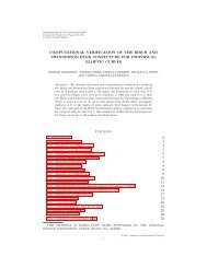
Even the simplest solution can be large (Watkins)
y 2 + y = x 3 − 5115523309x − 140826120488927
Numerator of x-coordinate of smallest solution (5454 digits):
Denominator:

The rank
The rank of E is essentially the number of independent
solutions.
◮ rank (E) = 0 means there are finitely many solutions.
◮ rank (E) > 0 means there are infinitely many solutions.
◮ The curve E(a) with equation
y(y + 1) = x(x − 1)(x + a)
has rank = 0, 1, 2, 3, 4 for a = 0, 1, 2, 4, 16.

The rank is finite
Can it be arbitrarily large?

The current record is rank(E) ≥ 28
y 2 + xy + y = x 3 − x 2 − 20067762415575526585033208209338542750930230312178956502x+
344816117950305564670329856903907203748559443593191803612660082962919394 48732243429

Peter Swinnerton-Dyer and Bryan Birch made a prediction for
the rank, based on the average number of solutions at prime
numbers p.

Primes
A prime p is a number greater than 1 that is not divisible by any
smaller number.
2, 3, 5, 7, 11, 13, 17, 19, 23, 29, 31, 37, 41, 43, 47, 53, 59, 61,
67, 71, 73, 79, 83, 89, 97, 101, 103, 107, 109, . . .
There are infinitely many primes. The largest explicit prime
known is 2 43112609 − 1 with 12,978,189 digits.
80
60
40
20
100 200 300 400 500

What do we mean by a solution of the cubic equation at the
prime number p?
y 2 + y = x 3 − x
(x, y) ≡ (3, 1) is a solution at p = 11
There are finitely many solutions A(p) at each prime p.
20
15
10
5
0
0 5 10 15 20
p =23, A(23) =22
70
60
50
40
30
20
10
0
0 10 20 30 40 50 60
p =71, A(71) =63
70

It is common to write
#{solutions mod p} = A(p) = p + 1 − a(p)
We define the L-function of E by the infinite product
L(E, s) =
all p
(1 − a(p)p −s + p 1−2s ) −1 = a(n)n −s
This definition only works in the region s > 3/2, where the
infinite product converges.
1
0.8
0.6
0.4
0.2
0
?
0 2 4 6 8

If we formally set s = 1 in the product, we get
all p
(1 − a(p)p −1 + p −1 ) −1 =
all p
p
A(p)
If A(p) is large on average compared with p, this will approach
0. The larger A(p) is on average, the faster it will tend to 0.
0.7
0.6
0.5
0.4
0.3
0.2
0.1
0
100 200 300 400 500

The conjecture of Birch and Swinnerton-Dyer
1. The function L(E, s) has a natural (analytic) continuation to
a neighborhood of s = 1.
2. The order of vanishing of L(E, s) at s = 1 is equal to the
rank of E.
3. The leading term in the Taylor expansion of L(E, s) at
s = 1 is given by certain arithmetic invariants of E.
L(E, s) = c(E)(s − 1) rank(E) + · · ·

The most mysterious arithmetic invariant was studied by John
Tate and Igor Shafarevich, who conjectured that it is finite. Tate
called this invariant X.

The Birch and Swinnerton-Dyer Conjecture
L(E, s) = c(E)(s − 1) rank(E) + · · ·
c(E) = ΩE · Reg E ·#XE · cp
#E(Q) 2 tor
Each quantity on the right measures the size of an
abelian group attached to E.

Natural (analytic) continuation
The infinite sum ∞
n=0 x n converges when −1 < x < 1.
1
1 − x =
∞
n=0
x n
-6 -5 -4 -3 -2 -1 1
7
6
5
4
3
2
1

Fermat’s Last Theorem
The natural (analytic) continuation of L(E, s) = a(n)n −s was
obtained (in most cases) by Andrew Wiles and Richard Taylor
(1995). They proved that the function defined by the infinite
series
is a modular form.
F(τ) = a(n)e 2πinτ

Combining a limit formula of Benedict Gross and Don Zagier
(1983) with work of Victor Kolyvagin (1986) we can now show
the following.
If L(E, 1) = 0 the rank is zero, so there are finitely many
solutions.
If L(E, 1) = 0 and L ′ (E, 1) = 0 the rank is one, so there are
infinitely many solutions.
In both cases, we can also show that X is finite.

Example: A Rank 1 Curve
sage: E = EllipticCurve([0,0,1,-1,0])
sage: L = E.lseries()
sage: Lser = L.taylor_series(); Lser
0.305999773834052*z + 0.186547797268162*zˆ2 + ...
sage: c = Lser[1]; c
0.305999773834052
sage: Omega_E = E.period_lattice().omega(); Omega_E
5.98691729246392
sage: Reg_E = E.regulator(); Reg_E
0.0511114082399688
sage: prod_cp = E.tamagawa_product_bsd(); prod_cp
1
sage: T = E.torsion_order()ˆ2; T
1
sage: c / (Omega_E * Reg_E * prod_cp / Tˆ2)
1.00000000000000

Example: A Rank 2 Curve
sage: E = EllipticCurve([0,1,1,-2,0])
sage: L = E.lseries()
sage: Lser = L.taylor_series(); Lser
-2.69e-23 + (1.52e-23)*z + 0.75931650028*zˆ2 + ...
sage: E.rank()
2
sage: c = Lser[2]
sage: Omega_E = E.period_lattice().omega()
sage: Reg_E = E.regulator()
sage: prod_cp = E.tamagawa_product_bsd()
sage: T = E.torsion_order()ˆ2
sage: c / (Omega_E * Reg_E * prod_cp / Tˆ2)
1.00000000000000
sage: S = E.sha(); S
Tate-Shafarevich group ...
sage: S.p_primary_bound(5)
0
Open Problem: Prove that X(E) is finite.

Example: A Rank 4 Curve
sage: E = EllipticCurve([0,15,1,-16,0])
sage: L = E.lseries()
sage: Lser = L.taylor_series(); Lser
4.32e-24 + (-1.96e-23)*z + (2.05e-22)*zˆ2
+ (-7.97e-22)*zˆ3 + 10.84*zˆ4 - ...
sage: E.rank()
4
sage: c = Lser[4]
sage: Omega_E = E.period_lattice().omega()
sage: Reg_E = E.regulator()
sage: prod_cp = E.tamagawa_product_bsd()
sage: T = E.torsion_order()ˆ2
sage: c / (Omega_E * Reg_E * prod_cp / Tˆ2)
0.99999999999999
Open Problem: Prove that ords=1 L(E, s) = 4.

Thank you