outdoor lighting and crime, part 1 - Astronomical Society of Victoria

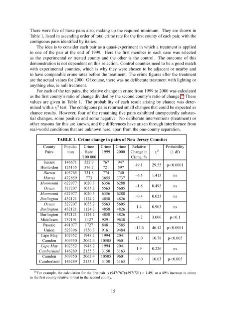
There were five of these pairs also, making up the required minimum. They are shown in
Table 1, listed in ascending order of total crime rate for the first county of each pair, with the
contiguous pairs identified by italics.
The idea is to consider each pair as a quasi-experiment in which a treatment is applied
to one of the pair at the end of 1999. Here the first member in each case was selected
as the experimental or treated county and the other is the control. The outcome of this
demonstration is not dependent on this selection. Control counties need to be a good match
with experimental counties, which is why they were chosen to be adjacent or nearby and
to have comparable crime rates before the treatment. The crime figures after the treatment
are the actual values for 2000. Of course, there was no deliberate treatment with lighting or
anything else, ie null treatment.
For each of the ten pairs, the relative change in crime from 1999 to 2000 was calculated
as the first county’s ratio of change divided by the second county’s ratio of change. 10 These
values are given in Table 1. The probability of each result arising by chance was determined
with a χ 2 test. The contiguous pairs returned small changes that could be expected as
chance results. However, four of the remaining five pairs exhibited unexpectedly substantial
changes, some positive and some negative. No deliberate interventions (treatment) or
other reasons for this are known, and the differences have arisen through interference from
real-world conditions that are unknown here, apart from the one-county separation.
TABLE 1. Crime change in pairs of New Jersey Counties
County Popula- Crime Crime Crime Relative Probability
Pairs tion Rate 1999 2000 Change in χ2 (1 df)
/100 000 Crime, %
Sussex
Hunterdon
146671
125135
522.9
576.2
767
721
947
597
49.1 29.55 p