Quantitative Example of Energy Compaction and Decorrelation

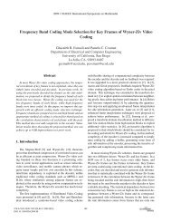
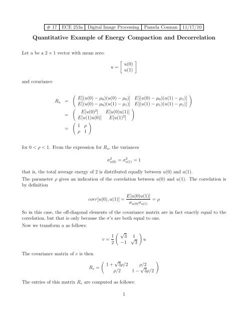
# 17 ECE 253a Digital Image Processing Pamela Cosman 11/17/10
Quantitative Example of Energy Compaction and Decorrelation
Let u be a 2 × 1 vector with mean zero:
and covariance
Ru =
=
=
u =
u(0)
u(1)
E[(u(0) − µ0)(u(0) − µ0)] E[(u(0) − µ0)(u(1) − µ1)]
E[(u(0) − µ0)(u(1) − µ1)] E[(u(1) − µ1)(u(1) − µ1)]
E[u(0) 2 ] E[u(0)u(1)]
E[u(1)u(0)] E[u(1) 2
]
1 ρ
ρ 1
for 0 < ρ < 1. From the expression for Ru, the variances
σ 2 u(0) = σ 2 u(1) = 1
that is, the total average energy of 2 is distributed equally between u(0) and u(1).
The parameter ρ gives an indication of the correlation between u(0) and u(1). The correlation is
by definition
corr[u(0), u(1)] = E[u(0)u(1)]
= ρ
σu(0)σu(1)
So in this case, the off-diagonal elements of the covariance matrix are in fact exactly equal to the
correlation, but that is only because the σ’s are both equal to one.
Now we transform u as follows:
The covariance matrix of v is then
Rv =
v = 1
√
3 1
2 −1 √ 3
u
1 + √ 3ρ/2 ρ/2
ρ/2 1 − √ 3ρ/2
The entries of this matrix Rv are computed as follows:
1

√
3 1
v(0) = u(0) +
2 2 u(1)
E[v(0) 2 ] = 3
√
1 3
+ + 2
4 4 4 ρ
etc. Now if we compare the energy of the two coordinates:
σ 2 v(0) = 1 + √ 3ρ/2
σ 2 v(1) = 1 − √ 3ρ/2
we see that the total average energy is still 2, but now the energy in v(0) is greater than in v(1). If
ρ = 0.95, then 91.1% of the total average energy has been packed in the first sample.
σ 2 v(0) = 1.82 σ2 v(1)
The correlation between v(0) and v(1) is given by
ρv(0,1) = E[v(0)v(1)]
=
σv(0)σv(1)
ρ
= 0.18
2
(1 − 3
4 ρ2 )
which is less in absolute value than | ρ | for | ρ |< 1 For ρ = 0.95, we find ρv(0,1) = 0.83. Hence the
correlation between the transform coefficients has been reduced.
Suppose instead we use the transform matrix
then we find
A = 1 √ 2
σ 2 v(0)
σ 2 v(1)
1 1
1 −1
= 1 + ρ
= 1 − ρ
ρv(0,1) = 0
For ρ = 0.95, now 97.5% of the energy is packed into v(0), and the two components v(0) and v(1)
are uncorrelated.
2

DCT basis images for 8x8 blocks:
Luminance Quantization Table:
16 11 10 16 24 40 51 61
12 12 14 19 26 58 60 55
14 13 16 24 40 57 69 56
14 17 22 29 51 87 80 62
18 22 37 56 68 109 103 77
24 35 55 64 81 104 113 92
49 64 78 87 103 121 120 101
72 92 95 98 112 100 103 99
Chrominance Quantization Table:
17 18 24 47 99 99 99 99
18 21 26 66 99 99 99 99
24 26 56 99 99 99 99 99
47 66 99 99 99 99 99 99
99 99 99 99 99 99 99 99
99 99 99 99 99 99 99 99
99 99 99 99 99 99 99 99
99 99 99 99 99 99 99 99
3