Computing with diode model

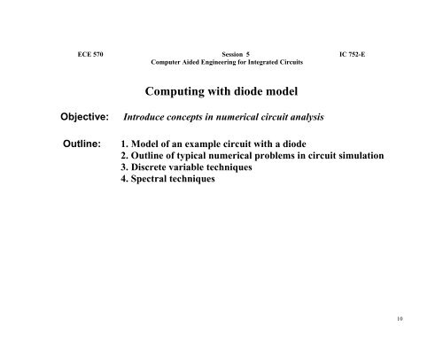
ECE 570 Session 5 IC 752-E
Computer Aided Engineering for Integrated Circuits
Computing with diode model
Objective: Introduce concepts in numerical circuit analysis
Outline: 1. Model of an example circuit with a diode
2. Outline of typical numerical problems in circuit simulation
3. Discrete variable techniques
4. Spectral techniques
10

1. Model of an example circuit with a diode
We shall examine a simple diode configuration (a simplistic model of half-way rectifier) on the left
and its equivalent circuit on the right.
+ r - E G
+
-
The resistor r in the equivalent circuit represents the internal resistance, r G , of the source and the
diode resistance r s . For simplicity we assume that Q D represent the diode junction charge
storage.
The equation for the diode voltage v written using the equivalent circuit is
v
dv nV E − v
T
c( v) = = − − I s e − − 1 +
+
E
dt r
r
+
v
-
i
D
QD
11

c v
dQ
dv
where ( ) D
P-N junction diode model.
= is the incremental junction capacitance defined in the section describing the
12

2. Outline of typical numerical procedures in simulation of a circuit.
D-C analysis
Steady state solution of circuit equations with all derivatives equated to zero.
In the circuit this means that capacitors are open and inductors shorted.
In the example circuit the D-C analysis is defined by the nonlinear algebraic equation
0 = = − −I s
v
nVT
e − − 1
e − v
+
+
This equation is solved via linear approximation and iterations (N-R).
D-C analysis is basic for other analyses (A-C, transient, distortion) as it determines IC’s & OP’s.
Transient analysis
Often used, very involved, expensive in CPU time.
Discrete variable techniques
Variables are computed in discrete times.
r
Spectral techniques
Series expansion of circuit variables
13

3. Discrete variable techniques (time marching methods)
Basic methods (must be implicit): single step [Backward Euler (B-E), trapezoidal (TR)]
multistep [Gear’s].
Procedures
1.Time discretization.
The circuit variables are computed in the discrete times t [ t0 , t1, t2 ,..., tM
]
∈ .
Example of circuit equation in discrete variables (diode circuit discretized using B-E)
( )
v
k+
1
v − − v nV E −
− v
T
c v = = − − I e − − 1 +
+
k + + 1 k k + + 1 k +
+
1
k + 1
tk + 1 − tk s
r
k =
0,1,2,3,... M
14

where k v is the numerical approximation to v( tk
). The initial condition (starting
point), o v , is usually defined through D-C analysis. The equation is implicit because the
unknown, k v + 1 , has to be computed from the non-linear equation. The difference,
t t
k + 1 k − , is the numerical integration step size.
3.1. Linearization.
v y
To simplify the notation we shall designate k + 1 = , and thus consider the problem of finding
a solution for one step only ( k + 1 ). With this notation the circuit equation becomes
y − − v
( ) k c y
tk + 1 − tk = = − −I s
y
nVT
e − − 1
Ek + 1 −
−
y
+
+
. r
The nonlinear elements are linearized using Taylor expansion around a temporary operating point ,
(starting point) y , and resulting linear network is solved to determine the improved value, y + 1 .
15

It should be pointed here that in the linearization procedure we consider only first two terms of the
expansion so a single solution of the resulting equations may not be adequate and iterations are
usually required.
3.2. Linearization of VCCS in the diode model.
To illustrate the procedure we apply the linearization to the current source (VCCS) of the example
diode circuit. The resulting relation in the iterative form with the iteration count, , is
or else
y y
I
= = − − 1 + + + 1 −
−
nV
( )
nVT s nVT
i I e e y y
D s
y y y
I I
= = − − 1 − − +
+
+
nVT s nVT s nVT
i I e e v e y
D s k
nVT nVT
I
D
T
G
D
1
.
16

This right hand side of this relation is used to replace the VCCS equation and shows that the
linearization can be interpreted as a replacement of the original nonlinear VCCS by an independent,
constant current source, I D , defined by
I D = = I s
y
nVT e − − 1
I s −
−
nVT
y
nVT
e vk
and connected in parallel with the conductance, G D , which is also a constant
GD I s =
nVT
y
nVT
e
of the value determined by the known voltage, y , (known as a starting point or as a result of
previous iteration).
The circuit interpretation of VCCS linearization is illustrated on the next page.
17

The linearized circuit representation of VCCS
+
v
-
D
+
v D
-
+
-
+
y + 1
3.3. Linearization of capacitor relations in the diode model.
iD
linear
equivalent
To discuss the capacitor linearization procedure is convenient to rewrite the discretized circuit
equation in the form
y
( ) ( )
nV E T
k + 1 y
g y y g y vk I s e 1 −
− − = = − − − − +
+
-
GD
I Dl
r
18

where
( )
g y
=
( )
c y
t − t
k + 1 k
represents the nonlinear conductance.
The linearization of capacitor is performed replacing the nonlinear relation
dg
g( y + + 1) = = g( y ) + + ( y +
+
1 − − y ) .
dy
y= y
g ( y ) by
Applying this expansion to the left side of the discretized circuit equation and retaining constant and
linear terms only we obtain
y
nV E T
k + 1 − y
− − Ic + + Gc y + 1 = = − −I s e − − 1 +
+
where the equivalent current source, c I , and conductance, c G , are defined by the following
relations:
r
19

and
dg
I ( ) ( )
c = = g y vk + + y −
− vk y
dy
y= y
dg
G = = g y + + y −
−
v
dy
( ) ( )
c k
y= y
.
20

These linearization procedures can be interpreted in terms of an equivalent circuit
+
v D
linear
c c G y + 1
equivalent
circuit
which is composed of conductance, c G , and current source, c I . The conductance and current
source values are updated at each iteration.
+
-
I c
21

3.4. The linearized equivalent circuit of the example circuit with a junction diode.
Using the linearized VCCS and capacitor circuits we can finally construct the equivalent linear
circuit for the introduced here example of nonlinear network with a diode. Such a network is used in
the circuit iterative solution procedure and is often called companion network.
+
-
r
Ek + 1
+
y + 1
-
G D
It should be emphasized here that all elements of equivalent circuit (companion network) are
constant - the circuit model is in the form of linear algebraic equations. However, the coefficients are
updated from iteration to iteration.
I Dl
Gc
I
c
22

4. Spectral techniques
Linearization in the case of spectral techniques is based on Newton-Kantorovich approach and
results in a linear circuit with time varying coefficients. The equivalent linear network has time
varying elements which is very distinct from the result of linearization used in conjunction with time
marching methods where all elements are fixed. The circuit model is in the form of linear differential
equations with time varying coefficients.
This major distinction stems from the fact that the linearization is performed not around a fixed
v = v t ) evolving in time.
operating point ( y ), but around a trajectory, ( ( )
4.1. Linearization of capacitor relations.
p p
The linearization of left side of the circuit equation (involving the linearization of capacitor)
dv
( )
nV E − v
T
c v = = − − I s e − − 1 +
+
dt r
v
23

equires an additional explanation. It should be noted that v and
such that he left side is interpreted as a function of two variables ( )
dv
z
dt = are treated independently
y z
ϕϕϕϕ , .
A linear expansion of a function with two arguments around, ( y p, z p ), can be obtained as follows
∂∂ ∂∂ ϕϕ ϕϕ ∂∂ ∂∂ ϕϕ
ϕϕ
ϕϕ ϕϕ + + Δ Δ + + Δ Δ = = ϕϕ
ϕϕ
+ + Δ Δ + + Δ
Δ
( y , z ) ( y , z )
p y p z p p y z
∂∂ ∂∂ y y ∂∂
∂∂
z y
p p
z z
p p
The function, ϕϕϕϕ ( y, z)
, in the case of interest has a very simple form ( )
arguments is
( ) ( ) ( ) ( )
p v p z
( ) + + Δ
Δ ( )
c y z , which showing all
dv
d v
( ) ( ) ( )
p t v t
c v = = c v p t + + Δ Δ v t
=
=
dt dt
= = c v t + + Δ Δ t z t + + Δ
Δ
t
.
24

Expanding this function according to the discussed rule and arranging the terms we obtain
the following linear approximation
dv
c( v) ≈
dt
≈ ≈ c v p ( t) dv ( t) dc
+ +
dt dv
dv p ( t) dc
v ( t) −
−
dt dv
dv p t
v p ( t)
dt
( )
We shall introduce the time varying conductance
and the time varying current source
v t v t
p p
( )
G t
cp
( )
G I
cp cp
=
dc
p
( )
v t
p
( )
dv t
dv dt
( )
.
25

where v = v p + Δ v
p
( )
v t
( )
dc dv
( ) ( )
p t
Icp t = v p t
dv dt
or else showing the independent variable explicitly
( ) ( ) ( )
v t = v t + Δ v t .
p
.
26

Using the introduced notation for the given functions we can write the linearized relation in a
compact form
( )
dv
dv t
c( v) ≈ ≈ c v ( ) p t + + Gcp t v t −
− Icp t
dt dt
( ) ( ) ( )
which in the circuit interpretation means that the equivalent circuit for the nonlinear capacitor is a
parallel connection of time varying capacitance, conductance, and current source:
+
v
-
linear
c G ( t)
equivalent circuit
(time varying
elements)
+
v t
( )
-
cp
cp
( )
I t
( )
c v t
p
27

4.2. Linearization of I-V characteristic.
The linearization of the right side of the circuit equation is straightforward and yields
( )
dv t
c v ( )
( ) ( ) ( )
p t + + Gcp t v t − − Icp t =
=
dt
( ) ( )
v t v t v t
p p p
nV I
( )
( )
T s nV I
T s nV E−v t
T
=− =−I e − − 1 + + e v t − − e v t +
+
nV nV r
.
s p
T T
I
Dp
G
Dp
( )
( )
28

Introducing the time dependent current source defined by the formula
( )
( ) ( )
v t v t
p p
I t I
nVT e 1 s nVT
e v t
= = − − −
−
Dp s p
nVT
and time dependent conductance defined as
( )
I
p
( )
v t
s nV
GD t e
p nVT
we can write the linearized circuit equation in the following compact form
=
I
T
( )
29

( )
c v ( ) p t
dv t
dt
+ + G ( ) ( ) ( )
cp t v t − − Icp t =
=
E−v( t)
=− =− I ( ) ( ) ( )
Dp t − − GD t v t +
+
p r
which forms a linear differential equation with time varying coefficients.
30

4.3. Linearized equivalent circuit of diode network.
The linearized dynamic circuit for simulation of diode network using spectral techniques is shown in
the schematics below. The circuit is dynamic as it contains the capacitor, c v p ( t ) . To solve the
circuit a waveform, v p ( t ) , needs to be supplied to determine all time dependent circuit
components.
+
- E r
+
( )
v t
-
Dp
( )
G t
Dp
( )
I t
( )
G t
cp
( )
I t
cp
( )
c v t
p
31