Rational functions - Cs.ioc.ee

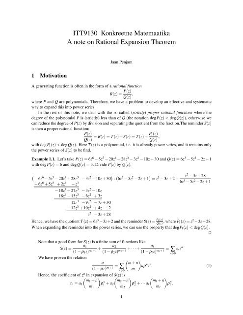
1 Motivation
ITT9130 Konkreetne Matemaatika
A note on Rational Expansion Theorem
Jaan Penjam
A generating function is often in the form of a rational function
R(z) = P(z)
Q(z) ,
where P and Q are polynomials. Therefore, we have a problem to develop an effective and systematic
way to expand this into power series.
In the rest of this note, we deal with the so called (strictly) proper rational functions where the
degree of the polynomial P is (strictly) less than of Q (the notation degP(z) < degQ(z)), otherwise we
can reduce the degree of P(z) by division and separating the quotient from the fraction.The reminder S(z)
is then a proper rational function:
P(z)
Q(z)
with degP1(z) < degQ(z). Here T (z) is a polynomial, i.e. it is already power series, and it remains only
the power series of S(z) to be find.
= R(z) = T (z) + S(z) = T (z) + P1(z)
Q(z) ,
Example 1.1. Let’s take P(z) = 6z 6 − 5z 5 − 20z 4 + 28z 3 − 3z 2 − 10z + 30 and Q(z) = 6z 3 − 5z 2 − 2z + 1
with degP(z) = 6 and degQ(z) = 3. Divide P(z) by Q(z):
6z6 − 5z5 − 20z4 + 28z3 − 3z2 − 10z + 30 : 6z3 − 5z2 − 2z + 1 = z3 − 3z + 2 + z2 − 3z + 28
6z3 − 5z2 − 2z + 1
− 6z6 + 5z5 + 2z4 − z3 − 18z 4 + 27z 3 − 3z 2 − 10z
18z 4 − 15z 3 − 6z 2 + 3z
12z 3 − 9z 2 − 7z + 30
− 12z 3 + 10z 2 + 4z − 2
z 2 − 3z + 28
Hence, we have the quotient T (z) = 6z 3 −3z+2 and the reminder S(z) = P1(z)
Q(z) , where P1(z) = z 2 −3z+28.
When expanding the reminder into the power series, we can use the property that degP1(z) < degQ(z).
✷
Note that a good form for S(z) is a finite sum of functions like
a1
a2
S(z) =
+
+ ··· +
(1 − ρ1z) m1+1 (1 − ρ2z) m2+1
We have proven the relation
m1
a
(1 − ρz) m+1 = ∑ n0
m2
m + n
m
aℓ
(1 − ρℓz) mℓ+1 = ∑ snz
n0
n
aρ n z n
Hence, the coefficient of zn
in expansion
of S(z) is
m1 + n
sn = a1 ρ n
m2 + n
1 + a2 ρ n
mℓ + n
2 + ···aℓ ρ n ℓ .
1
mℓ
(1)

Rational Expansion Theorem Jaan Penjam
In particular, when m1 = m2 = ... = mℓ = 0, the latter formula takes the form
. (2)
2 Reflected polynomials
Let
sn = a1ρ n 1 + a2ρ n 2 + ··· + aℓρ n ℓ
Q(z) = aℓz ℓ + aℓ−1z ℓ−1 + ··· + a2z 2 + a1z + a0
is a polynomial over the field of complex numbers C. Then the polynomial
Q R (z) = a0z ℓ + a1z ℓ−1 + ··· + aℓ−2z 2 + aℓ−1z + aℓ
is called its reflected polynomial.
Property 2.1. If ρ1,...,ρℓ are roots of the polynomial Q R ( 1
z ), then Q(z) = (1 − ρ1z)···(1 − ρℓz).
Proof. Having ρ1,...,ρℓ as roots of the reflected polynomial means that QR ( 1 1
1
z ) = a0( z −ρ1)···( z −ρℓ).
On theother hand,
Hence,
Q(z) = aℓz ℓ + aℓ−1z ℓ−1 + ··· + a2z 2 + a1z + a0 =
= z ℓ
= z ℓ Q R
aℓ + aℓ−1
1
z
Q(z) = z ℓ Q R
= z ℓ a0
1 1
+ ··· + a2
z z
ℓ−2 + a1
1
z
ℓ−1 + a0
1
=
z
1 1
− ρ1 ··· − ρℓ =
z z
= z ℓ 1 − zρ1 1 − zρℓ
a0 ··· =
z z
= a0(1 − zρ1)···(1 − zρℓ)
1
zℓ
=
Example 2.1. The polynomial Q(z) = 6z 3 − 5z 2 − 2z + 1 from Example 1.1 has the following reflected
polynomial
Q R (z) = z 3 − 2z 2 − 5z + 6 =
= z 3 − (z 2 + z 2 ) + (z − 6z) + 6 =
= z 2 (z − 1) − z(z + 1) − 6(z − 1) =
= (z − 1)(z 2 − z − 6) =
= (z − 1)(z 2 + 2z − 3z − 6) =
= (z − 1)(z(z + 2) − 3(z + 2)) =
= (z − 1)(z + 2)(z − 3)
2

Rational Expansion Theorem Jaan Penjam
This says us that Q R (z) has the roots 1, −2 and 3 and due to Proposition 1.1 the following factorization
of Q(z) is valid:
Q(z) = (1 − z)(1 + 2z)(1 − 3z).
Let’s check this result, that is compute the last formula by opening the parenthesis.
(1 − z)(1 + 2z)(1 − 3z) = (1 + z − 2z 2 )(1 − 3z) =
3 Decomposition into partial fractions
= 1 + z − 2z 2 − 3z − 3z 2 + 6z 3 =
= 6z 3 − 5z 2 − 2z + 1 = Q(z)
If all roots of the QR (z) are distinct and the denominator of the fraction P(z)
Q(z) is factorizable as Q(z) =
a0(1 − zρ1)···(1 − zρℓ), we may expect that the fraction can be written as
P(z) A1 A2
Aℓ
= + + ··· + . (3)
Q(z)
1 − ρ1z
1 − ρ1z
1 − ρℓz
If degP(z) < degQ(z) = ℓ, then the equation (3) determines the system of linear equations for finding
constants A1,A2,...,Aℓ. We demonstrate this in the following example.
Example 3.1. Let’s factorize the fraction S(z) = P1(z)
Q(z) from Example 1.1. We have P1(z) = z 2 − 3z + 28
and Q(z) = (z − 1)(z + 2)(z − 3). Hence,
P1(z)
Q(z)
A B C
= + +
1 − z 1 + 2z 1 − 3z =
= A(1 + 2z)(1 − 3z) + B(1 − z)(1 − 3z) +C(1 − z)(1 + 2z)
Q(z)
= A(1 − z − 6z2 ) + B(1 − 4z + 3z 2 ) +C(1 + z − 2z 2 )
Q(z)
= (−6A + 3B − 2C)z2 + (−A − 4B +C)z + (A + B +C)
Q(z)
Comparing the numerator of this fraction
⎧
with the polynomial P1(z) leads to the system of equations:
⎨−6A
+ 3B − 2C = 1
−A − 4B +C
⎩
A + B +C
= −3
= 28
We start solving of this system by computing
the determinant
−6
3 −2
D =
−1
−4 1
= 30.
1 1 1
Then we can find the solution
1 3 −2
−3
−4 1
28 1 1
A =
= −
D
13
3
−6
−1
1
B =
1
−3
28
D
−2
1
1
= 119
15
−6
−1
1
C =
3
−4
1
D
1
−3
28
= 122
5 .
3
=
=
✷

Rational Expansion Theorem Jaan Penjam
So, we have
S(z) = −13
3(1 − z) +
119 122
+
15(1 + 2z) 5(1 − 3z) .
All roots of Q(z) are distinct, so the equation (2) is applicable and the power series S(z) = ∑n0 snzn ,
where the coefficient
sn = − 13 119
+
3 15 (−2)n + 122
5 3n .
✷
4 Rational Expansion Theorem
The method of partial fractions may produce huge systems of equations to be solved. The following
theorem gives an alternative technique to mess around the problem.
Theorem 4.1. (for Distinct Roots) If R(z) = P(z)/Q(z) the generating function for the sequence 〈rn〉,
where Q(z) = (1 − ρ1z)(1 − ρ2z)···(1 − ρℓz) and the numbers (ρ1,...,ρℓ) are distinct,
and if P(z) is a polynomial of degree less than ℓ, then
rn = a1ρ n 1 + a2ρ n 2 + ··· + aℓρ n ℓ , where ak = −ρkP(1/ρk)
Q ′ .
(1/ρk)
Proof. Construct the sum
S(z) = a1
aℓ
+ ··· +
1 − ρ1z 1 − ρℓz ,
where the constants ak are as defined in the theorem. We show that T(z)=R(z)-S(z)=0. For that reason, it
is sufficient (cf. properties of rational functions, for example in http://en.wikipedia.org/wiki/Rational_function)
to confirm that limz→∞ T (z) = 0 and that T (z) is never infinite.
Satisfiability of the first condition follows from the observation that both limz→∞ R(z) = 0 and limz→∞ S(z) =
0, because of degrees of numerators is less than degree of corresponding denominators.
Only the points where T (z) may approach to infinity are 1/ρk. Hence, to show that limz→αk T (z) = ∞,
were αk = 1/ρk, it suffers to prove that
lim (z − αk)R(z) = lim (z − αk)S(z).
z→αk
z→αk
Due to
ak(z − αk)
1 − ρ jz = ak(z − 1
ρk )
1 − ρ jz = −ak(1 − ρkz)
→ 0, if k = j and z → αk.
ρk(1 − ρ jz)
The right-hand side of this assertion is
lim
z→αk
(z − αk)S(z) = lim (z − αk)
z→αk
ak(z − αk)
1 − ρkz
= −ak
ρk
= P(1/ρk)
Q ′ (1/ρk)
The left-hand limit can be transformed due to L’Hospital’s Rule (see in more details on
http://mathworld.wolfram.com/LHospitalsRule.html) as follows
lim (z − αk)R(z) = lim (z − αk)
z→αk
z→αk
P(z)
Q(z) = P(αk)
z − αk
lim
z→αk Q(z)
P(αk)
=
Q ′ P(1/ρk)
=
(αk) Q ′ (1/ρk)
Example 4.1. Consider the fraction S(z) = P1(z)
Q(z) from Example 1.1 once more. To use theorem 4.1, we
shall compute values P1( 1/ρ) and Q( 1/ρ) for ρ = ρ1,ρ2,ρ3 first.
We have P1(z) = z2 − 3z + 28. Hence,
1
P1 =
ρ
1 3 1 − 3ρ + 28ρ2
− + 28 =
ρ2 ρ ρ2 4

Rational Expansion Theorem Jaan Penjam
and thus we get for ρ1 = 1,ρ2 = −2,ρ3 = 3:
So,
1 1
P1 = P1 =
ρ1 1
1 − 3 + 28
= 26
1
1 1
P1 = P1 =
ρ2 −2
1 + 6 + 28 · 4
=
4
119
4
1 1
P1 = P1 =
ρ3 3
1 − 9 + 28 · 9
=
9
244
9
On the another hand, Q(z) = (z − 1)(z + 2)(z − 3) = 6z3 − 5z2 − 2z + 1 gives Q ′ (z) = 18z2 − 10z − 2.
Q
that provides the following values
1
ρ
= 18 10
−
ρ2 ρ
18 − 10ρ − 2ρ2
− 2 =
ρ2 ,
Q ′
1
= Q
ρ1
′
1
=
1
18 − 10 − 2
= 6
1
Q ′
1
= Q
ρ2
′
1
=
−2
18 + 10 · 2 − 2 · 4
=
4
15
2
Q ′
1
= Q
ρ3
′
1
=
3
18 − 10 · 3 − 2 · 9
= −
9
10
3
Finally we can compute the coefficients defined in the Theorem 4.1:
a1 = −ρ1P1(1/ρ1)
Q ′ −1 · 26
= = −13
(1/ρ1) 6 3
a2 = −ρ2P1(1/ρ2)
Q ′ (1/ρ2)
= 2 · 119 · 2
4 · 15
= 119
15
a3 = −ρ3P1(1/ρ3)
Q ′ −3 · 244 · 3
= = −122
(1/ρ3) 9 · (−10) 5
and write down the power series we are looking for: S(z) = ∑n0 snzn , where the coefficient
sn = − 13 119
+
3 15 (−2)n + 122
5 3n .
5 General expansion theorem for rational generating functions
Theorem 5.1. (for possibly Multiple Roots) If R(z) = P(z)/Q(z) the generating function for the sequence
〈rn〉, where Q(z) = (1 − ρ1z) d1 ···(1 − ρℓz) dℓ and the numbers (ρ1,...,ρℓ) are distinct,
and if P(z) is a polynomial of degree less than d1 + ... + dℓ, then
rn = f1(n)ρ n 1 + ··· + fℓ(n)ρ n ℓ , for all n 0,
where each fk(n) is a polynomial of degree dk − 1 with a leading coefficient
(−ρk) dkP(1/ρk)dk
ak =
Q (dk)
P(1/ρk)
=
(1/ρk) (dk − 1)!∏j=k(1 − ρ j/ρk) d j
This can be proved by induction on max(d1,...,dℓ), using the fact that
R(z) − a1(d1 − 1)!
(1 − ρ1z) d1 − ··· − aℓ(dℓ − 1)!
(1 − ρℓz) dℓ
5
✷

Rational Expansion Theorem Jaan Penjam
is a rational function whose denominator polynomial is not divisible by (1 − ρkz) dk for any k.
6 Decomposition into of partial fractions for multiple roots
Let R(z) = P(z)/Q(z) to be a strict proper rational function. If Q R (z) has a multiple root ρ, say, having
multiplicity k, then the formula of partial fractions of R(z) contains the following terms related to ρ:
Ai1
1 − ρz +
Ai2
+ ··· +
(1 − ρz) 2 Aik
,
(1 − ρz) k
where Ai1 ,Ai2 ,...,Aik are constants. The power series of these terms is defined by the equation (1).
Example 6.1. Let
Then
and
The partial fraction expansion can be written as
R(z) = A
1 − 2z +
R(z) = P(z)
Q(z) =
z − 1
−40z4 + 52z3 − 18z2 − z + 1 .
Q R (z) = z 4 − z 3 − 18z 2 + 52z − 40 = (z − 2) 3 (z + 5)
B
+
(1 − 2z) 2
Q(z) = (1 − 2z) 3 (1 + 5z).
C D
+
(1 − 2z) 3 1 + 5z =
= A(1 − 2z)2 (1 + 5z) + B(1 − 2z)(1 + 5z) +C(1 + 5z) + D(1 − 2z) 3
(1 − 2z) 3 (1 + 5z)
= A(5z3 − 16z 2 + z + 1) + B(−10z 2 + 5z + 1) +C(1 + 5z) + D(−8z 3 + 12z 2 − 6z + 1)
Q(z)
= (5A − 8D)z3 + (−16A − 10B + 12D)z2 + (A + 5B + 5C − 6D)z + (A + B +C + D)
Q(z)
Due to P(z), the constants A,B,C and D satisfy the equations:
⎧
⎪⎨
5A − 8D = 0
−16A − 10B + 12D = 0
⎪⎩
A + 5B + 5C − 6D
A + B +C + D
= 1
= −1
This system of equations has the solution: A = −16/29,B = 68/145,C = −83/145,D = −10/29. Using equality 1 we obtain
16
R(z) = −
29(1 − 2z) +
68
83 10
−
−
145(1 − 2z) 2 145(1 − 2z) 3 29(1 + 5z) =
0 + n 16
0
1 + n 68
1
2 − n 83
2
0 + n 10
0 29 3nz n =
= − ∑ n0
29 2n z n + ∑ n0
= − 1
145 ∑
80 − 68(n + 1) −
n0
145 2n z n − ∑ n0
83(n + 1)(n + 2)
2
2
n + 50 · 3 n
z n =
= − 1
145 ∑ 2 n−1 n
83n − 113n + 190 2 + 50 · 3
n0
z n
6
=
145 2n z n + ∑ n0
=
✷

Rational Expansion Theorem Jaan Penjam
7 Complex numbers vs real numbers
Everything above is valid for the polynomials over complex fields, i.e. all variables and coefficients are
complex numbers. The methods described work also for real numbers, but only if the polynomial Q(z)
has ℓ real roots, where degQ(z) = ℓ. The assumption that a polynomial has as many roots as its degree is
guaranteed for complex numbers by the Fundamental Theorem of Algebra. This is the reason why you
are strongly suggested to apply complex analysis in this context.
However, it is possible to keep yourself to real numbers as well, but you need to consider possibly
much more complex calculations. For example, to decompose a rational function into partial fractions
within real numbers, you have to consider, that a real polynomial Q(x) can have two types of irreducible
factors:
• x − ρ, where ρ is a real root of Q(x);
• x 2 + px + q, where p and q are real numbers such that p 2 < 4q.
Factors of both types can appear multiple times in the polynomial. Recall the techniques of such decomposition
in notes of your undergraduate course of mathematical analysis, for example pages 111–118 in
http://staff.ttu.ee/~janno/ma1chem.pdf.
To use method of Decomposition into Partial Fractions parts of the rational function R(x) = P(x)/Q(x)
are of the form
•
A1 A2
x−ρ + (x−ρ) 2 + ··· + Ak
(x−ρ) k , for a root ρ ∈ R with multiplicity k;
• B1+C1x
x2 B2+C2x
+ +px+q (x2 +px+q) 2 + ··· + Bk+Ckx
(x2 +px+q) k for a factor x2 + px + q with multiplicity k.
All constants Ai,Bi,Ci should be found by solving the system of linear equations similarly to case of
complex numbers (see Example 6.1).
After decomposition, parts of the form A1
x−ρ can be transformed into the poewer series similarly to
the formula 2:
1
n + k − 1 xk =
(x − ρ) k k − 1 ρk 1
(−ρ) k (1 − 1
ρ x)k = (−1)k · 1
ρ k ∑ n0
Unfortunately, in general, the parts of the form B+Cx
x 2 +px+q
does not have a simple transformation into
power series. For particular numbers p and q the assistance of an one-line Taylor Series Calculator
may be helpful. See for example, the Wolfram|Alpha Widgets on http://www.wolframalpha.com/
widgets/view.jsp?id=f9476968629e1163bd4a3ba839d60925. Some first terms of decomposition
of the fraction 1/(x 2 + px + q) looks like:
1
x2 1 px
= −
+ px + q q q2 + (p2 − q)x2 q3 − (p3 − 2pq)x3 q4 mmmmmmmmmmmmmmmmmmmjj − (p5 − 4p 3 q + 3pq 2 )x 5
7
q 6
+ (p4 − 3p2q + q2 )x4 q5 −
+ (p6 − 5p 4 q + 6p 2 q 2 − q 3 )x 6
q 7
− ···