Perturbation theory, bands, and the Dirac equation - Faculty.virginia ...
Perturbation theory, bands, and the Dirac equation - Faculty.virginia ...
Perturbation theory, bands, and the Dirac equation - Faculty.virginia ...

You also want an ePaper? Increase the reach of your titles
YUMPU automatically turns print PDFs into web optimized ePapers that Google loves.
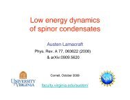
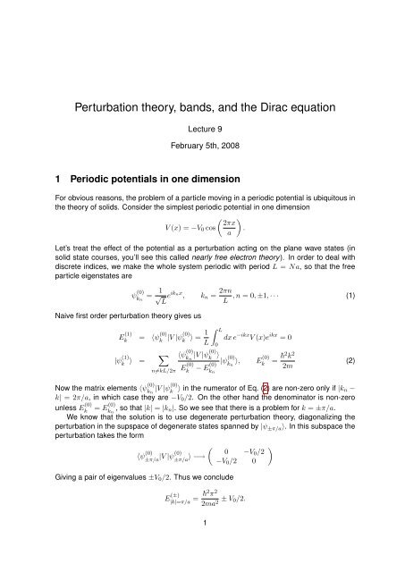
<strong>Perturbation</strong> <strong><strong>the</strong>ory</strong>, <strong>b<strong>and</strong>s</strong>, <strong>and</strong> <strong>the</strong> <strong>Dirac</strong> <strong>equation</strong><br />
Lecture 9<br />
February 5th, 2008<br />
1 Periodic potentials in one dimension<br />
For obvious reasons, <strong>the</strong> problem of a particle moving in a periodic potential is ubiquitous in<br />
<strong>the</strong> <strong><strong>the</strong>ory</strong> of solids. Consider <strong>the</strong> simplest periodic potential in one dimension<br />
<br />
2πx<br />
V (x) = −V0 cos .<br />
a<br />
Let’s treat <strong>the</strong> effect of <strong>the</strong> potential as a perturbation acting on <strong>the</strong> plane wave states (in<br />
solid state courses, you’ll see this called nearly free electron <strong><strong>the</strong>ory</strong>). In order to deal with<br />
discrete indices, we make <strong>the</strong> whole system periodic with period L = Na, so that <strong>the</strong> free<br />
particle eigenstates are<br />
ψ (0)<br />
kn<br />
= 1<br />
√ L e iknx , kn = 2πn<br />
Naive first order perturbation <strong><strong>the</strong>ory</strong> gives us<br />
E (1)<br />
k = 〈ψ (0)<br />
k<br />
|ψ (1)<br />
k 〉 =<br />
<br />
n=kL/2π<br />
Now <strong>the</strong> matrix elements 〈ψ (0)<br />
kn<br />
k<br />
1<br />
|V |ψ(0)<br />
k 〉 =<br />
L<br />
L<br />
0<br />
〈ψ (0)<br />
|V |ψ(0)<br />
kn<br />
E (0)<br />
k<br />
k 〉<br />
− E(0)<br />
kn<br />
L<br />
, n = 0, ±1, · · · (1)<br />
dx e −ikx V (x)e ikx = 0<br />
|ψ (0)<br />
〉, E(0)<br />
kn k = 2k2 2m<br />
|V |ψ(0)<br />
k 〉 in <strong>the</strong> numerator of Eq. (2) are non-zero only if |kn −<br />
k| = 2π/a, in which case <strong>the</strong>y are −V0/2. On <strong>the</strong> o<strong>the</strong>r h<strong>and</strong> <strong>the</strong> denominator is non-zero<br />
unless E (0)<br />
= E(0)<br />
kn , so that |k| = |kn|. So we see that <strong>the</strong>re is a problem for k = ±π/a.<br />
We know that <strong>the</strong> solution is to use degenerate perturbation <strong><strong>the</strong>ory</strong>, diagonalizing <strong>the</strong><br />
perturbation in <strong>the</strong> supspace of degenerate states spanned by |ψ ±π/a〉. In this subspace <strong>the</strong><br />
perturbation takes <strong>the</strong> form<br />
〈ψ (0)<br />
±π/a |V |ψ(0)<br />
±π/a 〉 −→<br />
Giving a pair of eigenvalues ±V0/2. Thus we conclude<br />
E (±)<br />
<br />
|k|=π/a = 2 π 2<br />
0 −V0/2<br />
−V0/2 0<br />
± V0/2.<br />
2ma2 1<br />
<br />
(2)
E (±) (k)<br />
14<br />
12<br />
10<br />
8<br />
6<br />
4<br />
2<br />
0 1 2 3 4 5 6<br />
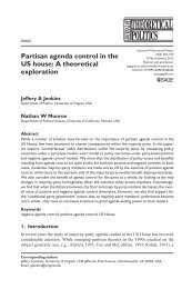
Figure 1: Dispersions relations E (±) (k) from degenerate perturbation <strong><strong>the</strong>ory</strong> along with <strong>the</strong><br />
unperturbed eigenvalues.<br />
Of course, as we approach <strong>the</strong> points k = ±π/a <strong>the</strong> denominators in <strong>the</strong> nonvanishing terms<br />
in Eq. (2) become large, so it makes sense to treat those nearby k values in <strong>the</strong> same way.<br />
In <strong>the</strong> 2 × 2 subspace spanned by k <strong>and</strong> k − 2π/a, we <strong>the</strong>n have <strong>the</strong> matrix elements of <strong>the</strong><br />
total Hamiltonian <br />
εk −V0/2<br />
,<br />
−V0/2 εk−2π/a with eigenvalues (∆k = k − π/a)<br />
E (±)<br />
k<br />
= 2 π 2<br />
2ma 2 + 2 ∆k 2<br />
2m ±<br />
2 ∆kπ<br />
ma<br />
2<br />
+<br />
2 V0<br />
2<br />
The eigenvalues are sketched in Fig. 1 . A few comments are worth making at this point:<br />
• What kind of approximation is this? |ψk〉 also has non-zero matrix element with<br />
|ψ k+2π/a〉, <strong>and</strong> this in turn with |ψ k+4π/a〉, (<strong>and</strong> likewise in <strong>the</strong> o<strong>the</strong>r direction). By considering<br />
<strong>the</strong> energy denominators with which such states would appear in perturbation<br />
<strong><strong>the</strong>ory</strong>, we see missing terms are of order ma 2 V0/ 2 .<br />
• A general periodic potential only couples states with momenta differing by integer multiples<br />
of 2π/a, so one can always write <strong>the</strong> eigenstates as<br />
ψk(x) =<br />
+∞<br />
n=−∞<br />
ka<br />
(3)<br />
an(k)e i(kx+2πnx/a) = e ikx ϕk(x) (4)<br />
where ϕk(x) = ϕ(x + a) is a periodic function. The result is called Bloch’s <strong>the</strong>orem (or<br />
Floquet’s <strong>the</strong>orem by <strong>the</strong> ma<strong>the</strong>maticians). Although we label <strong>the</strong> solution by k, this is<br />
no longer <strong>the</strong> momentum. Instead of allowing this (pseudo-)momentum to range over<br />
−∞ < k < ∞, it is more convenient to restrict its values to −π/a < k < π/a (<strong>the</strong> first<br />
Brillouin zone), <strong>and</strong> additionally use a discrete index to label <strong>the</strong> energy eigenbasis in<br />
<strong>the</strong> space spanned by <strong>the</strong> plane waves |ψ k+2πn/a〉 for −∞ < n < ∞.<br />
2
5<br />
4<br />
3<br />
2<br />
1<br />
0<br />
0 1 2 3 4 5<br />
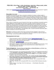
Figure 2: Contour plot of <strong>the</strong> potential VTriang. with minima shown in white.<br />
The result is a b<strong>and</strong> structure, of which Fig. 1 is an example, with <strong>the</strong> two lowest <strong>b<strong>and</strong>s</strong><br />
shown. B<strong>and</strong>s are usually separated by b<strong>and</strong>gaps, <strong>the</strong> energy of closest approach. In<br />
our example <strong>the</strong> b<strong>and</strong>gaps for <strong>the</strong> higher <strong>b<strong>and</strong>s</strong> arise from higher orders of perturbation<br />
<strong><strong>the</strong>ory</strong>.<br />
• There are energy eigenfunctions in <strong>the</strong> b<strong>and</strong> gaps – we just have to take ∆k in Eq. (3)<br />
to be imaginary i.e. exponentially growing or decaying solutions. This perspective is<br />
more often encountered when dealing with time-dependent problems of <strong>the</strong> form<br />
¨x + ω 2 0 (1 + ɛ cos Ωt) = 0,<br />
(Mathieu <strong>equation</strong>) which describes an oscillator in an oscillating quadratic potential.<br />
Translating <strong>the</strong> above results into this language shows that such an oscillator becomes<br />
unstable when its resonant frequency ω0 is close to Ω/2 (which makes sense if you<br />
think about it).<br />
2 Triangular lattice<br />
This treatment can be generalized to higher dimensions, <strong>and</strong> we turn now to <strong>the</strong> particularly<br />
interesting example of <strong>the</strong> triangular lattice. Such a lattice can be formed by <strong>the</strong> minima of<br />
<strong>the</strong> potential<br />
3<br />
VTriang.(r) = −V0 cos ki · r (5)<br />
with r = (z, x) (for reasons that will become clear shortly) <strong>and</strong> with <strong>the</strong> three vectors<br />
3<br />
i=1
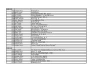
Figure 3: The shaded triangle shows <strong>the</strong> Brillouin zone in k-space. The three red K points<br />
are coupled toge<strong>the</strong>r by <strong>the</strong> perturbation, as are <strong>the</strong> three blue points (which correspond K<br />
points in <strong>the</strong> neighboring Brillouin zones)<br />
(chosen so that <strong>the</strong> resulting lattice has constant a)<br />
k1 = 4π<br />
√ 3a (0, 1)<br />
k2 = 4π<br />
√ <br />
√ 3/2, 1/2<br />
3a<br />
k3 = 4π<br />
<br />
√ −<br />
3a<br />
√ <br />
3/2, 1/2<br />
VTriang. is shown in Fig. 2. Let’s treat VTriang. using degenerate perturbation <strong><strong>the</strong>ory</strong>. After<br />
some thought we can identify three degenerate states that are coupled by <strong>the</strong> perturbation,<br />
with momenta<br />
K1 = 2π<br />
√ 3a (1, 0)<br />
K2 = 2π<br />
<br />
√ −1/2,<br />
3a<br />
√ <br />
3/2<br />
K3 = 2π<br />
<br />
√ −1/2, −<br />
3a<br />
√ <br />
3/2 , (7)<br />
<strong>and</strong> similarly for <strong>the</strong> three states related to <strong>the</strong>se by rotation through 60◦ , see Fig. 3. In <strong>the</strong><br />
basis of <strong>the</strong> plane waves eiKi·r <strong>the</strong> matrix elements of VTriang.(r) are<br />
⎛<br />
0<br />
⎝ −V0/2<br />
−V0/2<br />
0<br />
⎞<br />
−V0/2<br />
−V0/2 ⎠ , (8)<br />
−V0/2 −V0/2 0<br />
4<br />
(6)
which has eigenvalues −V0, V0/2, V0/2: <strong>the</strong> degeneracy is not lifted by <strong>the</strong> lattice potential!<br />
In o<strong>the</strong>r words, two of <strong>the</strong> <strong>b<strong>and</strong>s</strong> touch at <strong>the</strong> K-points.<br />
Now we consider moving away from <strong>the</strong> K-points, just as we moved away from ±π/a<br />
in <strong>the</strong> 1D case. If we consider <strong>the</strong> three states Ki + ∆k coupled by <strong>the</strong> lattice potential,<br />
<strong>the</strong> kinetic energies of <strong>the</strong> three are no longer equal, <strong>and</strong> this tends to lift <strong>the</strong> remaining<br />
degeneracy. This turns out to be a linear effect, so we consider <strong>the</strong> expansion<br />
⎛<br />
⎜<br />
⎝<br />
E (0)<br />
K1+∆k − E(0)<br />
K1<br />
0 E (0)<br />
K2+∆k<br />
0 0<br />
− E(0)<br />
K2<br />
0 0 E (0)<br />
K3+∆k<br />
0<br />
− E(0)<br />
K3<br />
⎞<br />
⎟<br />
⎠ ∼ 2<br />
m<br />
⎛<br />
⎝<br />
K1 · ∆k 0 0<br />
0 K2 · ∆k 0<br />
0 0 K3 · ∆k<br />
as a perturbation acting in <strong>the</strong> two dimensional degenerate subspace. The eigenvalue −V0<br />
of Eq. (8) has eigenvector (1, 1, 1)/ √ 3, while <strong>the</strong> degenerate subspace is spanned by <strong>the</strong><br />
vectors with entries adding to zero. We pick <strong>the</strong> following basis<br />
<br />
2<br />
κ+ =<br />
3 (1, −1/2, −1/2) κ− = (0, −1/ √ 2, 1/ √ 2) (10)<br />
[remember <strong>the</strong>se are not vectors in k-space, but in <strong>the</strong> subspace spanned by <strong>the</strong> plane<br />
waves e iKi·r !] If <strong>the</strong> kinetic energy matrix Eq. (9) is written 2 /m (Σz∆kz + Σx∆kx) with<br />
Σi = diag ((K1)i, (K2)i, (K3)i) , i = z, x<br />
<strong>the</strong>n one can show that <strong>the</strong> action of Σi in <strong>the</strong> subspace spanned by κ± is just (proportional<br />
to) that of <strong>the</strong> corresponding Pauli matrices<br />
Σzκ± = ± π<br />
√ 3a κ±<br />
Σxκ± = π<br />
√ 3a κ∓<br />
[be careful here – <strong>the</strong> matrices Σi of course commute in <strong>the</strong> three dimensional space: it is<br />
only <strong>the</strong>ir projection into <strong>the</strong> degenerate subspace spanned by κ± that is non-trivial]<br />
The overall conclusion is that in <strong>the</strong> <strong>b<strong>and</strong>s</strong> that touch at <strong>the</strong> K-points <strong>the</strong> kinetic energy<br />
operator Eq. (9) has <strong>the</strong> form<br />
2<br />
2<br />
(9)<br />
(11)<br />
π<br />
√ 3a (σz∆kz + σx∆kx) (12)<br />
so that just away from <strong>the</strong>se points <strong>the</strong> <strong>b<strong>and</strong>s</strong> have <strong>the</strong> structure E±(∆k) = ± 2<br />
2<br />
π<br />
√ 3a |∆k|.<br />
Eq. (12) has <strong>the</strong> form of a general symmetric 2 × 2 matrix. In fact it is just <strong>the</strong> momentum<br />
space version of a <strong>Dirac</strong> <strong>equation</strong>. Let’s write <strong>the</strong> real space wavefunction for k near one of<br />
<strong>the</strong> K points as<br />
<br />
3<br />
ψk(r) = ψ+(r) (κ+)ie iκi·r<br />
<br />
3<br />
+ ψ−(r) (κ−)ie iKi·r<br />
<br />
i=1<br />
= ψ+(r)ϕ+(r) + ψ−(r)ϕ−(r), (13)<br />
5<br />
i=1<br />
⎞<br />
⎠
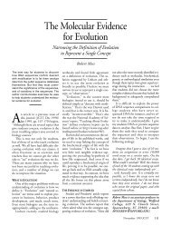
Figure 4: A, B, <strong>and</strong> C sublattices of <strong>the</strong> triangular lattice. Each sublattice forms a triangular<br />
lattice by itself, with orientation rotated by 90 ◦ <strong>and</strong> lattice constant √ 3a. Removing <strong>the</strong> points<br />
on <strong>the</strong> A sublattice leaves a honeycomb lattice formed by <strong>the</strong> B <strong>and</strong> C sites.<br />
where we identify ϕ±(r) with<br />
<br />
<strong>the</strong><br />
<br />
periodic Bloch functions for <strong>the</strong> two touching <strong>b<strong>and</strong>s</strong> (c.f.<br />
ψ+<br />
Eq. (4)). The doublet Ψ = <strong>the</strong>n satisfies two-dimensional (masless) <strong>Dirac</strong> <strong>equation</strong><br />
ψ−<br />
−i (σz∂z + σx∂x) Ψ = Eψ<br />
• Note that <strong>the</strong>re are three sublattices in <strong>the</strong> triangular lattice (see Fig. 4): removing <strong>the</strong><br />
A sites leaves behind a honeycomb lattice.<br />
Although <strong>the</strong>se lattices are two-dimensional, <strong>the</strong>y have real physical incarnations. A<br />
particularly popular material in current research is graphene, which consists of a single<br />
layer of <strong>the</strong> graphite structure of Carbon, see Fig. 5. Recent experiments on <strong>the</strong> electronic<br />
properties of <strong>the</strong>se two-dimensional structures have revealed striking evidence<br />
for <strong>the</strong> <strong>Dirac</strong> spectrum. A more detailed calculation of <strong>the</strong> b<strong>and</strong> structure is shown in<br />
Fig. 6: <strong>the</strong> <strong>Dirac</strong> cones are clearly visible. While <strong>the</strong> structure away from <strong>the</strong> cones is<br />
complicated, <strong>the</strong> position of <strong>the</strong> K-points is fixed by <strong>the</strong> lattice symmetry.<br />
• What would happen if we destroyed or reduced <strong>the</strong> symmetry of <strong>the</strong> problem, for instance<br />
by stretching <strong>the</strong> lattice slightly in one direction? Is <strong>the</strong>re still a point of degeneracy<br />
where <strong>the</strong> two <strong>b<strong>and</strong>s</strong> touch? At least for small deformations this must be true: <strong>the</strong><br />
effect of this deformation will be to introduce some additional 2 × 2 symmetric matrix<br />
into <strong>the</strong> b<strong>and</strong> Hamiltonian. Obviously this may be compensated by a shift in ∆k, so<br />
that <strong>the</strong> K-point moves. This is an example of <strong>the</strong> Wigner-von Neumann <strong>the</strong>orem: for<br />
a real symmetric Hamiltonian a degeneracy may generically be found by tuning two<br />
parameters (in this case <strong>the</strong> two components of <strong>the</strong> momentum). Contrast this situation<br />
with <strong>the</strong> 1D case, where a b<strong>and</strong>gap is <strong>the</strong> generic situation because we only have<br />
one parameter to vary. Note that for general hermitian Hamiltonians (that would result<br />
from breaking time-reversal symmetry) we would need to vary three parameters (c.f.<br />
problem 6, problem set 3).<br />
6
Figure 5: Honeycomb graphene layers of carbon atoms stacked to form graphite<br />
Figure 6: B<strong>and</strong> structure of graphene showing <strong>the</strong> <strong>Dirac</strong> (K) points arranged in a hexagon.<br />
7
• Some of <strong>the</strong> unusual properties arising from <strong>the</strong> <strong>Dirac</strong> cones are connected with <strong>the</strong><br />
phase acquired by a particle whose momentum encircles one of <strong>the</strong> K-points. This can<br />
occur due to motion in a perpendicular magnetic field, for example. Using <strong>the</strong> result of<br />
problem 6, problem set 3, we see that this phase is just ±π, <strong>and</strong> this enters into <strong>the</strong><br />
semiclassical quantization rule for <strong>the</strong> particle’s energy.<br />
8