2D Spectral Element Scheme for Viscous Burgers' Equation
2D Spectral Element Scheme for Viscous Burgers' Equation
2D Spectral Element Scheme for Viscous Burgers' Equation
You also want an ePaper? Increase the reach of your titles
YUMPU automatically turns print PDFs into web optimized ePapers that Google loves.
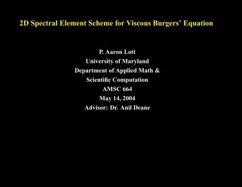
<strong>2D</strong> <strong>Spectral</strong> <strong>Element</strong> <strong>Scheme</strong> <strong>for</strong> <strong>Viscous</strong> Burgers’ <strong>Equation</strong><br />
P. Aaron Lott<br />
University of Maryland<br />
Department of Applied Math &<br />
Scientific Computation<br />
AMSC 664<br />
May 14, 2004<br />
Advisor: Dr. Anil Deane
AMSC 664: <strong>2D</strong> <strong>Spectral</strong> <strong>Element</strong> <strong>Scheme</strong> <strong>for</strong> <strong>Viscous</strong> Burgers’ <strong>Equation</strong> 2<br />
Motivation/Scientific Context<br />
● To model the dynamics of the Earth’s Mantle we treat it as a highly<br />
viscous, incompressible Boussinesq fluid.<br />
● It is important to study the affects of flows over long time periods<br />
to better constrain the parameter space of the model.<br />
● There is seismic and geochemical evidence of chemical/structural<br />
phase transition at the depth of 410 and 670 km. There are viscosity<br />
changes of several orders of magnitude. To handle these sharp<br />
interfaces one needs a refinement method to efficiently study the<br />
flow in this region.<br />
P. Aaron Lott palott@ipst.umd.edu
AMSC 664: <strong>2D</strong> <strong>Spectral</strong> <strong>Element</strong> <strong>Scheme</strong> <strong>for</strong> <strong>Viscous</strong> Burgers’ <strong>Equation</strong> 3<br />
● The Governing <strong>Equation</strong>s are:<br />
∇ · u = 0 Incompressibility<br />
Mantle Convection<br />
1<br />
ρ∇p = ν∇2u − gαΔT (Momentum <strong>Equation</strong> with∂u ∂t<br />
= 0)<br />
∂T<br />
∂t + u · ∇T = κ∇2T + J ( Thermal energy equation)<br />
ρCp<br />
● u - velocity, T - temp, p is pressure, ν -viscosity, κ - thermal<br />
diffusivity, α - thermal expansion coefficient, ρ - density, and Cp -<br />
heat capacity at constant pressure, J - rate of internal pressure per<br />
unit volume, g - gravity.<br />
● Note, these are the Incompressible Steady Stokes <strong>Equation</strong>s with<br />
a source term fed by the unsteady advection diffusion equation at<br />
each time step.<br />
P. Aaron Lott palott@ipst.umd.edu
AMSC 664: <strong>2D</strong> <strong>Spectral</strong> <strong>Element</strong> <strong>Scheme</strong> <strong>for</strong> <strong>Viscous</strong> Burgers’ <strong>Equation</strong> 4<br />
Advection Diffusion <strong>Equation</strong><br />
● We are solving the Advection Diffusion equations in 1D and <strong>2D</strong>,<br />
with advection velocityc and viscosity ν.<br />
● 1D<br />
● <strong>2D</strong><br />
∂u<br />
∂t<br />
∂u<br />
∂t<br />
+ (c∂u<br />
∂x ) = ν∂2 u<br />
∂x2 (1)<br />
= νΔu −c · ∇u in Ω t ≥ 0 (2)<br />
● Notec = u yields the viscous Burgers’ <strong>Equation</strong>s.<br />
P. Aaron Lott palott@ipst.umd.edu
AMSC 664: <strong>2D</strong> <strong>Spectral</strong> <strong>Element</strong> <strong>Scheme</strong> <strong>for</strong> <strong>Viscous</strong> Burgers’ <strong>Equation</strong> 5<br />
<strong>Spectral</strong> <strong>Element</strong> Discretization<br />
● We use a <strong>Spectral</strong> <strong>Element</strong> Method Discretization to solve 1 and 2,<br />
expanding the solution as a linear combination of basis functions<br />
φi(x).<br />
u k n =<br />
n<br />
∑ u<br />
i=0<br />
k i (t)φi(x) (3)<br />
P. Aaron Lott palott@ipst.umd.edu
AMSC 664: <strong>2D</strong> <strong>Spectral</strong> <strong>Element</strong> <strong>Scheme</strong> <strong>for</strong> <strong>Viscous</strong> Burgers’ <strong>Equation</strong> 6<br />
●<br />
Spatial Discretization- Basis Functions<br />
Figure 1: A. GLL Spatial Discretization with 2 elements and 5th degree Polynomials B. GLL Polynomials of degree 1<br />
through 10<br />
P. Aaron Lott palott@ipst.umd.edu
AMSC 664: <strong>2D</strong> <strong>Spectral</strong> <strong>Element</strong> <strong>Scheme</strong> <strong>for</strong> <strong>Viscous</strong> Burgers’ <strong>Equation</strong> 7<br />
Spatial Discretization<br />
● The discretized equation can be written as a non-linear differential<br />
equation<br />
M ˙u(t) = −C(u)u(t) − νKu(t) (4)<br />
● M- Mass matrix, K- Stiffness matrix and C(u) is the nonlinear<br />
discrete operator. Each of which are block diagonal matrices.<br />
● So to solve <strong>for</strong> u(x,t) we will integrate these equations in time.<br />
P. Aaron Lott palott@ipst.umd.edu
AMSC 664: <strong>2D</strong> <strong>Spectral</strong> <strong>Element</strong> <strong>Scheme</strong> <strong>for</strong> <strong>Viscous</strong> Burgers’ <strong>Equation</strong> 8<br />
●<br />
Spatial Discretization<br />
Figure 2: Global System Matrices. From the left 1 Mass,1, Convection, 1 Stiffness(Diffusion)<br />
P. Aaron Lott palott@ipst.umd.edu
AMSC 664: <strong>2D</strong> <strong>Spectral</strong> <strong>Element</strong> <strong>Scheme</strong> <strong>for</strong> <strong>Viscous</strong> Burgers’ <strong>Equation</strong> 9<br />
Time Discretization<br />
● In order to obtain a stable solution in time, one considers the<br />
eigenvalues of the operators acting on u, and makes certain that<br />
the time marching scheme is stable in this region.<br />
● In our system, C and K act on u<br />
●<br />
Figure 3: Eigenvalues of the Diffusion and Convection operators<br />
P. Aaron Lott palott@ipst.umd.edu
AMSC 664: <strong>2D</strong> <strong>Spectral</strong> <strong>Element</strong> <strong>Scheme</strong> <strong>for</strong> <strong>Viscous</strong> Burgers’ <strong>Equation</strong> 10<br />
Time Discretization<br />
● For spectral methods the eigenvalues, λ, of the diffusion matrix<br />
are real and negative, and the maximum eigenvalue is O(N 4 ) where<br />
N is the maximum polynomial degree. For <strong>Spectral</strong> <strong>Element</strong>s,<br />
empirical tests show λ ≈ O(neN 3 ) where ne is the number of elements.<br />
● The eigenvalues, λ, of the convection operator have an imaginary<br />
part and and a negative real part, and the largest eigenvalue is<br />
O(N 2 ).<br />
Thus, we want a time discretization which is stable on the negative<br />
real axis and the imaginary axis.<br />
P. Aaron Lott palott@ipst.umd.edu
AMSC 664: <strong>2D</strong> <strong>Spectral</strong> <strong>Element</strong> <strong>Scheme</strong> <strong>for</strong> <strong>Viscous</strong> Burgers’ <strong>Equation</strong> 11<br />
●<br />
Time Discretization<br />
Figure 4: Stability region arrows denote stability outside the corresponding curve <strong>for</strong> the Backward Difference time<br />
marching scheme.<br />
P. Aaron Lott palott@ipst.umd.edu
AMSC 664: <strong>2D</strong> <strong>Spectral</strong> <strong>Element</strong> <strong>Scheme</strong> <strong>for</strong> <strong>Viscous</strong> Burgers’ <strong>Equation</strong> 12<br />
Time Discretization<br />
● In order to achieve 3rd order accuracy, and a stable solution in<br />
time we use the BDF3 scheme, and extrapolate the Convection<br />
term at each iteration.<br />
( 11<br />
M<br />
M + νK)vn+1 i =<br />
6Δt Δt (3vni − 3<br />
2 vn−1<br />
1<br />
i +<br />
3 vn−2 i ) −Cv n+1<br />
i<br />
where we use 3rd order extrapolation to obtain<br />
Cv n+1<br />
i<br />
= 3Cvn i − 3Cv n−1<br />
i<br />
(5)<br />
+Cvn−2<br />
i + O(Δt3 ) (6)<br />
● For SEM a harsh condition is placed on Δt in order to satisfy the<br />
CFL criteria. For basis functions of degree N − 1,<br />
Δt ≤ 6.5 π<br />
ν<br />
2<br />
N4 (7)<br />
P. Aaron Lott palott@ipst.umd.edu
AMSC 664: <strong>2D</strong> <strong>Spectral</strong> <strong>Element</strong> <strong>Scheme</strong> <strong>for</strong> <strong>Viscous</strong> Burgers’ <strong>Equation</strong> 13<br />
Computation Localization<br />
● We originally <strong>for</strong>med the global system matrices, and then iterated<br />
over time. However, as we moved into <strong>2D</strong> these system matrices<br />
have size (P + 1) 2 NxNy, which, even <strong>for</strong> coarse meshes are quite<br />
large.<br />
● Static Condensation<br />
Earlier we gave an illustration of the coupling between elements.<br />
By re-ordering the mapping between local and global indices we<br />
could effectively decouple the interiors and only solve the coupled<br />
system on elemental boundaries. This could all be done with local<br />
element matrices of size (P + 1) 2 .<br />
P. Aaron Lott palott@ipst.umd.edu
AMSC 664: <strong>2D</strong> <strong>Spectral</strong> <strong>Element</strong> <strong>Scheme</strong> <strong>for</strong> <strong>Viscous</strong> Burgers’ <strong>Equation</strong> 14<br />
●<br />
Computation Localization<br />
Figure 5: Coupled and Uncoupled Diffusion operator. 1 Big coupled 1 Boundary 1Interior<br />
P. Aaron Lott palott@ipst.umd.edu
AMSC 664: <strong>2D</strong> <strong>Spectral</strong> <strong>Element</strong> <strong>Scheme</strong> <strong>for</strong> <strong>Viscous</strong> Burgers’ <strong>Equation</strong> 15<br />
Computation Localization<br />
● Advantages:<br />
Reduces communication once the boundary in<strong>for</strong>mation has been<br />
decoupled. No global matrices need to be stored, all calculations<br />
are done on element matrices<br />
● Disadvantages: Need to compute Schur compliment.<br />
P. Aaron Lott palott@ipst.umd.edu
AMSC 664: <strong>2D</strong> <strong>Spectral</strong> <strong>Element</strong> <strong>Scheme</strong> <strong>for</strong> <strong>Viscous</strong> Burgers’ <strong>Equation</strong> 16<br />
Computation Localization<br />
● <strong>Element</strong>wise operations<br />
Instead of using static condensation, one can per<strong>for</strong>m operations<br />
on local elements and then cleverly add the proper amount to the<br />
global solution U without the cost of static condensation.<br />
● A weighting matrix is <strong>for</strong>med <strong>for</strong> each element to determine the<br />
contribution of the local solution to the global solution. Finally we<br />
take care of the element boundary dependencies after each local<br />
calculation.<br />
P. Aaron Lott palott@ipst.umd.edu
AMSC 664: <strong>2D</strong> <strong>Spectral</strong> <strong>Element</strong> <strong>Scheme</strong> <strong>for</strong> <strong>Viscous</strong> Burgers’ <strong>Equation</strong> 17<br />
Computation Localization<br />
● Advantages: For large P this should be very efficient since most<br />
entries are interior nodes, and each processor can use its cache<br />
more efficiently. No global matrices need to be stored, all calculations<br />
are done on element matrices<br />
● Disadvantages: For small polynomial degree, more communication<br />
compared to calculations<br />
P. Aaron Lott palott@ipst.umd.edu
AMSC 664: <strong>2D</strong> <strong>Spectral</strong> <strong>Element</strong> <strong>Scheme</strong> <strong>for</strong> <strong>Viscous</strong> Burgers’ <strong>Equation</strong> 18<br />
Computation Localization<br />
● In either case, these problems scale well to higher dimensions because<br />
the global Matrix operators can be written as tensor products.<br />
● We construct the local operators <strong>for</strong> all possible polynomial degree<br />
(run time parameter), and store them in an easily accessible<br />
efficient data structure. These include, M,A,C, Derivative, Iterpolants<br />
from Pn → Pn−1 and vice versa. These structures are accessible<br />
through a global data module.<br />
P. Aaron Lott palott@ipst.umd.edu
AMSC 664: <strong>2D</strong> <strong>Spectral</strong> <strong>Element</strong> <strong>Scheme</strong> <strong>for</strong> <strong>Viscous</strong> Burgers’ <strong>Equation</strong> 19<br />
P-type Refinement<br />
● With the local matrices stored <strong>for</strong> all values of P, and the ability<br />
to per<strong>for</strong>m local operations and build the global solution, it is now<br />
trivial to compute the derivative of the local solution and per<strong>for</strong>m<br />
error analysis with it.<br />
● For example, if the slope of our solution at a local element is<br />
greater than some user defined value, then we increase the polynomial<br />
degree of that element by one.<br />
● We per<strong>for</strong>m this on each element and then construct a new local<br />
to global mapping with respect to the new elements.<br />
P. Aaron Lott palott@ipst.umd.edu
AMSC 664: <strong>2D</strong> <strong>Spectral</strong> <strong>Element</strong> <strong>Scheme</strong> <strong>for</strong> <strong>Viscous</strong> Burgers’ <strong>Equation</strong> 20<br />
●<br />
P-type Refinement<br />
Figure 6: 3 time steps in solution to burgers’ equation starting with N=32 P=4 refining with abs(du/dx) is greater<br />
than 8<br />
P. Aaron Lott palott@ipst.umd.edu
AMSC 664: <strong>2D</strong> <strong>Spectral</strong> <strong>Element</strong> <strong>Scheme</strong> <strong>for</strong> <strong>Viscous</strong> Burgers’ <strong>Equation</strong> 21<br />
● 1D Burgers’s <strong>Equation</strong><br />
Validation<br />
Figure 7: Comparison of Results between Our code (left) and Published Code (right)<br />
P. Aaron Lott palott@ipst.umd.edu
AMSC 664: <strong>2D</strong> <strong>Spectral</strong> <strong>Element</strong> <strong>Scheme</strong> <strong>for</strong> <strong>Viscous</strong> Burgers’ <strong>Equation</strong> 22<br />
●<br />
Validation<br />
Figure 8: Comparison of results between our code and actual maximum amplitude of slope. We have a value of<br />
152.2265 at t=.5100 analytical value is 152.0051 at t=.5105. The compares very well with other published numerical<br />
methods.<br />
P. Aaron Lott palott@ipst.umd.edu
AMSC 664: <strong>2D</strong> <strong>Spectral</strong> <strong>Element</strong> <strong>Scheme</strong> <strong>for</strong> <strong>Viscous</strong> Burgers’ <strong>Equation</strong> 23<br />
● <strong>2D</strong> Burgers’s <strong>Equation</strong><br />
Start with initial conditions<br />
<strong>2D</strong> Results<br />
u(x,y,0) = .01 4(x2 +y 2 )<br />
on[−1,1] 2<br />
We use periodic boundary conditions, P = 8, Nx = 4, Ny = 4 ν =<br />
.01<br />
P. Aaron Lott palott@ipst.umd.edu<br />
(8)
AMSC 664: <strong>2D</strong> <strong>Spectral</strong> <strong>Element</strong> <strong>Scheme</strong> <strong>for</strong> <strong>Viscous</strong> Burgers’ <strong>Equation</strong> 24<br />
● Add <strong>2D</strong> adaptivity<br />
● Implement Stokes <strong>Equation</strong><br />
● Parallelization<br />
Future Directions<br />
● Preconditioned Conjugate Gradient to solve local systems<br />
P. Aaron Lott palott@ipst.umd.edu
AMSC 664: <strong>2D</strong> <strong>Spectral</strong> <strong>Element</strong> <strong>Scheme</strong> <strong>for</strong> <strong>Viscous</strong> Burgers’ <strong>Equation</strong> 25<br />
Conclusions/Summary<br />
● Implemented and verified 1D and <strong>2D</strong> viscous Burgers’ <strong>Equation</strong><br />
● Implemented P adaptivity in 1D, and framework <strong>for</strong> adaptivity in<br />
<strong>2D</strong><br />
● Structured code to begin MPI Parallelization<br />
P. Aaron Lott palott@ipst.umd.edu
AMSC 664: <strong>2D</strong> <strong>Spectral</strong> <strong>Element</strong> <strong>Scheme</strong> <strong>for</strong> <strong>Viscous</strong> Burgers’ <strong>Equation</strong> 26<br />
References<br />
● [1] High-Order Methods <strong>for</strong> Incompressible Fluid Flows. M.O.<br />
Deville, P.F. Fischer, E.H. Mund. Cambridge University Press<br />
2002.<br />
[2] An overlapping Schwarz method <strong>for</strong> spectral element solution<br />
of the incompressible Navier-Stokes equations. P.F. Fischer. Journal<br />
of Computational Physics 1997.<br />
[3] <strong>Spectral</strong>/hp <strong>Element</strong> Methods <strong>for</strong> CFD. G.E. Karniadakis, S.J.<br />
Sherwin. Ox<strong>for</strong>d University Press 1999.<br />
[4] An Adaptive Finite <strong>Element</strong> <strong>Scheme</strong> <strong>for</strong> Transient Problems<br />
in CFD. Rainald Löhner. Computational Methods in Applied Mechanics<br />
and Engineering. 61 (1987) 323-338<br />
[5] <strong>Spectral</strong> element methods: theory and applications. F.N. van<br />
de Vosee, P.D. Minev.<br />
http://www.mate.tue.nl/people/vosse/docs/vosse96b.pdf
AMSC 664: <strong>2D</strong> <strong>Spectral</strong> <strong>Element</strong> <strong>Scheme</strong> <strong>for</strong> <strong>Viscous</strong> Burgers’ <strong>Equation</strong> 27<br />
[6] Project Website. http://www.lcv.umd.edu/ palott/research/graduate/66<br />
P. Aaron Lott palott@ipst.umd.edu
AMSC 664: <strong>2D</strong> <strong>Spectral</strong> <strong>Element</strong> <strong>Scheme</strong> <strong>for</strong> <strong>Viscous</strong> Burgers’ <strong>Equation</strong> 28<br />
● 2<br />
Figures<br />
P. Aaron Lott palott@ipst.umd.edu
AMSC 664: <strong>2D</strong> <strong>Spectral</strong> <strong>Element</strong> <strong>Scheme</strong> <strong>for</strong> <strong>Viscous</strong> Burgers’ <strong>Equation</strong> 29<br />
● 2<br />
Figures<br />
P. Aaron Lott palott@ipst.umd.edu
AMSC 664: <strong>2D</strong> <strong>Spectral</strong> <strong>Element</strong> <strong>Scheme</strong> <strong>for</strong> <strong>Viscous</strong> Burgers’ <strong>Equation</strong> 30<br />
● 2<br />
Figures<br />
P. Aaron Lott palott@ipst.umd.edu
AMSC 664: <strong>2D</strong> <strong>Spectral</strong> <strong>Element</strong> <strong>Scheme</strong> <strong>for</strong> <strong>Viscous</strong> Burgers’ <strong>Equation</strong> 31<br />
● 5<br />
Figures<br />
P. Aaron Lott palott@ipst.umd.edu
AMSC 664: <strong>2D</strong> <strong>Spectral</strong> <strong>Element</strong> <strong>Scheme</strong> <strong>for</strong> <strong>Viscous</strong> Burgers’ <strong>Equation</strong> 32<br />
● 5<br />
Figures<br />
P. Aaron Lott palott@ipst.umd.edu
AMSC 664: <strong>2D</strong> <strong>Spectral</strong> <strong>Element</strong> <strong>Scheme</strong> <strong>for</strong> <strong>Viscous</strong> Burgers’ <strong>Equation</strong> 33<br />
● 5<br />
Figures<br />
The End — Thank you


