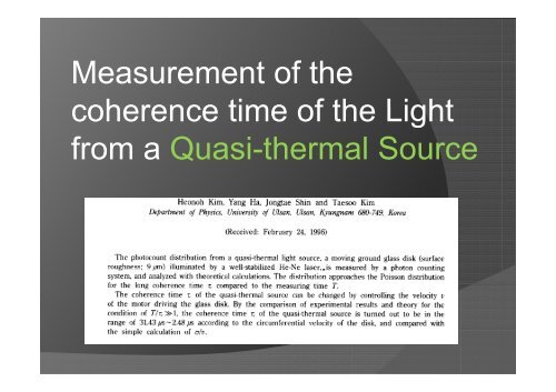
Measurement of the coherence time of the Light from a Quasi ...

MMeasurement t of f the th
coherence time of the Light
from a Quasi-thermal Source

Chaotic light
(thermal cavity, filament lamp)
The different atoms are excited by an
electrical discharge and emit their radiation
independently of one another.
The shape of an emission line is determined
by the statistical spread in atomic velocities
and the random occurrence of collisions.
Δ Δνν
1
Generally,
Δ Δνν = − 12 ττ c
τ
τ c ≤
10 s
c

collision τ2 collision τ1 collision
Lorentzian
lineshape
collision-broadened lli i b d d li light h source
Gaussian
lineshape
Doppler broadening light source

Used rotating ground glass disk
(surface roughness: 9㎛)
QQuasi-thermal i th l SSource
It has property of chaos light, but
coherence time is longer than
chaos light. g
τc of the quasi-thermal source
can be changed by controlling
the velocity y v of the motor driving g
the glass disk.
τ =
c
σ σ (surface ( roughness) g )
v
(rotating speed)

I (, tT) is the mean intensity that falls on the phototube during
the period from t to t+T, then,
1 t+ T
I ( t t, T ) = ∫ I ( t ) dt dt′
T ∫t
The probability of detecting n number of photons during time duration
T is
P ( T ) = P ( t, T )
n n
n
⎡⎣⎡ζζI (, t T ) T⎤⎦⎤
=
⎣ ⎦
exp ⎡ ⎡ζI( t, T) T ⎤
n!
⎣ ⎦
This result is Known as the Mandel formula. ζ
(efficiency of detector)

So Mean number of photocounts is
∞
∑
= 0
n = nPP ( T ) = ζζ I ( t, TT T) ) T = ζζIT
IT
n
n
And the second moment of the distribution given by
∞
2 2
n ∑ ∑nPT
n ( ) ζζI ( tTT , ) ζζI(
( tTT , )
n=
0
= = + ⎡ ⎣ ⎤ ⎦
= n + ⎣⎡ζI(, t T) T⎦⎤
2
The variance of the photocount distribution is therefore
2 2 2
2 2 ( ) ( 2 2
Δ n = n − n = n + ζ T I(, t T) −I
)
2

Line width γ(1/ τ )
= Lorentzian lineshape function
Its second order coherence function is, is
(2) −2γ
τ
g ( τ ) = 1+
e
The average of integration time T is
c
T T
1
∫∫
−2γγ t −t
− = ∫∫ 2
1 2
T
2
(2) ( )
2 1
g (0) 1 e dtdt
0 0
1 −2γT
= ⎡e + 2γT −1⎤
2 2
2γ
T ⎣ ⎦
g
(2)
(0)
=
I(, t T)
I
2

( )
2
2 n −2γT
Δ n = n + ⎡e + 2γT −1⎤
2 2
2 2γγ T ⎣ ⎦
T > τ c
T ττ
c
( )
2
Δ n = n + n
( ) 2 n
n n
2
2
T τ c
Δ = + ( )
γT
2
Δ n =
n

Measurement time : T Redline: pulse
T T T T T T T T T T
0 1 2 3 4 5 6 7 8 9 10
Photocount
10,000 times
t

Measurement time : T (fixed: 10 μs) =4
Voltage change (velocity of the motor driving) :
τc change

Variance of ( ) by the velocity v
2
Variance of ( Δ n n)
by the velocity v
v (rotating speed) (m/s)

T=50 T 50 μs
T=30 μs
T=20 μs
τ
c
σ( = 9 μm)
v
= ( )
2 τ c n
Δ n = n +
T
2