SISIS Josephson transistor in the nonequilibrium regime - Low ...
SISIS Josephson transistor in the nonequilibrium regime - Low ...
SISIS Josephson transistor in the nonequilibrium regime - Low ...

Create successful ePaper yourself
Turn your PDF publications into a flip-book with our unique Google optimized e-Paper software.
Hels<strong>in</strong>ki University of Technology Special assignment<br />
Department of Eng<strong>in</strong>eer<strong>in</strong>g Physics Tfy-3.393 Computational Physics<br />
and Ma<strong>the</strong>matics 30th August 2006<br />
<strong>SISIS</strong> <strong>Josephson</strong> <strong>transistor</strong> <strong>in</strong> <strong>the</strong> <strong>nonequilibrium</strong> <strong>regime</strong><br />
Matti Laakso<br />
62975L
Contents<br />
1 Introduction 3<br />
2 Formalism 4<br />
2.1 General concepts . . . . . . . . . . . . . . . . . . . . . . . . . . . 4<br />
2.1.1 Superconductivity . . . . . . . . . . . . . . . . . . . . . . 4<br />
2.1.2 Energy <strong>nonequilibrium</strong> . . . . . . . . . . . . . . . . . . . . 5<br />
2.2 <strong>SISIS</strong> <strong>transistor</strong> . . . . . . . . . . . . . . . . . . . . . . . . . . . . 5<br />
2.3 Quasiclassical Green’s functions . . . . . . . . . . . . . . . . . . . 6<br />
3 Equations 8<br />
3.1 K<strong>in</strong>etic equations . . . . . . . . . . . . . . . . . . . . . . . . . . . 8<br />
3.2 Green functions . . . . . . . . . . . . . . . . . . . . . . . . . . . . 10<br />
3.3 Order parameter and observables . . . . . . . . . . . . . . . . . . 12<br />
4 Results 13<br />
4.1 Full nonequlibrium . . . . . . . . . . . . . . . . . . . . . . . . . . 13<br />
4.2 Relaxation-time approximation . . . . . . . . . . . . . . . . . . . 19<br />
4.3 Collision <strong>in</strong>tegral . . . . . . . . . . . . . . . . . . . . . . . . . . . 20<br />
4.4 Asymmetric structure . . . . . . . . . . . . . . . . . . . . . . . . 22<br />
4.4.1 Sp<strong>in</strong>-flip scatter<strong>in</strong>g . . . . . . . . . . . . . . . . . . . . . . 26<br />
5 Discussion 27<br />
A Tunnel<strong>in</strong>g rate 29<br />
B Ambegaokar-Baratoff formula for <strong>the</strong> critical current 30<br />
2
1 Introduction<br />
Mesoscopic physics deals with phenomena <strong>in</strong> systems which are small enough<br />
<strong>in</strong> size to exhibit quantum mechanical properties, but sufficiently large that <strong>the</strong><br />
need to take <strong>in</strong>dividual atoms <strong>in</strong>to account does not arise. In general this means<br />
structures with spatial dimensions of nanometer and micrometer scale. Mesoscopic<br />
experiments usually aim to study electron transport <strong>in</strong> small metallic<br />
wires and metal-to-metal contacts, quantum mechanics of relaxation and lowtemperature<br />
phenomena. The central concept is often <strong>the</strong> energy distribution<br />
of mesoscopic electron systems, which <strong>in</strong> <strong>the</strong>rmal equilibrium def<strong>in</strong>es <strong>the</strong> temperature<br />
of <strong>the</strong> electron gas <strong>in</strong> <strong>the</strong> sample. Also <strong>nonequilibrium</strong> distributions<br />
are often encountered and utilized <strong>in</strong> mesoscopic systems. The ability to control<br />
and measure electron distributions can be used <strong>in</strong> various device concepts, such<br />
as electronic refrigerators, <strong>the</strong>rmometers, radiation detectors and novel types of<br />
<strong>transistor</strong>s. Typically <strong>the</strong> resolution of <strong>the</strong>se devices requires <strong>the</strong> m<strong>in</strong>imization<br />
of <strong>the</strong>rmal noise and fluctuations which can be achieved at cryogenic temperatures.<br />
A practical threshold of temperature is given by <strong>the</strong> liquefaction of<br />
helium at 4.2 K.<br />
Many metals turn superconduct<strong>in</strong>g at <strong>the</strong>se temperatures, an example of<br />
quantum mechanical phenomenon which gives rise to macroscopic effects. The<br />
most famous property of superconductors is probably its ability to carry electric<br />
current without dissipation, i.e., without <strong>in</strong>duc<strong>in</strong>g a voltage drop. This is also<br />
known as supercurrent. Ano<strong>the</strong>r property is <strong>the</strong> Meissner effect, <strong>in</strong> which an<br />
external magnetic field creates eddy currents on <strong>the</strong> surface of <strong>the</strong> superconductor.<br />
These circulat<strong>in</strong>g currents create an oppos<strong>in</strong>g magnetic field with <strong>the</strong><br />
result that <strong>the</strong> total magnetic field is unable to penetrate <strong>in</strong>to <strong>the</strong> superconductor.<br />
The most important superconduct<strong>in</strong>g effect <strong>in</strong> mesoscopic systems is <strong>the</strong><br />
<strong>Josephson</strong> effect which allows <strong>the</strong> supercurrent to flow through a weak l<strong>in</strong>k, e.g.<br />
an <strong>in</strong>sulat<strong>in</strong>g barrier, between two superconductors. These <strong>Josephson</strong> junctions<br />
are very versatile objects due to <strong>the</strong>ir nonl<strong>in</strong>ear current-voltage characteristics.<br />
A particular application of <strong>Josephson</strong> junctions is <strong>the</strong> <strong>Josephson</strong> <strong>transistor</strong>,<br />
which has been a subject of recent <strong>in</strong>terest <strong>in</strong> nanoelectronics. Its latest type is<br />
composed of superconduct<strong>in</strong>g (S) and normal (N) metals separated with <strong>in</strong>sulat<strong>in</strong>g<br />
oxide barriers (I). By arrang<strong>in</strong>g <strong>the</strong>se constituents <strong>in</strong> a SINIS structure<br />
<strong>the</strong> magnitude of <strong>the</strong> supercurrent flow<strong>in</strong>g through <strong>the</strong> system can be <strong>in</strong>creased<br />
as well as suppressed by driv<strong>in</strong>g <strong>the</strong> energy distribution <strong>in</strong> <strong>the</strong> normal metal out<br />
of equilibrium [1]. This <strong>transistor</strong>like operation with large current and power<br />
ga<strong>in</strong> has also been experimentally demonstrated [2]. Also an all superconduct<strong>in</strong>g<br />
device has been proposed, where <strong>the</strong> supercurrent is controlled by voltage<br />
bias<strong>in</strong>g <strong>the</strong> middle electrode of an <strong>SISIS</strong> l<strong>in</strong>e. This has been <strong>the</strong>oretically addressed<br />
<strong>in</strong> <strong>the</strong> quasiequilibrium <strong>regime</strong> <strong>in</strong> Ref. [3]. The <strong>SISIS</strong> <strong>transistor</strong> benefits<br />
from sharp characteristics brought by <strong>the</strong> superconduct<strong>in</strong>g <strong>in</strong>terelectrode which<br />
leads to improved operational properties.<br />
In this work we study <strong>the</strong> <strong>SISIS</strong> <strong>transistor</strong> <strong>in</strong> full <strong>nonequilibrium</strong>, as well<br />
as with different strengths of energy relaxation. We also exam<strong>in</strong>e <strong>the</strong> effects of<br />
asymmetry <strong>in</strong> <strong>the</strong> <strong>SISIS</strong> l<strong>in</strong>e driv<strong>in</strong>g <strong>the</strong> energy distribution out of equilibrium.<br />
General concepts and <strong>the</strong> formalism used is <strong>in</strong>troduced <strong>in</strong> Sec. 2. Relevant equations<br />
are derived <strong>in</strong> Sec. 3. We f<strong>in</strong>ish by present<strong>in</strong>g <strong>the</strong> results and discussion<br />
<strong>in</strong> Secs. 4 and 5.<br />
3
2 Formalism<br />
2.1 General concepts<br />
2.1.1 Superconductivity<br />
The microscopic <strong>the</strong>ory of superconductivity was established <strong>in</strong> 1957 by Bardeen,<br />
Cooper and Schrieffer (BCS). Accord<strong>in</strong>g to it even a weak attractive <strong>in</strong>teraction<br />
can b<strong>in</strong>d electrons <strong>in</strong>to a bound state called <strong>the</strong> Cooper pair. This attractive<br />
<strong>in</strong>teraction arises from <strong>the</strong> polarization of <strong>the</strong> medium by a first electron attract<strong>in</strong>g<br />
positive lattice ions, which <strong>in</strong> turn attract <strong>the</strong> second electron. S<strong>in</strong>ce <strong>the</strong>se<br />
lattice deformations are phonons, <strong>the</strong> strength of <strong>the</strong> attraction is heavily dependent<br />
on temperature and vanishes completely above a material specific critical<br />
temperature TC (typically a few Kelv<strong>in</strong> for conventional superconductors, such<br />
as Al, Nb, Pb or Sn). This collective behaviour results <strong>in</strong> a condensate of Cooper<br />
pairs, which may be described with a s<strong>in</strong>gle macroscopic wavefunction. Central<br />
to this model is <strong>the</strong> assumption that <strong>the</strong> overall <strong>in</strong>teraction between <strong>the</strong> electrons<br />
is attractive up to energy differences of <strong>the</strong> order of Debye frequency, which<br />
characterizes <strong>the</strong> cutoff of <strong>the</strong> phonon frequency spectrum <strong>in</strong> solids. Therefore<br />
only electrons with<strong>in</strong> <strong>the</strong> Debye frequency around <strong>the</strong> Fermi level will take part<br />
<strong>in</strong> form<strong>in</strong>g <strong>the</strong> condensate. This is also called <strong>the</strong> BCS cutoff energy.<br />
A certa<strong>in</strong> amount of energy, 2∆, is required to break a pair and create two<br />
“normal-state” electron excitations. This leaves two holes <strong>in</strong> <strong>the</strong> Fermi sea<br />
which can also be <strong>in</strong>terpreted as two excitations of positively charged particles.<br />
These excitations are collectively called quasiparticles. Because <strong>the</strong> m<strong>in</strong>imum<br />
excitation energy of a quasiparticle from <strong>the</strong> BCS ground state is ∆, <strong>the</strong> energy<br />
spectrum has an energy gap <strong>in</strong> which <strong>the</strong>re are no states. Electrons with energies<br />
fall<strong>in</strong>g <strong>in</strong>side <strong>the</strong> gap prefer to form a Cooper pair. The density of states <strong>in</strong> BCS<strong>the</strong>ory<br />
is<br />
|E|<br />
g(E) = g0<br />
θ(|E| − |∆|),<br />
E2 − |∆| 2<br />
where g0 is <strong>the</strong> density of states at <strong>the</strong> Fermi level when <strong>the</strong> sample is <strong>in</strong> <strong>the</strong><br />
normal state and θ is <strong>the</strong> Heaviside step function. The magnitude of <strong>the</strong> energy<br />
gap at T = 0 is found to be related to <strong>the</strong> critical temperature through ∆0 =<br />
1.764 TC. 1<br />
In 1962 <strong>Josephson</strong> predicted that an electric current carried by Cooper pairs<br />
(i.e., supercurrent) should flow between two superconductors <strong>in</strong> a weak contact,<br />
usually separated with a th<strong>in</strong> <strong>in</strong>sulat<strong>in</strong>g barrier which only allows <strong>the</strong><br />
Cooper pairs to tunnel across it. Such a junction is called an SIS junction<br />
(Superconductor-Insulator-Superconductor). The magnitude of <strong>the</strong> supercurrent<br />
is given by <strong>the</strong> dc <strong>Josephson</strong> relation<br />
I = IC s<strong>in</strong>(∆χ), (1)<br />
where ∆χ is <strong>the</strong> difference across <strong>the</strong> junction <strong>in</strong> <strong>the</strong> phase of <strong>the</strong> order parameter<br />
to be def<strong>in</strong>ed later and IC is <strong>the</strong> maximum supercurrent that <strong>the</strong> junction can<br />
support. If <strong>the</strong> current driven through <strong>the</strong> junction exceeds IC, a voltage starts<br />
to appear, and <strong>the</strong> phase difference evolves <strong>in</strong> time accord<strong>in</strong>g to ∂t∆χ = 2eV .<br />
1 Throughout this text we use units <strong>in</strong> which = kB = c = 1.<br />
4
This leads to <strong>the</strong> ac <strong>Josephson</strong> relation<br />
I = IC s<strong>in</strong>(∆χ(0) + 2eV t), (2)<br />
i.e. <strong>the</strong> current through a <strong>Josephson</strong> junction with an applied dc voltage oscillates<br />
<strong>in</strong> time. For a more thorough review of superconductivity and related<br />
effects, see for example <strong>the</strong> book by T<strong>in</strong>kham [4].<br />
2.1.2 Energy <strong>nonequilibrium</strong><br />
Macroscopic electron systems <strong>in</strong> <strong>the</strong>rmal equilibrium can be described with <strong>the</strong><br />
Fermi-Dirac distribution function<br />
f 0 1<br />
(E) =<br />
exp((E − µ)/T) + 1 ,<br />
where µ is <strong>the</strong> chemical potential and T is <strong>the</strong> temperature. Consider a sample<br />
connected to large leads act<strong>in</strong>g as reservoirs of electrons. The sample assumes an<br />
equilibrium distribution with a temperature equal to <strong>the</strong> reservoirs and a chemical<br />
potential profile that depends on <strong>the</strong> voltage applied across it. The charge<br />
carriers that enter <strong>the</strong> sample due to <strong>the</strong> potential difference scatter from <strong>the</strong><br />
impurities, lattice dislocations, phonons and o<strong>the</strong>r electrons, <strong>the</strong>reby <strong>the</strong>rmaliz<strong>in</strong>g<br />
with <strong>the</strong> underly<strong>in</strong>g lattice and ma<strong>in</strong>ta<strong>in</strong><strong>in</strong>g <strong>the</strong>rmal equilibrium. The mean<br />
free path that <strong>the</strong> electron travels before scatter<strong>in</strong>g is characterized by scatter<strong>in</strong>g<br />
lengths lel for elastic scatter<strong>in</strong>g and le−ph and le−e for <strong>in</strong>elastic electronphonon<br />
and electron-electron scatter<strong>in</strong>g, respectively. In mesoscopic systems<br />
typical orders of magnitude are lel ≈ 10 . . .100 nm and le−e ≈ 1 . . .20 µm. The<br />
electron-phonon scatter<strong>in</strong>g length depends strongly on temperature. At 1 K<br />
le−ph ≈ 21 µm but at 100 mK we already have le−ph ≈ 670 µm [5].<br />
If <strong>the</strong> spatial dimensions of <strong>the</strong> sample satisfy lel ≪ L, <strong>the</strong> distribution function<br />
is described by <strong>the</strong> semiclassical Boltzmann equation <strong>in</strong> a diffusive wire<br />
with source and s<strong>in</strong>k terms called <strong>the</strong> collision <strong>in</strong>tegrals describ<strong>in</strong>g <strong>the</strong> various<br />
scatter<strong>in</strong>g processes. In <strong>the</strong> so called quasiequilibrium limit, le−e ≪ L ≪ le−ph,<br />
<strong>the</strong> electron-phonon <strong>in</strong>teraction is nearly absent and <strong>the</strong> sample can be considered<br />
as detached from <strong>the</strong> phonon bath. The high frequency of electron-electron<br />
collisions still serves as a method of relaxation and <strong>the</strong> electrons assume a Fermi<br />
distribution but with a temperature that <strong>in</strong> general differs from <strong>the</strong> temperature<br />
of <strong>the</strong> phonon bath [5]. If <strong>the</strong> sample is small enough with L ≪ le−e, le−ph,<br />
<strong>the</strong> <strong>in</strong>jected electrons are not able to relax even through collisions with o<strong>the</strong>r<br />
electrons <strong>in</strong> <strong>the</strong> sample, and <strong>the</strong> distribution may deviate strongly from <strong>the</strong><br />
Fermi function. This is called <strong>the</strong> <strong>nonequilibrium</strong> limit and we may neglect <strong>the</strong><br />
<strong>in</strong>elastic scatter<strong>in</strong>g altoge<strong>the</strong>r. In <strong>the</strong> <strong>nonequilibrium</strong> limit <strong>the</strong> concept of temperature<br />
is rendered obsolete because it is def<strong>in</strong>ed through <strong>the</strong> Fermi equilibrium<br />
distribution. However, it is still possible to def<strong>in</strong>e some effective temperature<br />
with <strong>the</strong> shape of <strong>the</strong> distribution function or <strong>the</strong> magnitude of <strong>the</strong> energy gap,<br />
for example, but <strong>the</strong>se are by no means unambiguous. The <strong>nonequilibrium</strong> form<br />
of <strong>the</strong> distribution shows up <strong>in</strong> many observable properties of <strong>the</strong> system, e.g.,<br />
current-voltage (I-V) characteristics and current noise.<br />
2.2 <strong>SISIS</strong> <strong>transistor</strong><br />
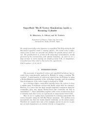
The superconduct<strong>in</strong>g structure under study is schematically depicted <strong>in</strong> Fig. 1.<br />
It consists of two cross<strong>in</strong>g <strong>SISIS</strong> l<strong>in</strong>es with a common central superconductor.<br />
5
R1<br />
µ = 0<br />
5 R5<br />
1 3<br />
2<br />
µ = 0<br />
4<br />
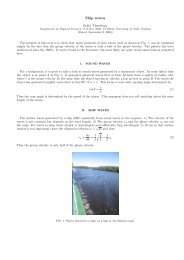
Figure 1: The <strong>SISIS</strong> structure studied <strong>in</strong> this work. The superconduct<strong>in</strong>g island<br />
<strong>in</strong> <strong>the</strong> middle (2) is connected with tunnel contacts to four large superconduct<strong>in</strong>g<br />
leads (1,3,4 and 5). The control l<strong>in</strong>e is biased with voltage V , which controls<br />
<strong>the</strong> energy distribution <strong>in</strong> <strong>the</strong> island. A supercurrent IS is driven across <strong>the</strong><br />
island from lead 4 to 5, and its magnitude depends on <strong>the</strong> distribution function<br />
<strong>in</strong> <strong>the</strong> island.<br />
The superconduct<strong>in</strong>g island <strong>in</strong> <strong>the</strong> middle is assumed to have small dimensions<br />
so that L ≪ le−e, le−ph, i.e., <strong>the</strong> energy relaxation via <strong>in</strong>elastic scatter<strong>in</strong>g is <strong>in</strong><br />
practice very weak. Each of <strong>the</strong> SIS-junctions is characterized by a junction<br />
resistance Ri, which is at least hundreds of Ohm. In contrast, <strong>the</strong> normal-state<br />
resistances of <strong>the</strong> superconductors are typically of <strong>the</strong> order 1Ω. We bias <strong>the</strong> first<br />
<strong>SISIS</strong> l<strong>in</strong>e with an adjustable voltage V , thus creat<strong>in</strong>g an energy <strong>nonequilibrium</strong><br />
<strong>in</strong> <strong>the</strong> island, and drive a supercurrent through <strong>the</strong> second <strong>SISIS</strong> l<strong>in</strong>e, which<br />
is kept at zero chemical potential. The magnitude of <strong>the</strong> supercurrent may<br />
be controlled with <strong>the</strong> external voltage, so this structure works basically as a<br />
<strong>transistor</strong>. Study<strong>in</strong>g this dependence is <strong>the</strong> ma<strong>in</strong> objective of this work.<br />
2.3 Quasiclassical Green’s functions<br />
In quantum mechanics Green’s function describes <strong>the</strong> propagation of disturbances<br />
<strong>in</strong> which a s<strong>in</strong>gle particle is added to a many-particle equilibrium system<br />
at x1 and removed at x2. Here x = (r, t) represents both space and time coord<strong>in</strong>ates.<br />
The retarded Green function describes <strong>the</strong> propagation from past to<br />
present (t1 < t2) and <strong>the</strong> advanced Green function describes <strong>the</strong> propagation<br />
from future to present time (t1 > t2). If <strong>the</strong> retarded and advanced Green<br />
function for a system is known, it is possible to calculate all energy-dependent<br />
quantities of <strong>the</strong> system, e.g., density of states. These can <strong>the</strong>n be related to<br />
<strong>the</strong> equilibrium properties of <strong>the</strong> system, such as supercurrent. In BCS-<strong>the</strong>ory<br />
6<br />
IS<br />
R4<br />
R3<br />
V
<strong>the</strong> Green function is a 2 × 2 matrix <strong>in</strong> <strong>the</strong> particle-hole (Nambu) space of <strong>the</strong><br />
form<br />
<br />
ˆG(x1,<br />
G(x1, x2)<br />
x2) =<br />
−F<br />
F(x1, x2)<br />
† (x1, x2)<br />
<br />
G(x1, ¯ .<br />
x2)<br />
(3)<br />
Here G is <strong>the</strong> Green function of <strong>the</strong> propagat<strong>in</strong>g electron, ¯ G is <strong>the</strong> Green function<br />
of <strong>the</strong> propagat<strong>in</strong>g hole and F is <strong>the</strong> pair amplitude, which is coupled to <strong>the</strong><br />
pair potential ∆ with<br />
∆(x1) = λ lim F(x2, x1). (4)<br />
x2→x1<br />
Here λ is a parameter characteriz<strong>in</strong>g <strong>the</strong> strength of <strong>the</strong> attractive <strong>in</strong>teraction.<br />
The pair potential measures <strong>the</strong> amount of correlations between <strong>the</strong> pairs of<br />
electrons and it is also called <strong>the</strong> order parameter of <strong>the</strong> superconductor. The<br />
pair amplitude and pair potential are complex functions, and <strong>the</strong> magnitude<br />
of <strong>the</strong> pair potential |∆| co<strong>in</strong>cides with <strong>the</strong> energy gap of <strong>the</strong> superconductor.<br />
In bulk superconductors |∆| is often spatially constant, but <strong>the</strong> phase χ may<br />
vary <strong>in</strong> space. This phase difference gives rise to <strong>the</strong> supercurrent. In normal<br />
metals λ = 0 and <strong>the</strong> pair potential vanishes, but it is possible for a normal<br />
metal to have a nonzero pair amplitude <strong>in</strong> a small region <strong>in</strong> good contact with<br />
a superconductor. This is called <strong>the</strong> proximity effect.<br />
Green’s functions can be found as <strong>the</strong> solutions of <strong>the</strong> Gor’kov equations.<br />
In nonstationary processes <strong>the</strong> physical system may be out of equilibrium and<br />
we need to know <strong>the</strong> exact distribution of <strong>the</strong> excitations <strong>in</strong> addition to <strong>the</strong>ir<br />
spectrum. For this we need <strong>the</strong> real-time Green functions, which describe <strong>the</strong><br />
evolution of a system <strong>in</strong> <strong>nonequilibrium</strong>. There are a few methods for f<strong>in</strong>d<strong>in</strong>g<br />
<strong>the</strong> real-time Green functions, most notably one by Keldysh which is also used<br />
<strong>in</strong> this work. Keldysh technique is described <strong>in</strong> detail <strong>in</strong> [6]. In <strong>the</strong> follow<strong>in</strong>g<br />
<strong>the</strong> retarded and advanced Green functions are denoted with ˆ GR and ˆ GA and<br />
<strong>the</strong> Keldysh Green function with ˆ GK .<br />
The full double-coord<strong>in</strong>ate Green functions work well for homogeneous superconductors,<br />
but when <strong>the</strong>re are spatial <strong>in</strong>homogeneities, such as <strong>the</strong> <strong>in</strong>sulat<strong>in</strong>g<br />
layer <strong>in</strong> a <strong>Josephson</strong> junction, <strong>the</strong>y become very cumbersome. The Green<br />
function <strong>in</strong> Eq. (3) oscillates as a function of <strong>the</strong> relative coord<strong>in</strong>ate |r1−r2| with<br />
a magnitude of <strong>the</strong> Fermi wavelength λF[7]. In conventional low-temperature<br />
superconductors this is much shorter than <strong>the</strong> characteristic coherence length<br />
ξ = vF /∆. Moreover, usually of <strong>in</strong>terest are <strong>the</strong> effects which depend on <strong>the</strong><br />
phase of <strong>the</strong> Cooper pair wavefunction, which <strong>in</strong> turn depends only on <strong>the</strong> center<br />
of mass coord<strong>in</strong>ates. For <strong>the</strong>se reasons it is possible to <strong>in</strong>tegrate out <strong>the</strong><br />
dependence of <strong>the</strong> Green function on <strong>the</strong> relative coord<strong>in</strong>ate. Fourier transformation<br />
over <strong>the</strong> relative coord<strong>in</strong>ate to momentum space produces a sharp peak<br />
at |p| = pF, <strong>the</strong>refore <strong>in</strong>tegration over <strong>the</strong> relative coord<strong>in</strong>ate corresponds to<br />
<strong>in</strong>tegration of <strong>the</strong> transformed function over ξp = p2 /2m − EF , which depends<br />
on <strong>the</strong> magnitude of <strong>the</strong> momentum. The quasiclassical Green function is <strong>the</strong>n<br />
def<strong>in</strong>ed by<br />
<br />
dξp<br />
ˆg =<br />
πi ˆ G. (5)<br />
We may also perform a Fourier transformation over <strong>the</strong> temporal coord<strong>in</strong>ates<br />
result<strong>in</strong>g <strong>in</strong> a Green function that depends on <strong>the</strong> direction of <strong>the</strong> momentum,<br />
as well as energies E1 and E2.<br />
In <strong>the</strong> system under study we assume that <strong>the</strong> resistance of <strong>the</strong> superconduct<strong>in</strong>g<br />
island is negligible compared to <strong>the</strong> resistances of <strong>the</strong> tunnel contacts,<br />
7
which implies that no potential drop appears <strong>in</strong>side <strong>the</strong> island. We also assume<br />
<strong>the</strong> superconduct<strong>in</strong>g reservoirs to have spatially large dimensions compared to<br />
<strong>the</strong> impurity mean free path. These comb<strong>in</strong>ed allow us to use <strong>the</strong> tunnel Hamiltonian<br />
approach, <strong>in</strong> which each region has spatially constant, separate energy<br />
distributions. In momentum representation this allows us to simplify <strong>the</strong> Green<br />
functions even fur<strong>the</strong>r by averag<strong>in</strong>g out <strong>the</strong> direction of <strong>the</strong> momentum.<br />
3 Equations<br />
Central to this work is to f<strong>in</strong>d <strong>the</strong> <strong>nonequilibrium</strong> quasiparticle distribution<br />
function for <strong>the</strong> superconduct<strong>in</strong>g island. It is advantageous to separate <strong>the</strong><br />
distribution function to a symmetric and an antisymmetric part with respect to<br />
E = 0, which allows us to work solely with positive energies. This can be done<br />
by <strong>in</strong>troduc<strong>in</strong>g <strong>the</strong> odd-<strong>in</strong>-E and even-<strong>in</strong>-E distribution functions<br />
fL(E) = −f(E) + f(−E), fT(E) = 1 − f(−E) − f(E), (6)<br />
where f is <strong>the</strong> full quasiparticle distribution function. We can recover <strong>the</strong> full<br />
distribution function with 2f(E) = 1 − fL(E) − fT(E). In equilibrium<br />
f 0 <br />
1 E − µ E + µ<br />
L/T (E, µ) = tanh ± tanh ,<br />
2 2T 2T<br />
where <strong>the</strong> symmetries fL(E, −µ) = fL(E, µ) and fT(E, −µ) = −fT(E, µ) are<br />
evident. Once we have found <strong>the</strong> distribution function and <strong>the</strong> Green functions,<br />
we are able to calculate <strong>the</strong> energy gap for <strong>the</strong> superconductor and relevant<br />
physical observables such as electrical currents and potentials.<br />
3.1 K<strong>in</strong>etic equations<br />
Here we derive <strong>the</strong> k<strong>in</strong>etic equations that are required to solve <strong>the</strong> fL and<br />
fT components of <strong>the</strong> <strong>nonequilibrium</strong> distribution function. From <strong>the</strong> BCS<br />
Hamiltonian and <strong>the</strong> def<strong>in</strong>ition of <strong>the</strong> Green function it is possible to derive <strong>the</strong><br />
<strong>in</strong>verse matrix Green function<br />
where<br />
ˆG −1 ∂<br />
(x1) = −iˆτ3<br />
∂t1<br />
<br />
ˆH<br />
0 −|∆|e<br />
=<br />
i2µt1<br />
|∆|e−i2µt1 <br />
,<br />
0<br />
− ∇2 r1<br />
2m − µ + ˆ H, (7)<br />
and ˆτ3 is <strong>the</strong> third Pauli sp<strong>in</strong> matrix. The Gor’kov equations for <strong>the</strong> retarded,<br />
advanced and Keldysh Green functions now read [8]<br />
( ˆ G −1 − ˆ Σ R(A) ) ◦ ˆ G R(A) = ˆ1δ(x1 − x2),<br />
( ˆ G −1 − ˆ Σ R ) ◦ ˆ G K − ˆ Σ K ◦ ˆ G A = 0, (8)<br />
ˆG R(A) ◦ ( ˆ G −1 − ˆ Σ R(A) ) = ˆ1δ(x1 − x2),<br />
ˆG K ◦ ( ˆ G −1 − ˆ Σ A ) − ˆ G R ◦ ˆ Σ K = 0, (9)<br />
8
where <strong>the</strong> product ˆ ΣK ◦ ˆ GA is a convolution<br />
ˆΣ K ◦ ˆ G A <br />
=<br />
ˆΣ K E1,E ˆ G A E,E2<br />
dE<br />
2π .<br />
Here and <strong>in</strong> <strong>the</strong> follow<strong>in</strong>g we demote <strong>the</strong> energy parameters to subscript for<br />
clarity. Here we also <strong>in</strong>troduce <strong>the</strong> self-energy Σ, which modifies <strong>the</strong> dynamics of<br />
<strong>the</strong> system due to <strong>in</strong>teractions between <strong>the</strong> particle and <strong>the</strong> surround<strong>in</strong>g system,<br />
e.g. tunnel<strong>in</strong>g and collisions with o<strong>the</strong>r particles. Next we subtract Eqs. (8)<br />
from Eqs. (9) and substitute <strong>the</strong> quasiclassical Green functions averaged over<br />
directions of <strong>the</strong> momenta yield<strong>in</strong>g <strong>the</strong> transport-like equations<br />
−E1ˆτ3ˆg K E1,E2 + ˆgK E1,E2E2ˆτ3 <br />
+ ˆH ◦ ˆg<br />
, K<br />
<br />
= ÎK , (10)<br />
E1,E2<br />
<br />
−E1ˆτ3ˆg R(A)<br />
+ ˆgR(A)<br />
E1,E2 E1,E2E2ˆτ3 +<br />
where <strong>the</strong> collision <strong>in</strong>tegrals are<br />
ˆH ◦ , ˆg R(A)<br />
Î K E1,E2 = ˆ Σ R ◦ ˆg K − ˆg K ◦ ˆ Σ A − ˆg R ◦ ˆ Σ K + ˆ Σ K ◦ ˆg A ,<br />
<br />
ˆΣ R(A) ◦ ˆg<br />
, R(A)<br />
<br />
.<br />
Î R(A)<br />
E1,E2 =<br />
Here <br />
A ◦ B<br />
,<br />
= A ◦ B − B ◦ A.<br />
= ÎR(A) , (11)<br />
E1,E2<br />
Equations (10) and (11) are known as Eliashberg and Usadel equations, respectively.<br />
The Keldysh Green function can be parametrized as [8]<br />
ˆg K E1,E2 = ˆgR E1,E2 (fL,E2 + ˆτ3fT,E2) − (fL,E1 + ˆτ3fT,E1)ˆg A E1,E2 ≡<br />
<br />
K g fK −f †K ¯g K<br />
<br />
.<br />
(12)<br />
By comb<strong>in</strong><strong>in</strong>g <strong>the</strong> Eliashberg and Usadel equations toge<strong>the</strong>r with <strong>the</strong> parametrization<br />
above we obta<strong>in</strong> two k<strong>in</strong>etic equations for diagonal components of <strong>the</strong> distribution<br />
matrix ˆ1fL + ˆτ3fT<br />
<br />
Tr ˆME,E K R<br />
= Tr ÎE,E − ÎE,E − ÎA <br />
E,E fL,E , (13)<br />
<br />
Tr ˆτ3 ˆ <br />
K R<br />
ME,E = Tr ˆτ3 ÎE,E − ÎE,E − ÎA <br />
E,E fL,E , (14)<br />
where <strong>the</strong> matrix ˆ M is<br />
<br />
ˆM =<br />
ˆH ◦ ˆg<br />
, K<br />
<br />
− fL ˆH ◦ ˆg<br />
, R − ˆg A<br />
<br />
.<br />
Once we know <strong>the</strong> exact forms of <strong>the</strong> retarded and advanced Green functions<br />
and self-energies, we are able to solve fL and fT from <strong>the</strong> k<strong>in</strong>etic equations<br />
above.<br />
9
3.2 Green functions<br />
Next we need expressions for <strong>the</strong> self-energies and Green functions. In a superconductor<br />
that has tunnel contacts to o<strong>the</strong>r superconductors <strong>the</strong> tunnel<strong>in</strong>g<br />
self-energy is [8]<br />
ˆΣT = <br />
iηjˆgj, (15)<br />
j<br />
where <strong>the</strong> sum goes over all <strong>the</strong> <strong>in</strong>dices of <strong>the</strong> contact<strong>in</strong>g superconductors and<br />
<strong>the</strong> tunnel<strong>in</strong>g rate is (see Appendix A)<br />
ηj = (4νe 2 ΩRj) −1 .<br />
Here ν is <strong>the</strong> normal state density of states at <strong>the</strong> Fermi level, Ω is <strong>the</strong> volume<br />
and Rj is <strong>the</strong> tunnel resistance to superconductor j. Elastic processes are<br />
dropped out of self-energies after averag<strong>in</strong>g out momentum directions. The selfenergies<br />
for <strong>the</strong> <strong>in</strong>elastic processes are more complex and we will not present<br />
<strong>the</strong>m here. They are derived <strong>in</strong> for example [9].<br />
The retarded and advanced Green functions are obta<strong>in</strong>ed from <strong>the</strong> Usadel<br />
equation Eq. (11) supplemented with <strong>the</strong> normalization condition [10]<br />
ˆg ◦ ˆg = ˆ1. (16)<br />
If a constant potential difference is ma<strong>in</strong>ta<strong>in</strong>ed over a hybrid structure with<br />
more than one superconductor, at least one of <strong>the</strong> superconductors will have<br />
a nonzero chemical potential µ. This leads to a time-dependent phase of <strong>the</strong><br />
order parameter evolv<strong>in</strong>g accord<strong>in</strong>g to <strong>the</strong> ac <strong>Josephson</strong> relation χ = 2µt, while<br />
<strong>the</strong> magnitude of <strong>the</strong> order parameter stays constant. We may choose one of<br />
<strong>the</strong> superconductors at zero chemical potential to have a phase χ = 0 without<br />
los<strong>in</strong>g generality. The order parameter may be written <strong>in</strong> terms of <strong>the</strong> absolute<br />
temporal coord<strong>in</strong>ates t1 and t2 as ∆ = |∆|ei2µ(t1−t2) , which may be Fourier<br />
transformed to<br />
∆E1,E2 = |∆|2πδ(E1 − E2 + 2µ), ∆ ∗ E1,E2 = |∆|2πδ(E1 − E2 − 2µ).<br />
Therefore <strong>the</strong> Usadel equation Eq. (11) is satisfied by [8]<br />
g R(A)<br />
= gR(A)<br />
E1,E2 E1+µ 2πδ(E1 − E2), ¯g R(A)<br />
= ¯gR(A)<br />
E1,E2 E1−µ 2πδ(E1 − E2)<br />
f R(A)<br />
= fR(A)<br />
E1,E2 E1+µ 2πδ(E1 − E2 + 2µ), f †R(A) †R(A)<br />
= f E1,E2 E1−µ 2πδ(E1 − E2 − 2µ),<br />
(17)<br />
where <strong>the</strong> functions g R(A)<br />
E = −¯g R(A)<br />
E<br />
Usadel equation <br />
−Eˆτ3 + ˆ H, ˆg R(A)<br />
<br />
E<br />
and f R(A)<br />
E<br />
= f †R(A)<br />
E<br />
satisfy <strong>the</strong> stedy-state<br />
= ÎR(A)<br />
E . (18)<br />
The normalization condition for <strong>the</strong> steady-state Green functions simplifies to<br />
to 2 <br />
−<br />
2 = 1. (19)<br />
g R(A)<br />
E<br />
f R(A)<br />
E<br />
In our system <strong>the</strong> superconduct<strong>in</strong>g island has tunnel contacts to four o<strong>the</strong>r<br />
superconductors. Once we <strong>in</strong>sert <strong>the</strong> self energies to <strong>the</strong> collision <strong>in</strong>tegral <strong>in</strong> Eq.<br />
(18) we get <br />
−Eˆτ3 + ˆ H, ˆg R(A)<br />
<br />
2<br />
= <br />
iηj<br />
10<br />
j<br />
ˆg R(A)<br />
j<br />
, ˆg R(A)<br />
<br />
. (20)<br />
2
10<br />
8<br />
6<br />
4<br />
2<br />
0<br />
−2<br />
−4<br />
−6<br />
−8<br />
−60<br />
f (−)<br />
f (+)<br />
−10<br />
−5 −4 −3 −2 −1 0<br />
E<br />
1 2 3 4 5<br />
(a)<br />
60<br />
−60<br />
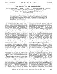
Figure 2: Functions f (±) (a) and g (±) (b).<br />
10<br />
8<br />
6<br />
4<br />
2<br />
0<br />
−2<br />
−4<br />
−6<br />
−8<br />
60<br />
g (−)<br />
g (+)<br />
−10<br />
−5 −4 −3 −2 −1 0<br />
E<br />
1 2 3 4 5<br />
The steady state Green functions may be conveniently written as<br />
ˆg R(A) = g R(A) ˆτ3 + f R(A) iˆτ2,<br />
simplify<strong>in</strong>g <strong>the</strong> equation to<br />
⎛<br />
⎝E + <br />
iηjg R(A)<br />
⎞<br />
⎠ = g R(A)<br />
⎛<br />
⎝|∆| + <br />
iηjf R(A)<br />
⎞<br />
⎠,<br />
f R(A)<br />
2<br />
j=2<br />
j<br />
which has <strong>the</strong> solution<br />
g R(A) E ± iγ<br />
2 = ± <br />
(E ± iγ) 2 − (|∆| ± iδ) 2 ×<br />
<br />
1, |E| < |∆|<br />
sgn(E), |E| > |∆|<br />
f R(A)<br />
|∆| ± iδ<br />
2 = ± <br />
(E ± iγ) 2 − (|∆| ± iδ) 2 ×<br />
<br />
1, |E| < |∆|<br />
sgn(E), |E| > |∆|<br />
2<br />
j=2<br />
(b)<br />
j<br />
60<br />
−60<br />
,<br />
, (21)<br />
where γ = R(A)<br />
j ηjgj and δ = R(A)<br />
j ηjfj . In <strong>the</strong> tunnel<strong>in</strong>g limit η ≪ ∆,<br />
<strong>the</strong>refore we neglect <strong>the</strong> exact forms of γ and δ and <strong>in</strong>stead use a constant<br />
γ = δ = 10−4 <strong>in</strong> <strong>the</strong> numerical calculations. We also def<strong>in</strong>e<br />
g (−) = Re g R = 1<br />
2 (gR − g A ), g (+) = Im g R = 1<br />
2i (gR + g A ),<br />
f (−) = Re f R = 1<br />
2 (fR − f A ), f (+) = Im f R = 1<br />
2i (fR + f A ). (22)<br />
These are plotted <strong>in</strong> Fig. 2. For energies <strong>in</strong>side <strong>the</strong> energy gap g (−) and f (−)<br />
are of <strong>the</strong> order of γ. The same applies for g (+) and f (+) outside <strong>the</strong> gap. The<br />
normalized superconduct<strong>in</strong>g density of states is just g (−) . These functions are<br />
extensively used below.<br />
11
3.3 Order parameter and observables<br />
The magnitude of <strong>the</strong> order parameter <strong>in</strong> <strong>the</strong> <strong>nonequilibrium</strong> Keldysh formalism<br />
is given by [6]<br />
|∆|<br />
λ =<br />
EC<br />
dE<br />
−EC 8 Tr (ˆτ1 − iˆτ2) ˆg K EC<br />
dE<br />
=<br />
−EC 4 fK , (23)<br />
where EC is <strong>the</strong> BCS cutoff energy. Insert<strong>in</strong>g f K for our <strong>SISIS</strong> system explicitely<br />
yields<br />
|∆| = λ<br />
EC <br />
dE fL2f<br />
2 −EC<br />
(−)<br />
E<br />
<br />
(+)<br />
− ifT2f<br />
E = λ<br />
EC<br />
2 −EC<br />
dEfL2f (−)<br />
E , (24)<br />
where <strong>the</strong> last equality follows because <strong>the</strong> magnitude of <strong>the</strong> order parameter<br />
is real. Because f (−) <strong>in</strong> <strong>the</strong> <strong>in</strong>tegrand depends on <strong>the</strong> magnitude of <strong>the</strong> order<br />
parameter, this is a self-consistency equation.<br />
As shown <strong>in</strong> <strong>the</strong> previous subsection, gR(A) = −¯g R(A) <strong>in</strong> a stationary <strong>nonequilibrium</strong><br />
state. This is equivalent to a particle-hole symmetry <strong>in</strong> <strong>the</strong> quasiclassical<br />
approximation, i.e., <strong>the</strong>re are always as many particle excitations as <strong>the</strong>re are<br />
hole excitations. Therefore <strong>the</strong> net charge density N is unchanged after a transition<br />
to a superconduct<strong>in</strong>g state and <strong>the</strong> chemical potential of a Cooper pair (µ)<br />
is <strong>the</strong> same as <strong>the</strong> chemical potential of an excited electron (eϕ). However, this<br />
equilibrium may be broken by charged perturbations, e.g., electron <strong>in</strong>jection,<br />
or conversion of normal current to supercurrent near an <strong>in</strong>terface. This leads<br />
to a situation known as charge imbalance <strong>in</strong> which <strong>the</strong>re are differ<strong>in</strong>g amounts<br />
of electrons and holes on opposite sides of <strong>the</strong> Fermi level. To compensate this<br />
effect <strong>the</strong> chemical potential of <strong>the</strong> excitations must be adjusted <strong>in</strong> order to<br />
ma<strong>in</strong>ta<strong>in</strong> overall electrical neutrality. The charge density is given by [9]<br />
<br />
dE<br />
N = N0 + 2ν(eϕ + µ) − ν<br />
2 Tr(ˆgK ), (25)<br />
where N0 is <strong>the</strong> charge density <strong>in</strong> normal state. Because N = N0, <strong>the</strong> chemical<br />
potential of <strong>the</strong> excitations is coupled to <strong>the</strong> chemical potential of <strong>the</strong> condensate<br />
through<br />
<br />
dE<br />
eϕ = −µ +<br />
4 Tr(ˆgK ). (26)<br />
The net current flow<strong>in</strong>g <strong>in</strong>to an island is given by <strong>the</strong> time derivative of <strong>the</strong> total<br />
charge, which leads to [8]<br />
<br />
dE<br />
I = ieνΩ<br />
4 Tr(ˆτ3 ÎK T ). (27)<br />
Here we have <strong>in</strong>cluded only <strong>the</strong> tunnel<strong>in</strong>g part of <strong>the</strong> collision <strong>in</strong>tegral, because<br />
elastic and <strong>in</strong>elastic processes conserve <strong>the</strong> particle number. In <strong>the</strong> absence of<br />
a potential difference this results <strong>in</strong> an equation for <strong>the</strong> supercurrent. For a<br />
f<strong>in</strong>ite supercurrent to appear, a phase gradient must exist across <strong>the</strong> junction<br />
accord<strong>in</strong>g to <strong>the</strong> dc <strong>Josephson</strong> relation. Therefore we will not put χ = 0 as<br />
earlier, ra<strong>the</strong>r we write <strong>the</strong> Green functions as<br />
ˆg R(A) = g R(A) ˆτ3 + f R(A) i (cosχˆτ2 + s<strong>in</strong> χˆτ1).<br />
12
We obta<strong>in</strong> for <strong>the</strong> expression of <strong>the</strong> supercurrent across junction 2-4<br />
I 2→4<br />
S = − 1<br />
<br />
dE fL2f<br />
2eR4<br />
(−)<br />
2 f (+) (−)<br />
4 + fL4f 4 f (+)<br />
<br />
2 s<strong>in</strong>(χ4 − χ2)<br />
<br />
+(fT2 − fT4) g (−)<br />
2 g(−) 4 + f(+) 2 f (+)<br />
<br />
4 cos(χ4 − χ2) . (28)<br />
Because also <strong>the</strong> supercurrent is conserved, I2→4 = −I2→5 . If a voltage is<br />
applied across <strong>the</strong> junction, Eq. (27) gives <strong>the</strong> quasiparticle current. It reads<br />
I 1→2 = − 1<br />
<br />
dE g<br />
4eR1<br />
(−)<br />
1,E+µ g(−)<br />
2,E (fL2 + fT2 − fL1 − fT1)<br />
+g (−)<br />
1,E−µ g(−)<br />
2,E (−fL2<br />
<br />
+ fT2 + fL1 − fT1) . (29)<br />
In a similar manner it is possible to obta<strong>in</strong> <strong>the</strong> <strong>the</strong> energy current, which is<br />
given by [8]<br />
<br />
dE<br />
Iε = −iνΩ<br />
4 Tr<br />
<br />
(E + eϕˆτ3) ÎK <br />
T . (30)<br />
These are <strong>the</strong> basic observables required to describe <strong>the</strong> behaviour of our system.<br />
4 Results<br />
4.1 Full nonequlibrium<br />
We beg<strong>in</strong> by present<strong>in</strong>g <strong>the</strong> calculated distribution function along with <strong>the</strong> order<br />
parameter and electric currents for <strong>the</strong> simplest, namely left-right symmetric<br />
case, where <strong>the</strong> tunnel junction resistances are <strong>the</strong> same and reservoirs 1 and<br />
3 are similar superconductors, i.e., R1 = R3 = R and |∆1| = |∆3| = |∆L|.<br />
Moreover, we assume <strong>the</strong> energy relaxation to be completely absent by sett<strong>in</strong>g<br />
<strong>the</strong> <strong>in</strong>elastic contributions to <strong>the</strong> self-energies <strong>in</strong> <strong>the</strong> previous section to zero.<br />
We fix <strong>the</strong> chemical potential of <strong>the</strong> island to zero and bias <strong>the</strong> structure with<br />
a voltage V . Current conservation forces <strong>the</strong> chemical potentials of reservoirs 1<br />
and 3 to µ1 = eV/2 and µ3 = −eV/2, respectively. This implies fL1 = fL3 = fL,<br />
. We also set <strong>the</strong> phase of <strong>the</strong><br />
fT1 = −fT3 = fT and g (−)<br />
E±µ1<br />
= g(−)<br />
E∓µ3<br />
= g(−)<br />
E±µ<br />
order parameter <strong>in</strong> <strong>the</strong> island to zero. This leads to ˆ H = −|∆|iˆτ2 simplify<strong>in</strong>g<br />
<strong>the</strong> k<strong>in</strong>etic equations (13) and (14) to<br />
with solutions<br />
g (−)<br />
E+µ (fL2 − fL − fT) + g (−)<br />
<br />
g (−)<br />
<br />
E+µ + g(−)<br />
E−µ<br />
g (−)<br />
2,E R−1 fT2<br />
fL2 = g(−)<br />
E+µ (fL + fT) + g (−)<br />
E−µ (fL2 − fL + fT) = 0, (31)<br />
= 4i|∆2|fT2f (+)<br />
2,E ν2e 2 Ω2, (32)<br />
g (−)<br />
E+µ + g(−)<br />
E−µ<br />
E−µ (fL − fT)<br />
,<br />
fT2 = 0. (33)<br />
This may also be written <strong>in</strong> terms of <strong>the</strong> full distribution functions as<br />
f2 = g(−)<br />
E+µ f1 + g (−)<br />
E−µ f3<br />
g (−)<br />
E+µ + g(−)<br />
E−µ<br />
13<br />
.
f 2<br />
1<br />
0.8<br />
0.6<br />
0.4<br />
0.2<br />
0<br />
T=0.1 T C<br />
E=−eV/2+∆ L<br />
−1 −0.8 −0.6 −0.4 −0.2 0 0.2 0.4 0.6 0.8 1<br />
E/∆ 0<br />
E=eV/2−∆ L<br />
v=0<br />
v=0.5<br />
v=1.5<br />
v=2.0<br />
v=2.5<br />
v=3.0<br />
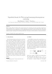
Figure 3: Nonequilibrium distribution function for <strong>the</strong> superconduct<strong>in</strong>g island<br />
at T = 0.1 TC. The cool<strong>in</strong>g effect reduc<strong>in</strong>g <strong>the</strong> number of excited quasiparticles<br />
as <strong>the</strong> voltage is <strong>in</strong>creased is evident. Here and below we denote v = eV/∆0<br />
and ∆0 = ∆L(T = 0).<br />
The full <strong>nonequilibrium</strong> distribution function for <strong>the</strong> superconduct<strong>in</strong>g island at<br />
a bath temperature, i.e., electron temperature <strong>in</strong> <strong>the</strong> large superconductors, of<br />
T = 0.1 TC 2 for various bias voltages is shown <strong>in</strong> Fig. 3. Upon <strong>in</strong>creas<strong>in</strong>g <strong>the</strong><br />
voltage above eV = ∆L, <strong>the</strong> number of excited quasiparticles <strong>in</strong> <strong>the</strong> island is<br />
clearly decreased with respect to equilibrium. This can be <strong>in</strong>terpreted as a lower<br />
effective electron temperature. This cool<strong>in</strong>g effect <strong>in</strong> SINIS and <strong>SISIS</strong> structures<br />
and its applications have been reviewed <strong>in</strong> [5]. The shape of <strong>the</strong> distribution<br />
function can be qualitatively expla<strong>in</strong>ed with a simple semiconductor model for<br />
<strong>the</strong> tunnel<strong>in</strong>g of quasiparticles, which is depicted <strong>in</strong> Fig. 4. In <strong>the</strong> semiconductor<br />
model <strong>the</strong> superconductors are modelled as ord<strong>in</strong>ary semiconductors with<br />
BCS density of states and energy gaps of 2∆. The transitions between metals<br />
are all horizontal, i.e. <strong>the</strong>y occur at constant energy levels after adjust<strong>in</strong>g <strong>the</strong><br />
relative levels of <strong>the</strong> chemical potentials to account for <strong>the</strong> potential difference.<br />
This model also presumes <strong>the</strong> symmetry between states outside and <strong>in</strong>side <strong>the</strong><br />
Fermi surface and it is <strong>in</strong>adequate for deal<strong>in</strong>g with processes <strong>in</strong> which Cooper<br />
pairs tunnel between metals. The states above <strong>the</strong> Fermi level (E > 0) are<br />
depopulated because <strong>the</strong>re is no <strong>in</strong>jection of particles from <strong>the</strong> energy gap <strong>in</strong><br />
reservoir 3, but extraction to states above <strong>the</strong> gap <strong>in</strong> reservoir 1 is possible.<br />
The states below <strong>the</strong> Fermi level (E < 0) are overpopulated because <strong>in</strong>jection<br />
is possible but extraction to gap is not. This can also be seen as excited holes<br />
tunnel<strong>in</strong>g out of <strong>the</strong> island. Maximum cool<strong>in</strong>g effect is achieved with a voltage<br />
of eV = 2∆L. If <strong>the</strong> voltage is fur<strong>the</strong>r <strong>in</strong>creased, hole <strong>in</strong>jection from above<br />
2 Here and <strong>in</strong> <strong>the</strong> follow<strong>in</strong>g TC denotes <strong>the</strong> critical temperature of <strong>the</strong> leads, i.e. reservoirs<br />
1 and 3.<br />
14
Reservoir 1 Island 2 Reservoir 3<br />
000000000000<br />
111111111111<br />
000000000000<br />
111111111111<br />
000000000000<br />
111111111111<br />
000000000000<br />
111111111111<br />
000000000000<br />
111111111111<br />
000000000000<br />
111111111111<br />
000000000000<br />
111111111111<br />
000000000000<br />
111111111111<br />
000000000000<br />
111111111111<br />
000000000000<br />
111111111111<br />
000000000000<br />
111111111111<br />
000000000000<br />
111111111111<br />
000000000000<br />
111111111111<br />
000000000000<br />
111111111111<br />
000000000000<br />
111111111111<br />
000000000000<br />
111111111111<br />
000000000000<br />
111111111111<br />
000000000000<br />
111111111111<br />
000000000000<br />
111111111111<br />
000000000000<br />
111111111111<br />
000000000000<br />
111111111111<br />
000000000000<br />
111111111111<br />
000000000000<br />
111111111111<br />
000000000000<br />
111111111111<br />
000000000000<br />
111111111111<br />
000000000000<br />
111111111111<br />
000000000000<br />
111111111111<br />
000000000000<br />
111111111111<br />
000000000000<br />
111111111111<br />
000000000000<br />
111111111111<br />
000000000000<br />
111111111111<br />
000000000000<br />
111111111111<br />
000000000000<br />
111111111111<br />
000000000000<br />
111111111111<br />
000000000000<br />
111111111111<br />
000000000000<br />
111111111111<br />
000000000000<br />
111111111111<br />
000000000000<br />
111111111111<br />
∆1<br />
000000000000<br />
111111111111<br />
000000000000<br />
111111111111<br />
000000000000<br />
111111111111<br />
000000000000<br />
111111111111<br />
000000000000<br />
111111111111<br />
000000000000<br />
111111111111<br />
000000000000<br />
111111111111<br />
000000000000<br />
111111111111<br />
000000000000<br />
111111111111<br />
000000000000<br />
111111111111<br />
000000000000<br />
111111111111<br />
000000000000<br />
111111111111<br />
000000000000<br />
111111111111<br />
000000000000<br />
111111111111<br />
000000000000<br />
111111111111<br />
e −<br />
eV<br />
2<br />
e −<br />
000000000000<br />
111111111111<br />
000000000000<br />
111111111111<br />
000000000000<br />
111111111111<br />
000000000000<br />
111111111111<br />
000000000000<br />
111111111111<br />
000000000000<br />
111111111111<br />
000000000000<br />
111111111111<br />
000000000000<br />
111111111111<br />
000000000000<br />
111111111111<br />
000000000000<br />
111111111111<br />
000000000000<br />
111111111111<br />
000000000000<br />
111111111111<br />
000000000000<br />
111111111111<br />
000000000000<br />
111111111111<br />
000000000000<br />
111111111111<br />
000000000000<br />
111111111111<br />
000000000000<br />
111111111111<br />
000000000000<br />
111111111111<br />
000000000000<br />
111111111111<br />
000000000000<br />
111111111111<br />
000000000000<br />
111111111111<br />
000000000000<br />
111111111111<br />
000000000000<br />
111111111111<br />
000000000000<br />
111111111111<br />
000000000000<br />
111111111111<br />
000000000000<br />
111111111111<br />
000000000000<br />
111111111111<br />
000000000000<br />
111111111111<br />
000000000000<br />
111111111111<br />
000000000000<br />
111111111111<br />
000000000000<br />
111111111111<br />
000000000000<br />
111111111111<br />
000000000000<br />
111111111111<br />
000000000000<br />
111111111111<br />
000000000000<br />
111111111111<br />
000000000000<br />
111111111111<br />
000000000000<br />
111111111111<br />
000000000000<br />
111111111111<br />
000000000000<br />
111111111111<br />
000000000000<br />
111111111111<br />
000000000000<br />
111111111111<br />
000000000000<br />
111111111111<br />
000000000000<br />
111111111111<br />
000000000000<br />
111111111111<br />
000000000000<br />
111111111111<br />
000000000000<br />
111111111111<br />
000000000000<br />
111111111111<br />
000000000000<br />
111111111111<br />
000000000000<br />
111111111111<br />
000000000000<br />
111111111111<br />
000000000000<br />
111111111111<br />
000000000000<br />
111111111111<br />
000000000000<br />
111111111111<br />
000000000000<br />
111111111111<br />
000000000000<br />
111111111111<br />
000000000000<br />
111111111111<br />
000000000000<br />
111111111111<br />
000000000000<br />
111111111111<br />
000000000000<br />
111111111111<br />
000000000000<br />
111111111111<br />
000000000000<br />
111111111111<br />
000000000000<br />
111111111111<br />
000000000000<br />
111111111111<br />
000000000000<br />
111111111111<br />
000000000000<br />
111111111111<br />
000000000000<br />
111111111111<br />
000000000000<br />
111111111111<br />
000000000000<br />
111111111111<br />
h +<br />
eV<br />
2<br />
h +<br />
000000000000<br />
111111111111<br />
000000000000<br />
111111111111<br />
000000000000<br />
111111111111<br />
000000000000<br />
111111111111<br />
000000000000<br />
111111111111<br />
000000000000<br />
111111111111<br />
000000000000<br />
111111111111<br />
000000000000<br />
111111111111<br />
000000000000<br />
111111111111<br />
000000000000<br />
111111111111<br />
000000000000<br />
111111111111<br />
000000000000<br />
111111111111<br />
000000000000<br />
111111111111<br />
000000000000<br />
111111111111<br />
000000000000<br />
111111111111<br />
∆3<br />
000000000000<br />
111111111111<br />
000000000000<br />
111111111111<br />
000000000000<br />
111111111111<br />
000000000000<br />
111111111111<br />
000000000000<br />
111111111111<br />
000000000000<br />
111111111111<br />
000000000000<br />
111111111111<br />
000000000000<br />
111111111111<br />
000000000000<br />
111111111111<br />
000000000000<br />
111111111111<br />
000000000000<br />
111111111111<br />
000000000000<br />
111111111111<br />
000000000000<br />
111111111111<br />
000000000000<br />
111111111111<br />
000000000000<br />
111111111111<br />
000000000000<br />
111111111111<br />
000000000000<br />
111111111111<br />
000000000000<br />
111111111111<br />
000000000000<br />
111111111111<br />
000000000000<br />
111111111111<br />
000000000000<br />
111111111111<br />
000000000000<br />
111111111111<br />
000000000000<br />
111111111111<br />
000000000000<br />
111111111111<br />
000000000000<br />
111111111111<br />
000000000000<br />
111111111111<br />
000000000000<br />
111111111111<br />
000000000000<br />
111111111111<br />
000000000000<br />
111111111111<br />
000000000000<br />
111111111111<br />
000000000000<br />
111111111111<br />
000000000000<br />
111111111111<br />
000000000000<br />
111111111111<br />
000000000000<br />
111111111111<br />
000000000000<br />
111111111111<br />
000000000000<br />
111111111111<br />
000000000000<br />
111111111111<br />
000000000000<br />
111111111111<br />
Figure 4: A semiconductor model for <strong>the</strong> tunnel<strong>in</strong>g of quasiparticles <strong>in</strong> <strong>the</strong> case<br />
eV > 2∆L. The dashed l<strong>in</strong>es represent <strong>the</strong> Fermi level <strong>in</strong> each part. The shape<br />
of <strong>the</strong> distribution <strong>in</strong> <strong>the</strong> middle electrode can be understood by not<strong>in</strong>g that <strong>the</strong><br />
tunnel<strong>in</strong>g of electrons (e − ) or holes (h + ) to <strong>the</strong> energy gap is forbidden. The<br />
divergence of <strong>the</strong> BCS density of states enhances <strong>the</strong> tunnel<strong>in</strong>g near gap edges<br />
because <strong>the</strong> quasiparticles have more available states to tunnel to. The electric<br />
current through <strong>the</strong> <strong>SISIS</strong> control l<strong>in</strong>e flows from left to right.<br />
<strong>the</strong> gap and particle <strong>in</strong>jection from below <strong>the</strong> gap <strong>in</strong> reservoirs 1 and 3, respectively,<br />
becomes possible. This leads to <strong>the</strong> peculiar shape of f2 for energies<br />
|E| < eV/2 − ∆L.<br />
In Fig. 5 <strong>the</strong> distribution function is plotted at higher bath temperatures for<br />
bias voltages eV/∆0 = 1 and eV/∆0 = 3. At higher temperatures <strong>the</strong> reservoirs<br />
have more excited quasiparticles above and below <strong>the</strong> gap, and <strong>the</strong> small notches<br />
at |E| = eV/2+∆L are a result of <strong>the</strong>ir <strong>in</strong>jection. The shape of <strong>the</strong> distribution<br />
for |E| < eV/2 − ∆L is reta<strong>in</strong>ed at high voltages and it should be noted that<br />
<strong>the</strong> edges stay very sharp regardless of <strong>the</strong> temperature.<br />
We also need to know <strong>the</strong> density of states <strong>in</strong> addition to <strong>the</strong>ir occupation<br />
with<strong>in</strong> <strong>the</strong> superconductor. This is given by g (−) , and we only need to f<strong>in</strong>d out<br />
<strong>the</strong> magnitude of <strong>the</strong> energy gap. This is given by Eq. (23). The <strong>in</strong>teraction<br />
constant λ can be excluded <strong>in</strong> favor of <strong>the</strong> zero-temperature order parameter<br />
by sett<strong>in</strong>g fL2 = fL2(T → 0) = sgn(E) and tak<strong>in</strong>g <strong>the</strong> limit γ → 0 <strong>in</strong> f (−) . We<br />
have<br />
EC<br />
|∆0|<br />
|∆0| =λ dE <br />
∆0 E2 − |∆0| 2 = λ|∆0|<br />
<br />
EC +<br />
ln<br />
E2 <br />
C − |∆0| 2<br />
|∆0|<br />
<br />
2EC<br />
≈λ|∆0| ln ,<br />
|∆0|<br />
15
f 2<br />
1<br />
0.8<br />
0.6<br />
0.4<br />
0.2<br />
0<br />
v=1.0<br />
E=−eV/2−∆ L<br />
E=eV/2+∆ L<br />
T=0.5 T C<br />
T=0.7 T C<br />
T=0.9 T C<br />
−3 −2 −1 0 1 2 3<br />
E/∆<br />
0<br />
(a) eV/∆0 = 1<br />
f 2<br />
1<br />
0.8<br />
0.6<br />
0.4<br />
0.2<br />
0<br />
v=3.0<br />
E=−eV/2−∆ L<br />
E=−eV/2+∆ L<br />
E=eV/2−∆ L<br />
T=0.5 T C<br />
T=0.7 T C<br />
T=0.9 T C<br />
E=eV/2+∆ L<br />
−3 −2 −1 0 1 2 3<br />
E/∆<br />
0<br />
(b) eV/∆0 = 3<br />
Figure 5: Nonequilibrium distribution function for <strong>the</strong> superconduct<strong>in</strong>g island<br />
at various bath temperatures for voltages eV/∆0 = 1 (a) and eV/∆0 = 3 (b).<br />
valid when EC ≫ |∆0|. Therefore<br />
λ =<br />
ln<br />
1<br />
2EC<br />
|∆0|<br />
For <strong>the</strong> numerics we adopt a method presented <strong>in</strong> [11]. We may approximate<br />
that fL2 ≈ 1 for energies above a certa<strong>in</strong> scale E∗ and thus get<br />
∗<br />
E<br />
1<br />
|∆| ≈ dE(fL2 − 1)f<br />
ln 0<br />
(−) <br />
EC<br />
|∆|<br />
+ dE <br />
∆ E2 − |∆| 2<br />
2EC<br />
|∆0|<br />
E ∗<br />
0<br />
.<br />
<br />
2EC<br />
|∆0|<br />
|∆|<br />
1<br />
= dE(fL2 − 1)f<br />
2EC<br />
ln 0<br />
|∆0|<br />
(−) <br />
2EC<br />
+ |∆| ln<br />
|∆|<br />
<br />
ln<br />
·<br />
<br />
2EC 2EC<br />
ln =ln +<br />
|∆0| |∆|<br />
1<br />
∗<br />
E<br />
dE(fL2 − 1)f<br />
|∆| 0<br />
(−)<br />
<br />
|∆|<br />
ln =<br />
|∆0|<br />
1<br />
∗<br />
E<br />
dE(fL2 − 1)f<br />
|∆| 0<br />
(−)<br />
<br />
|∆| =∆0 exp − 1<br />
∗<br />
E<br />
dE(1 − fL2)f<br />
|∆|<br />
(−)<br />
<br />
. (34)<br />
The magnitude of <strong>the</strong> order parameter of <strong>the</strong> island as a function of voltage at<br />
various bath temperatures is shown <strong>in</strong> Fig. 6(a). At T = 0.1 TC <strong>the</strong> odd-<strong>in</strong>-<br />
E part of <strong>the</strong> distribution is effectively unchanged outside <strong>the</strong> gap giv<strong>in</strong>g <strong>the</strong><br />
same result as for equilibrium. However, above eV = 2∆L <strong>the</strong> peculiar shape<br />
of <strong>the</strong> distribution makes it possible to have a lower value solution for <strong>the</strong> order<br />
parameter as well, giv<strong>in</strong>g rise to a hysteretic behavior with three solutions. Once<br />
voltage reaches eV = 2(∆2 + ∆L) <strong>the</strong> only possible solution is ∆2 = 0, because<br />
16
∆/∆ 0<br />
1.1<br />
1<br />
0.9<br />
0.8<br />
0.7<br />
0.6<br />
0.5<br />
eV=2(∆ L +∆ 2 )<br />
0.4<br />
0.3<br />
0.2<br />
0.1<br />
T=0.1 T<br />
C<br />
T=0.5 T<br />
C<br />
T=0.7 T<br />
C<br />
T=0.9 T<br />
C<br />
0<br />
0 0.5 1 1.5 2 2.5<br />
eV/∆<br />
0<br />
3 3.5 4 4.5 5<br />
(a)<br />
∆/∆ 0<br />
1.4<br />
1.2<br />
1<br />
0.8<br />
0.6<br />
0.4<br />
0.2<br />
T=0.7 T C<br />
eV=2(∆ 2 −∆ L )<br />
∆ 2 /∆ L =0.2<br />
∆ 2 /∆ L =0.5<br />
∆ 2 /∆ L =0.7<br />
∆ 2 /∆ L =1<br />
∆ 2 /∆ L =1.3<br />
0<br />
0 1 2 3 4<br />
eV/∆<br />
0<br />
Figure 6: The order parameter as a function of bias voltage at various bath<br />
temperatures (a) and ratios ∆2/∆L (b).<br />
<strong>the</strong> order parameter can never exceed its zero-temperature value, which would<br />
be needed <strong>in</strong> order to move <strong>the</strong> gap above eV/2 − ∆L (this stems from <strong>the</strong> fact<br />
that fL can never exceed 1). Equation (23) determ<strong>in</strong>es a situation <strong>in</strong> which <strong>the</strong><br />
free energy of <strong>the</strong> system is m<strong>in</strong>imized, i.e., dF/d∆ = 0. This condition can<br />
also describe a maximum <strong>in</strong> F [12]. Therefore, <strong>the</strong> multivalued behavior of <strong>the</strong><br />
order parameter can be <strong>in</strong>terpreted as different m<strong>in</strong>ima and maxima <strong>in</strong> <strong>the</strong> free<br />
energy. The values of <strong>the</strong> order parameter correspond<strong>in</strong>g to m<strong>in</strong>ima <strong>in</strong> <strong>the</strong> free<br />
energy are <strong>the</strong> solutions of Eq. (34) with a positive derivative with respect to<br />
∆<br />
<br />
d <br />
<br />
d∆<br />
∆=∆2<br />
<br />
|∆| − ∆0 exp<br />
<br />
− 1<br />
|∆|<br />
E ∗<br />
0<br />
(b)<br />
dE(1 − fL2)f (−)<br />
<br />
> 0.<br />
In this case <strong>the</strong> largest and smallest values represent m<strong>in</strong>ima and <strong>the</strong> middle<br />
value represents a maximum. If we <strong>in</strong>crease <strong>the</strong> voltage from zero, <strong>the</strong> system<br />
stays <strong>in</strong> <strong>the</strong> free-energy m<strong>in</strong>imum correspond<strong>in</strong>g to a superconduct<strong>in</strong>g state.<br />
Once we enter <strong>the</strong> hysteretic region, <strong>the</strong>rmal fluctuations may cause <strong>the</strong> system<br />
to jump to normal state, which is <strong>the</strong> o<strong>the</strong>r free-energy m<strong>in</strong>imum. In <strong>the</strong> absence<br />
of fluctuations, <strong>the</strong> system f<strong>in</strong>ally jumps to normal state at eV = 2(∆2 + ∆L).<br />
If we now proceed by decreas<strong>in</strong>g <strong>the</strong> voltage, <strong>the</strong> jump to <strong>the</strong> superconduct<strong>in</strong>g<br />
state may aga<strong>in</strong> occur somewhere <strong>in</strong> <strong>the</strong> hysteretic region. Once <strong>the</strong> voltage is<br />
decreased enough, only <strong>the</strong> superconduct<strong>in</strong>g state is possible.<br />
At higher bath temperatures <strong>the</strong> order parameter is <strong>in</strong>itially <strong>in</strong> its equilibrium<br />
value, but <strong>in</strong>creases with <strong>in</strong>creas<strong>in</strong>g voltage as <strong>the</strong> island cools. In Fig.<br />
6(b) <strong>the</strong> order parameter is shown for s<strong>in</strong>gle temperature of T = 0.7 TC but<br />
for different zero-temperature ratios ∆2/∆L = TC2/TC. For lower ratios, <strong>the</strong><br />
island is <strong>in</strong>itally <strong>in</strong> normal state because <strong>the</strong> bath temperature is above its critical<br />
temperature. Upon <strong>in</strong>creas<strong>in</strong>g <strong>the</strong> voltage, <strong>the</strong> island turns superconduct<strong>in</strong>g<br />
once <strong>the</strong> electron distribution is able to support an energy gap.<br />
F<strong>in</strong>ally, we calculate <strong>the</strong> supercurrent through <strong>the</strong> island us<strong>in</strong>g Eq. (28).<br />
In this case fT2 = fT4 = 0, so <strong>the</strong> latter term does not contribute, and <strong>the</strong><br />
17
eR 4 I/∆ 0<br />
1.8<br />
1.6<br />
1.4<br />
1.2<br />
1<br />
0.8<br />
0.6<br />
0.4<br />
0.2<br />
∆ 2 /∆ L =1<br />
T=0.1 T C<br />
T=0.5 T C<br />
T=0.7 T C<br />
T=0.9 T C<br />
0<br />
0 0.5 1 1.5 2 2.5 3 3.5 4 4.5 5 5.5<br />
eV/∆<br />
0<br />
(a)<br />
eR 4 I/∆ 0<br />
1.4<br />
1.2<br />
1<br />
0.8<br />
0.6<br />
0.4<br />
0.2<br />
∆ 2 /∆ L =0.7<br />
T=0.7 T C<br />
∆ 4 /∆ L =0.8<br />
∆ 4 /∆ L =0.9<br />
∆ 4 /∆ L =1.1<br />
0<br />
0 0.5 1 1.5 2 2.5 3 3.5 4 4.5 5<br />
eV/∆<br />
0<br />
Figure 7: The supercurrent as a function of bias voltage at different bath temperatures<br />
(a) and ratios ∆4/∆L (b). The ris<strong>in</strong>g and fall<strong>in</strong>g edges of <strong>the</strong> hysteresis<br />
have been marked with arrows. The small arrows <strong>in</strong> (b) <strong>in</strong>dicate voltages above<br />
which ∆2 > ∆4.<br />
expression for <strong>the</strong> supercurrent reduces to <strong>the</strong> form of <strong>the</strong> dc <strong>Josephson</strong> equation<br />
Eq. (1), with a critical current of<br />
IC = − 1<br />
<br />
dE fL2f<br />
2eR4<br />
(−)<br />
2 f (+) (−)<br />
4 + fL4f 4 f (+)<br />
<br />
2 . (35)<br />
For γ → 0, <strong>the</strong> first part of <strong>the</strong> <strong>in</strong>tegrand above is f<strong>in</strong>ite between ∆2 < E < ∆4<br />
and <strong>the</strong> second part is f<strong>in</strong>ite between ∆4 < E < ∆2. The critical current versus<br />
control voltage has been plotted <strong>in</strong> Fig. 7(a) for various bath temperatures.<br />
As can be seen, <strong>the</strong> supercurrent through <strong>the</strong> junction depends l<strong>in</strong>earily on <strong>the</strong><br />
magnitude of <strong>the</strong> order parameter <strong>in</strong> <strong>the</strong> island and <strong>the</strong> hysteretic behaviour of<br />
∆2 carries over to <strong>the</strong> supercurrent as well. Once <strong>the</strong> island jumps <strong>in</strong>to normal<br />
state, <strong>the</strong> supercurrent vanishes. In Fig. 7(b) <strong>the</strong> more <strong>in</strong>terest<strong>in</strong>g characteristics<br />
of <strong>the</strong> supercurrent are shown. For ∆2/∆L = 0.7 <strong>the</strong> non-hysteretic ris<strong>in</strong>g<br />
edge at low voltage gives a well-tunable supercurrent. The lower ratios ∆4/∆L<br />
also exhibit a current drop at voltage above which ∆2 > ∆4 where <strong>the</strong> second<br />
part of <strong>the</strong> <strong>in</strong>tegrand contributes. For higher ratios ∆2 is always smaller than<br />
∆4 and chang<strong>in</strong>g <strong>the</strong> ratio merely scales <strong>the</strong> magnitude of <strong>the</strong> supercurrent.<br />
The electric current through <strong>the</strong> <strong>SISIS</strong> control l<strong>in</strong>e may be calculated with Eq.<br />
(29). The result<strong>in</strong>g current is plotted <strong>in</strong> Fig. 8. It has <strong>the</strong> familiar form of<br />
a current through a voltage biased SIS-junction. At low bath temperatures<br />
with few excited quasiparticles <strong>the</strong>re is no current until <strong>the</strong> voltage exceeds<br />
eV = 2(∆L + ∆2) and <strong>the</strong> potential difference gives enough energy to create<br />
a particle on one side and a hole on <strong>the</strong> o<strong>the</strong>r side. At higher temperatures a<br />
small current exists below that due to tunnel<strong>in</strong>g of <strong>the</strong>rmally excited particles<br />
above <strong>the</strong> gap.<br />
18<br />
(b)
eR 1 I/∆ 0<br />
2.5<br />
2<br />
1.5<br />
1<br />
0.5<br />
T=0.1 T C<br />
T=0.7 T C<br />
T=0.9 T C<br />
0<br />
0 0.5 1 1.5 2 2.5 3 3.5 4 4.5 5<br />
eV/∆ 0<br />
eV=2(∆ L +∆ 2 )<br />
Figure 8: The electric current through <strong>the</strong> <strong>SISIS</strong> control l<strong>in</strong>e as a function of<br />
bias voltage.<br />
4.2 Relaxation-time approximation<br />
The quasiparticles enter<strong>in</strong>g <strong>the</strong> island tend to relax towards energy equilibrium<br />
as discussed <strong>in</strong> Subs. 2.1.2. This is achieved via <strong>in</strong>elastic collisions with impurities,<br />
lattice vibrations (phonons) and o<strong>the</strong>r electrons. At low temperatures <strong>the</strong><br />
most relevant scatter<strong>in</strong>g mechanism is electron-electron scatter<strong>in</strong>g. The simplest<br />
method to <strong>in</strong>clude <strong>the</strong> energy relaxation of <strong>the</strong> <strong>in</strong>jected particles is <strong>the</strong><br />
relaxation-time approach. Typically one compares <strong>the</strong> <strong>in</strong>teraction times measured<br />
from experiments to some characteristic scale of <strong>the</strong> problem. We assume<br />
that <strong>the</strong> distribution function has relaxed to <strong>the</strong> form<br />
f(E) = f 0 (E) + δf(E),<br />
where f0 is a Fermi function and δf is a small deviation from equilibrium.<br />
Therefore we may expand <strong>the</strong> collision <strong>in</strong>tegral as<br />
J (ee)<br />
<br />
1 [f] ≈<br />
δf ≡ − 1 0<br />
f − f , (36)<br />
∂J (ee)<br />
1<br />
∂f<br />
f=f 0<br />
where τee is <strong>the</strong> electron-electron scatter<strong>in</strong>g time which is assumed <strong>in</strong>dependent<br />
of <strong>the</strong> energy of <strong>the</strong> excitations. We fur<strong>the</strong>r assume that f 0 is <strong>the</strong> Fermi<br />
function <strong>in</strong> quasiequilibrium, i.e., steady state where electric and energy currents<br />
are conserved. These def<strong>in</strong>e <strong>the</strong> chemical potential and temperature of<br />
<strong>the</strong> quasiequilibrium, respectively, and are given by Eqs. (27) and (30). Insert<strong>in</strong>g<br />
<strong>the</strong>se <strong>in</strong>to k<strong>in</strong>etic equations yields <strong>the</strong> solution, presented <strong>in</strong> terms of <strong>the</strong><br />
19<br />
τee
f 2<br />
1<br />
0.8<br />
0.6<br />
0.4<br />
0.2<br />
0<br />
v=1.0 T=0.7 T C<br />
E=−∆ 2<br />
E=∆ 2<br />
Γτ ee =10 5<br />
Γτ ee =100<br />
Γτ ee =1<br />
Γτ ee =0.01<br />
−3 −2 −1 0 1 2 3<br />
E/∆<br />
0<br />
(a) eV/∆0 = 1<br />
f 2<br />
1<br />
0.8<br />
0.6<br />
0.4<br />
0.2<br />
0<br />
v=3.0 T=0.7 T C<br />
E=−∆ 2<br />
E=∆ 2<br />
Γτ ee =10 5<br />
Γτ ee =100<br />
Γτ ee =1<br />
Γτ ee =0.01<br />
−3 −2 −1 0 1 2 3<br />
E/∆<br />
0<br />
(b) eV/∆0 = 3<br />
Figure 9: Nonequilibrium distribution function for <strong>the</strong> superconduct<strong>in</strong>g island<br />
for various values of Γτee and voltages eV/∆0 = 1 (a) and eV/∆0 = 3 (b).<br />
full distribution functions,<br />
f2 =<br />
g (−)<br />
E+µ f1 + g (−)<br />
E−µ f3 +<br />
<br />
e2 <br />
ν2Ω2R/ g (−)<br />
g (−)<br />
E+µ + g(−)<br />
E−µ + e2ν2Ω2R/ 2,E τee<br />
<br />
g (−)<br />
2,E τee<br />
<br />
f 0 2<br />
. (37)<br />
The strength of <strong>the</strong> relaxation may be adjusted by vary<strong>in</strong>g <strong>the</strong> dimensionless<br />
parameter (Γτee) −1 ≡ e 2 ν2Ω2R/τee, where Γ is <strong>the</strong> tunnel<strong>in</strong>g <strong>in</strong>jection rate <strong>in</strong>to<br />
<strong>the</strong> island. The full distribution function for various strengths of <strong>the</strong> relaxation<br />
is shown <strong>in</strong> Fig. 9. As Γτee → ∞, <strong>the</strong> full <strong>nonequilibrium</strong> is reta<strong>in</strong>ed. The<br />
limit Γτee → 0 corresponds to quasiequilibrium, where f2 → f 0 2. The density of<br />
states for <strong>the</strong> island appear<strong>in</strong>g <strong>in</strong> Eq. (37) enhances <strong>the</strong> relaxation <strong>in</strong>side <strong>the</strong><br />
energy gap and creates sharp drops at |E| = ∆2.<br />
The effect of energy relaxation to <strong>the</strong> magnitude of <strong>the</strong> order parameter<br />
and supercurrent is shown <strong>in</strong> Fig. 10. With large values of Γτee no changes<br />
with respect to <strong>the</strong> full <strong>nonequilibrium</strong> can be seen. This is because <strong>the</strong> part of<br />
<strong>the</strong> distribution function affect<strong>in</strong>g <strong>the</strong> magnitude of <strong>the</strong> order parameter, i.e.,<br />
outside <strong>the</strong> gap, is mostly unchanged. The ehancement of <strong>the</strong> order parameter<br />
is suppressed with Γτee = 1 and vanishes completely when Γτee = 0.01. Also<br />
<strong>the</strong> hysteretic behaviour is lost <strong>in</strong> that limit.<br />
4.3 Collision <strong>in</strong>tegral<br />
The more accurate method to <strong>in</strong>clude <strong>the</strong> energy relaxation is to use <strong>the</strong> full<br />
electron-electron collision <strong>in</strong>tegrals. Here we use <strong>the</strong> collision <strong>in</strong>tegral for <strong>the</strong><br />
simplest form of electron-electron <strong>in</strong>teraction, namely po<strong>in</strong>t <strong>in</strong>teraction. If a<br />
superconductor is devoid of all impurities, <strong>the</strong> potential of a distant electron<br />
is completely screened by all o<strong>the</strong>r electrons. Therefore <strong>the</strong> potential may be<br />
20
∆/∆ 0<br />
1<br />
T=0.7 T<br />
C<br />
0.8<br />
0.6<br />
0.4<br />
0.2<br />
Γτ ee =10 5<br />
Γτ ee =100<br />
Γτ ee =1<br />
Γτ ee =0.01<br />
0<br />
0 0.5 1 1.5 2 2.5 3 3.5 4 4.5 5<br />
eV/∆<br />
0<br />
(a) Order parameter<br />
eR 4 I/∆ 0<br />
1.4<br />
1.2<br />
1<br />
0.8<br />
0.6<br />
0.4<br />
0.2<br />
Γτ ee =10 5<br />
Γτ ee =100<br />
Γτ ee =1<br />
Γτ ee =0.01<br />
0<br />
0 0.5 1 1.5 2 2.5 3 3.5 4 4.5 5<br />
eV/∆<br />
0<br />
(b) Supercurrent<br />
Figure 10: The magnitude of <strong>the</strong> order parameter (a) and supercurrent (b) for<br />
various values of Γτee at T = 0.7TC. Here all <strong>the</strong> superconductors were assumed<br />
similar, i.e., ∆2/∆L = ∆4/∆L = 1. The curves for Γτee = 10 5 and Γτee = 100<br />
co<strong>in</strong>cide.<br />
modelled with a delta function V (r) = V δ(r) and <strong>the</strong> collision <strong>in</strong>tegral is [9]<br />
J (ee)<br />
1 =4λ2 ee π<br />
pFvF<br />
×<br />
<br />
dE1dE2<br />
<br />
g (−)<br />
E1 g(−) − f(−)<br />
E2 E1 f(−)<br />
<br />
g E2<br />
(−)<br />
E g(−)<br />
E3<br />
<br />
(1 − fE)fE1fE2fE3 − fE (1 − fE1)(1 − fE2) (1 − fE3)<br />
+ f(−)<br />
E f(−)<br />
<br />
E3<br />
<br />
, (38)<br />
where pF and vF are Fermi momentum and velocity, respectively, λee is <strong>the</strong><br />
electron-electron <strong>in</strong>teraction constant and energies satisfy <strong>the</strong> conservation law<br />
E = E1+E2+E3. We note that because of <strong>the</strong> terms g (−)<br />
E3<br />
and f(−)<br />
E3 multiply<strong>in</strong>g<br />
<strong>the</strong> kernel of <strong>the</strong> <strong>in</strong>tegral, J (ee)<br />
1 ≈ γ when |E3| < ∆ and <strong>the</strong>refore it has very<br />
little effect on excitations <strong>in</strong>side <strong>the</strong> gap. We also note that <strong>the</strong> relaxation is<br />
strongest for excitations at |E3| = ∆. This is <strong>in</strong> stark contrast to <strong>the</strong> assumed<br />
energy <strong>in</strong>dependent scatter<strong>in</strong>g time of <strong>the</strong> relaxation-time approximation. Moreover,<br />
<strong>the</strong> collision <strong>in</strong>tegral at a given energy is <strong>in</strong> general not proportional to<br />
<strong>the</strong> difference between <strong>the</strong> true distribution function and <strong>the</strong> quasiequilibrium<br />
function f 0 evaluated at <strong>the</strong> same energy. The collision <strong>in</strong>tegral vanishes for <strong>the</strong><br />
quasiequilibrium function however, as can be seen by <strong>in</strong>sert<strong>in</strong>g f = f 0 . This<br />
time it is not possible to solve f2 explicitly, ra<strong>the</strong>r we must solve <strong>the</strong> result<strong>in</strong>g<br />
self-consistent equation<br />
f2 =<br />
g (−)<br />
E+µ f1 + g (−)<br />
E−µ f3 +<br />
<br />
g (−)<br />
E+µ + g(−)<br />
E−µ<br />
e 2 ν2Ω2R/g (−)<br />
2,E<br />
<br />
J (ee)<br />
(39)<br />
by numerical methods. The strength of <strong>the</strong> relaxation can be adjusted by vary<strong>in</strong>g<br />
<strong>the</strong> parameter κ ≡ 4πλ 2 eee 2 ν2Ω2R/pFvF. The distribution function for<br />
various κ with T = 0.7 TC is shown <strong>in</strong> Fig. 11. With <strong>the</strong> proper collision <strong>in</strong>tegral<br />
<strong>the</strong> distribution at energies <strong>in</strong>side <strong>the</strong> gap is practically unaffected. At <strong>the</strong><br />
21
f 2<br />
1<br />
0.8<br />
0.6<br />
0.4<br />
0.2<br />
0<br />
T=0.7 T C<br />
v=1<br />
E=−∆ 2<br />
E=∆ 2<br />
κ=0<br />
κ=0.01<br />
κ=0.1<br />
κ=1<br />
−3 −2 −1 0 1 2 3<br />
E/∆<br />
0<br />
(a) eV/∆0 = 1<br />
f 2<br />
1<br />
0.8<br />
0.6<br />
0.4<br />
0.2<br />
T=0.7 T C<br />
v=3<br />
E=−∆ 2<br />
κ=0<br />
κ=0.01<br />
κ=0.1<br />
κ=1<br />
0<br />
E=∆<br />
2<br />
−5 −4 −3 −2 −1 0<br />
E/∆<br />
0<br />
1 2 3 4 5<br />
(b) eV/∆0 = 3<br />
Figure 11: The full distribution function for <strong>the</strong> island for different stregths of<br />
relaxation and voltages eV/∆0 = 1 (a) and eV/∆0 = 3 (b). Only quasiparticles<br />
with energies outside <strong>the</strong> energy gap ∆2 are affected.<br />
lower voltage <strong>the</strong> island stays <strong>in</strong> <strong>the</strong> superconduct<strong>in</strong>g state with f<strong>in</strong>ite energy<br />
gap even with very high relaxation, and <strong>the</strong> quasiequilibrium limit cannot be<br />
reached. At <strong>the</strong> higher voltage <strong>the</strong> difference to relaxation-time approximation<br />
is most notable for small values of κ or (Γτee) −1 . Once <strong>the</strong> strength of <strong>the</strong><br />
relaxation is <strong>in</strong>creased, <strong>the</strong> gap goes to zero and <strong>the</strong> difference is lost. The<br />
order parameter and supercurrent for various values of κ are shown <strong>in</strong> Fig. 12.<br />
The magnitude of <strong>the</strong> order parameter is hysteretic even with strong relaxation<br />
contrary to <strong>the</strong> behaviour <strong>in</strong> <strong>the</strong> quasiequilibrium limit, where <strong>the</strong> hysteretic<br />
behaviour vanished.<br />
4.4 Asymmetric structure<br />
Let us now exam<strong>in</strong>e an asymmetric situation, where R1 = R3 or ∆1 = ∆3. By<br />
solv<strong>in</strong>g Eqs. (13) and (14) with J (<strong>in</strong>el)<br />
1 = J (<strong>in</strong>el)<br />
2 = 0 we obta<strong>in</strong> quite lengthy<br />
expressions for <strong>the</strong> odd and even parts of <strong>the</strong> distribution function<br />
DfL2 =4e 2 f (+)<br />
<br />
2 ν2Ω2|∆2| G1 (fL1 − fT1)g (−)<br />
1,E−µ1 + (fL1 + fT1)g (−)<br />
<br />
+ 1,E+µ1<br />
<br />
<br />
G3<br />
− g (−)<br />
<br />
2,E<br />
<br />
+G3<br />
DfT2 = − g (−)<br />
<br />
+G3<br />
(fL3 − fT3)g (−)<br />
3,E−µ3 + (fL3 + fT3)g (−)<br />
3,E+µ3<br />
2,E<br />
G1<br />
<br />
2fL1G1g (−)<br />
1,E−µ1 + (fL1 + fL3 + fT1 − fT3)G3g (−)<br />
3,E−µ3<br />
2fL3G3g (−)<br />
3,E−µ3 + (fL1 + fL3 − fT1 + fT3)G1g (−)<br />
1,E−µ1<br />
G1<br />
<br />
<br />
g (−)<br />
3,E+µ3<br />
<br />
2fT1G1g (−)<br />
1,E−µ1 + (fL1 − fL3 + fT1 + fT3) G3g (−)<br />
3,E−µ3<br />
<br />
2fT3G3g (−)<br />
3,E−µ3 + (−fL1 + fL3 + fT1 + fT3)G1g (−)<br />
1,E−µ1<br />
22<br />
g (−)<br />
1,E+µ1<br />
<br />
,<br />
<br />
g (−)<br />
1,E+µ1<br />
<br />
g (−)<br />
3,E+µ3<br />
(40)<br />
<br />
,
∆/∆ 0<br />
1<br />
0.8<br />
0.6<br />
0.4<br />
T=0.7 T C<br />
0.2<br />
κ=0<br />
κ=0.01<br />
κ=0.1<br />
κ=1<br />
0<br />
0 1 2<br />
eV/∆<br />
0<br />
3 4<br />
(a) Order parameter<br />
eR 4 I/∆ 0<br />
1.2<br />
1<br />
0.8<br />
0.6<br />
0.4<br />
T=0.7 T C<br />
0.2<br />
κ=0<br />
κ=0.01<br />
κ=0.1<br />
κ=1<br />
0<br />
0 1 2<br />
eV/∆<br />
0<br />
3 4<br />
(b) Supercurrent<br />
Figure 12: The magnitude of <strong>the</strong> order parameter (a) and supercurrent (b) for<br />
various strength of <strong>the</strong> relaxation and T = 0.7TC. Aga<strong>in</strong> all <strong>the</strong> superconductors<br />
were assumed similar. The small notches <strong>in</strong> <strong>the</strong> supercurrent with κ = 1 and<br />
κ = 0.1 are aga<strong>in</strong> <strong>the</strong> result of different parts of <strong>the</strong> <strong>in</strong>tegrand <strong>in</strong> Eq. (28) be<strong>in</strong>g<br />
f<strong>in</strong>ite.<br />
where<br />
D =4e 2 f (+)<br />
<br />
2 ν2Ω2|∆2| G1 g (−)<br />
<br />
+ g(−) + G3 g 1,E−µ1 1,E+µ1<br />
(−)<br />
3,E−µ3<br />
<br />
G1g (−)<br />
<br />
(−)<br />
+ G3g G1g 1,E−µ1 3,E−µ3<br />
(−)<br />
<br />
(−)<br />
+ G3g ,<br />
1,E+µ1 3,E+µ3<br />
− 2g (−)<br />
2,E<br />
+ g(−)<br />
3,E+µ3<br />
and Gi = 1/Ri are <strong>the</strong> conductances of <strong>the</strong> tunnel contacts. The distribution<br />
functions depend on <strong>the</strong> volume, energy gap and normal state density of states<br />
at <strong>the</strong> Fermi level, but <strong>the</strong>se can be <strong>in</strong>cluded <strong>in</strong> dimensionless constants of <strong>the</strong><br />
type G/|∆|νΩe 2 . In <strong>the</strong> asymmetric case <strong>the</strong> potentials µ1 and µ3 must be<br />
chosen such that <strong>the</strong> electrical current is conserved. This implies <strong>the</strong> vanish<strong>in</strong>g<br />
of <strong>the</strong> total net current I <strong>in</strong>to <strong>the</strong> island <strong>in</strong> Eq. (27). The conservation of electric<br />
current also forces <strong>the</strong> imag<strong>in</strong>ary part <strong>in</strong> Eq. (24) to vanish regardless of fT.<br />
The current through <strong>the</strong> junction and <strong>the</strong>refore also <strong>the</strong> potentials depend on<br />
<strong>the</strong> order parameter of <strong>the</strong> island. S<strong>in</strong>ce <strong>the</strong> correct potentials are <strong>in</strong> turn needed<br />
for calculat<strong>in</strong>g <strong>the</strong> order parameter, <strong>the</strong> equations must be solved iteratively.<br />
However, at low temperatures and low bias voltages <strong>the</strong> order parameter stays<br />
reasonably close to ∆0, and we can get an idea of <strong>the</strong> behaviour of <strong>the</strong> potentials<br />
by choos<strong>in</strong>g <strong>the</strong> order parameter to be a constant. The potential of reservoir 1<br />
has been plotted <strong>in</strong> Fig. 13 for different degrees of asymmetry at eV/∆0 = 1<br />
with a fixed order parameter. At low bath temperature <strong>the</strong> current through<br />
<strong>the</strong> control l<strong>in</strong>e is very small and very high resistance or energy gap ratios are<br />
required <strong>in</strong> order to significantly change <strong>the</strong> potential from eV/2. At higher<br />
temperatures <strong>the</strong> <strong>the</strong>rmally excited quasiparticles are able to tunnel above <strong>the</strong><br />
gaps lead<strong>in</strong>g to a higher current and a larger effect to <strong>the</strong> potentials. In <strong>the</strong><br />
limit ∆1,2,3 → 0 <strong>the</strong> condition on current conservation results <strong>in</strong> <strong>the</strong> Kirchoff’s<br />
voltage law.<br />
The full distribution function at T = 0.7 TC1 has been plotted for various<br />
23
eµ 1 /∆ 0<br />
1<br />
0.9<br />
0.8<br />
0.7<br />
0.6<br />
0.5<br />
10 0<br />
v=1<br />
10 1<br />
R 1 /R 3<br />
(a) ∆1 = ∆3<br />
T=0.1 T C<br />
T=0.7 T C<br />
10 2<br />
eµ 1 /∆ 0<br />
1<br />
0.9<br />
0.8<br />
0.7<br />
0.6<br />
v=1<br />
T=0.1 T C<br />
0.5<br />
T=0.7 T<br />
C<br />
1 1.5 2 2.5 3 3.5<br />
∆ /∆<br />
1 3<br />
4 4.5 5 5.5 6<br />
(b) R1 = R3<br />
Figure 13: The potential µ1 as a function of <strong>the</strong> ratio of resistances (a) or order<br />
parameters (b). The order parameter of <strong>the</strong> island has been fixed at ∆2 = ∆1.<br />
In <strong>the</strong> asymmetric situation we have <strong>in</strong>troduced a slightly different notation<br />
with ∆0 = ∆1(T = 0) and TC = TC1. Also note <strong>the</strong> logarithmic scale <strong>in</strong> (a).<br />
zero-temperature ratios ∆3/∆1 with a voltage eV/∆0 = 2.0 and ratios R1/R3<br />
with a voltage eV/∆0 = 1.5 <strong>in</strong> Fig. 14. Qualitatively <strong>the</strong> distribution function<br />
takes a form that can be deduced from <strong>the</strong> simple model presented earlier. The<br />
small notches at |E| = |µi| + ∆i result from <strong>the</strong> <strong>in</strong>jection of <strong>the</strong>rmally excited<br />
quasiparticles above <strong>the</strong> gaps of <strong>the</strong> reservoirs. The larger peaks at |E| =<br />
|µi| − ∆i result from <strong>the</strong> <strong>in</strong>jection of quasiparticles below <strong>the</strong> gaps. From <strong>the</strong><br />
small notches we may also observe that <strong>the</strong> distribution is no longer symmetric<br />
around E = 0 because fT is f<strong>in</strong>ite and <strong>the</strong>re is charge imbalance.<br />
The order parameter and supercurrent for χ4 − χ2 = π/2 is shown <strong>in</strong> Fig.<br />
15. In <strong>the</strong> asymmetric structure <strong>the</strong> magnitude of <strong>the</strong> order parameter seems<br />
to take a value close to its value <strong>in</strong> <strong>the</strong> symmetric case with a voltage of eV =<br />
2 max(|µ1|, |µ3|). This is reasonable because <strong>the</strong> distribution function <strong>in</strong> <strong>the</strong><br />
region |E| > max(∆1 + |µ1|, ∆3 + |µ3|) is similar to <strong>the</strong> distribution <strong>in</strong> <strong>the</strong><br />
symmetric structure. The superconductivity is lost once |µ1| > ∆2 + ∆1 or<br />
|µ3| > ∆2 + ∆3. With high asymmetry ratios <strong>the</strong> potentials differ very much<br />
from ±eV/2 and supercondictivity is lost at a lower bias voltage compared to<br />
<strong>the</strong> symmetric structure. Also <strong>the</strong> hysteretic region is evident. Once <strong>the</strong> voltage<br />
is <strong>in</strong>creased over <strong>the</strong> hysteretic region, no solution to Eq. (24) toge<strong>the</strong>r with <strong>the</strong><br />
conservation of current can be found. This may lead to some time-dependent<br />
dynamic behaviour to which our formalism is unsuitable.<br />
Because fT is f<strong>in</strong>ite, also <strong>the</strong> latter part of Eq. (28) may contribute depend<strong>in</strong>g<br />
on <strong>the</strong> phase difference between <strong>the</strong> superconductors. Its magnitude can be<br />
<strong>in</strong>vestigated by sett<strong>in</strong>g <strong>the</strong> phase difference to zero. In this case <strong>the</strong> supercurrent<br />
is significantly smaller. The cos(∆χ) deviation from <strong>the</strong> dc <strong>Josephson</strong> relation<br />
is negligible, because it is at least three orders of magnitude smaller than <strong>the</strong><br />
product g (−)<br />
2 g(−)<br />
4 . This is illustrated <strong>in</strong> Fig. 16. The small magnitude of <strong>the</strong><br />
cos(∆χ) deviation results ei<strong>the</strong>r from <strong>the</strong> small values of fT2 or small values of<br />
24
eR 4 I/∆ 0<br />
f 2<br />
1.2<br />
T=0.7 T<br />
C<br />
1<br />
0.8<br />
0.6<br />
0.4<br />
0.2<br />
1<br />
0.8<br />
0.6<br />
0.4<br />
0.2<br />
0<br />
R 1 /R 3 =1.1<br />
R 1 /R 3 =2<br />
R 1 /R 3 =5<br />
−3 −2 −1 0 1 2 3<br />
E/∆<br />
0<br />
(a) ∆1 = ∆3<br />
f 2<br />
T=0.7 T<br />
C<br />
1<br />
0.8<br />
0.6<br />
0.4<br />
0.2<br />
0<br />
∆ 3 /∆ 1 =1.1<br />
∆ 3 /∆ 1 =2<br />
∆ 3 /∆ 1 =3<br />
−3 −2 −1 0 1 2 3<br />
E/∆<br />
0<br />
(b) R1 = R3<br />
Figure 14: The distribution function for different ratios R1/R3 at eV/∆0 = 1.5<br />
(a) and ∆3/∆1 (b) at eV/∆0 = 2.0. The arrows are located at energies −µ1−∆1,<br />
µ3 − ∆3, −µ1 + ∆1 and µ3 + ∆3 (from left to right). The correspond<strong>in</strong>g peaks<br />
can also be seen above <strong>the</strong> Fermi level at exactly opposite energies.<br />
R 1 /R 3 =1.1<br />
R 1 /R 3 =2<br />
R 1 /R 3 =5<br />
0<br />
0 0.5 1 1.5 2 2.5<br />
eV/∆<br />
0<br />
(a) ∆1 = ∆3<br />
1.2<br />
1<br />
0.8<br />
0.6<br />
0.4<br />
0.2<br />
0<br />
∆/∆ 0<br />
eR 4 I/∆ 0<br />
1.2<br />
1<br />
0.8<br />
0.6<br />
0.4<br />
0.2<br />
∆ 3 /∆ 1 =1.1<br />
∆ 3 /∆ 1 =2<br />
∆ 3 /∆ 1 =3<br />
0<br />
0 0.5 1 1.5 2 2.5 3 3.5 4 4.5 5<br />
eV/∆<br />
0<br />
0<br />
(b) R1 = R3<br />
Figure 15: The magnitude of <strong>the</strong> order parameter and supercurrent for different<br />
ratios R1/R3 (a) and ∆3/∆1 (b).<br />
25<br />
1.2<br />
1<br />
0.8<br />
0.6<br />
0.4<br />
0.2<br />
∆/∆ 0
eR 4 I/∆ 0<br />
x 10−3<br />
1<br />
χ −χ =0<br />
4 2<br />
0<br />
−1<br />
−2<br />
−3<br />
−4<br />
−5<br />
R 1 /R 3 =1.1<br />
R 1 /R 3 =2<br />
R 1 /R 3 =5<br />
−6<br />
0 0.5 1 1.5 2 2.5<br />
eV/∆<br />
0<br />
(a) Supercurrent<br />
eR 4 I/∆ 0<br />
x 10−7<br />
0.5<br />
0<br />
−0.5<br />
−1<br />
−1.5<br />
−2<br />
cos(χ) prefactor<br />
R 1 /R 3 =1.1<br />
R 1 /R 3 =2<br />
R 1 /R 3 =5<br />
−2.5<br />
0 0.5 1 1.5 2 2.5<br />
eV/∆<br />
0<br />
(b) Prefactor of cos(∆χ)<br />
Figure 16: The magnitude of <strong>the</strong> supercurrent for χ4 − χ2 = 0.<br />
f (+)<br />
2 f (+)<br />
4 . The latter may be <strong>in</strong>creased by smear<strong>in</strong>g out <strong>the</strong> density of states.<br />
This can be achieved by <strong>in</strong>troduc<strong>in</strong>g magnetic impurities to <strong>the</strong> sample which<br />
is addressed <strong>in</strong> <strong>the</strong> next subsection.<br />
In pr<strong>in</strong>ciple, <strong>the</strong> energy relaxation <strong>in</strong> <strong>the</strong> asymmetric case could be <strong>in</strong>cluded<br />
by solv<strong>in</strong>g <strong>the</strong> k<strong>in</strong>etic equations with <strong>the</strong> collision <strong>in</strong>tegrals (ei<strong>the</strong>r proper or<br />
approximated). However, we do not have <strong>the</strong> proper collision <strong>in</strong>tegrals for <strong>the</strong><br />
case of f<strong>in</strong>ite charge imbalance and <strong>the</strong>ir application would be computationally<br />
unwieldy, <strong>the</strong>refore we do not pursue <strong>the</strong> energy relaxation fur<strong>the</strong>r this time.<br />
4.4.1 Sp<strong>in</strong>-flip scatter<strong>in</strong>g<br />
If magnetic impurities are <strong>in</strong>troduced to <strong>the</strong> central island, <strong>the</strong> <strong>in</strong>jected electrons<br />
may <strong>in</strong>teract with <strong>the</strong>m and scatter. In sp<strong>in</strong>-flip scatter<strong>in</strong>g <strong>the</strong> <strong>in</strong>cident electron<br />
changes <strong>the</strong> direction of its sp<strong>in</strong> <strong>in</strong> <strong>the</strong> scatter<strong>in</strong>g event. The sp<strong>in</strong>-flip scatter<strong>in</strong>g<br />
smears out <strong>the</strong> edges <strong>in</strong> <strong>the</strong> quasiparticle density of states and creates available<br />
states also <strong>in</strong>side <strong>the</strong> gap. The self-energy of <strong>the</strong> sp<strong>in</strong>-flip scatter<strong>in</strong>g is [9]<br />
ˆΣS = i<br />
ˆτ3ˆg ˆτ3, (41)<br />
2τS<br />
where 1/τS ≡ γ is <strong>the</strong> sp<strong>in</strong>-flip rate. In this case <strong>the</strong> steady-state Usadel equation<br />
can be written [13]<br />
f R(A)<br />
2 E + iγf R(A)<br />
2 g R(A)<br />
2 = g R(A)<br />
2 |∆|. (42)<br />
The solution to this equation is presented with a slightly different notation <strong>in</strong><br />
[13]. Even with <strong>the</strong> additional states <strong>in</strong>side <strong>the</strong> gap, <strong>the</strong> prefactor to cos(∆χ)<br />
is still two orders of magnitude smaller than <strong>the</strong> complete supercurrent with<br />
χ4 − χ2 = 0 as can be seen from Fig. 17. We can conclude that fT2 is too<br />
small where <strong>the</strong> rest of <strong>the</strong> <strong>in</strong>tegrand is f<strong>in</strong>ite for <strong>the</strong> cos<strong>in</strong>e-part to contribute.<br />
Indeed, as can be seen from Fig. 14 fT2 is f<strong>in</strong>ite only near <strong>the</strong> small notches at<br />
energies much larger than <strong>the</strong> gap, whereas f (+)<br />
2 f (+)<br />
4 is sufficiently large only<br />
<strong>in</strong>side <strong>the</strong> gap irregardless of <strong>the</strong> magnitude of γ.<br />
26
eR 4 I/∆ 0<br />
1<br />
0<br />
−1<br />
−2<br />
−3<br />
x 10−4<br />
2<br />
−4<br />
0 0.5 1 1.5 2<br />
eV/∆<br />
0<br />
(a)<br />
I C<br />
cos(χ) prefactor<br />
× 10 −2<br />
eR 4 I/∆ 0<br />
x 10−4<br />
0.5<br />
0<br />
−0.5<br />
−1<br />
−1.5<br />
−2<br />
−2.5<br />
−3<br />
× 10 −2<br />
−3.5<br />
I<br />
C<br />
cos(χ) prefactor<br />
−4<br />
0 0.1 0.2<br />
γ<br />
0.3 0.4 0.5<br />
Figure 17: The magnitude of <strong>the</strong> supercurrent and prefactor of cos(∆χ) for<br />
χ4 − χ2 = 0 with a sp<strong>in</strong>-flip rate of γ = 0.0125 (a) and with various sp<strong>in</strong>-flip<br />
rates at eV/∆0 = 2 (b).<br />
5 Discussion<br />
We have studied <strong>the</strong> <strong>SISIS</strong> <strong>Josephson</strong> <strong>transistor</strong> <strong>in</strong> full <strong>nonequilibrium</strong> <strong>regime</strong><br />
with <strong>the</strong> quasiclassical Keldysh-Green function formalism. The equations derived<br />
here are mostly <strong>the</strong> same as <strong>in</strong> Ref. [8], with <strong>the</strong> exception of <strong>the</strong> expression<br />
for <strong>the</strong> supercurrent <strong>in</strong> Eq. (28) and <strong>the</strong> exact form of <strong>the</strong> Green functions <strong>in</strong><br />
a superconductor with tunnel junctions <strong>in</strong> Eq. (21). The results show that<br />
<strong>the</strong> self-consistent calculation of <strong>the</strong> superconduct<strong>in</strong>g order parameter is important,<br />
because its hysteretic behaviour <strong>in</strong> <strong>nonequilibrium</strong> prevents <strong>the</strong> use of this<br />
structure as a <strong>transistor</strong> with a large differential current ga<strong>in</strong>. The ris<strong>in</strong>g edge<br />
of <strong>the</strong> supercurrent with unequal energy gaps <strong>in</strong> Fig. 7(b) can still be utilized,<br />
as well as <strong>the</strong> non-hysteretic fall<strong>in</strong>g edge where ∆2 and ∆4 cross.<br />
Ano<strong>the</strong>r approach would be to probe <strong>the</strong> degree of <strong>nonequilibrium</strong> <strong>in</strong> <strong>the</strong><br />
superconduct<strong>in</strong>g island by measur<strong>in</strong>g <strong>the</strong> supercurrent flow<strong>in</strong>g through it. However,<br />
<strong>the</strong> deviations from <strong>the</strong> Fermi distribution are strongest <strong>in</strong>side <strong>the</strong> energy<br />
gap, whereas <strong>the</strong> supercurrent is only affected by <strong>the</strong> distribution outside <strong>the</strong><br />
gap. Only <strong>the</strong> chang<strong>in</strong>g magnitude of <strong>the</strong> order parameter and its effect to<br />
<strong>the</strong> supercurrent can produce observable characteristics that would enable us to<br />
extract <strong>in</strong>formation about <strong>the</strong> degree of <strong>nonequilibrium</strong>.<br />
The energy relaxation <strong>in</strong>side <strong>the</strong> energy gap with <strong>the</strong> proper collision <strong>in</strong>tegral<br />
is qualitatively very different from <strong>the</strong> relaxation-time approximation. As<br />
a result <strong>the</strong> quasiequilibrium limit is unreachable as long as <strong>the</strong> island is superconduct<strong>in</strong>g.<br />
Outside <strong>the</strong> gap <strong>the</strong>ir difference is much smaller. The magnitude<br />
of <strong>the</strong> order parameter and <strong>the</strong>refore also <strong>the</strong> supercurrent drop down to low<br />
values more quickly with <strong>the</strong> proper energy relaxation and most notably <strong>the</strong><br />
sharp characteristics of <strong>the</strong> supercurrent <strong>in</strong> <strong>the</strong> quasiequilibrium limit become<br />
hysteretic. To our knowledge this calculation has not been done before for<br />
superconductors.<br />
To fur<strong>the</strong>r pursue <strong>the</strong> study of this topic one could take <strong>in</strong>to account <strong>the</strong><br />
27<br />
(b)
operation of <strong>the</strong> <strong>Josephson</strong> junctions <strong>in</strong> <strong>the</strong> dissipative <strong>regime</strong>, which is required<br />
<strong>in</strong> order to calculate <strong>the</strong> real values of power and current ga<strong>in</strong>. The actual<br />
behaviour of <strong>the</strong> asymmetric system at large voltages can also present <strong>in</strong>terest<strong>in</strong>g<br />
results. The possibility of a supercurrent with a cos(∆χ) dependence <strong>in</strong> <strong>the</strong><br />
presence of a charge imbalance might warrant some additional study as well,<br />
and it might be realizable with a different structure.<br />
References<br />
[1] F. Giazotto, T. T. Heikkilä, F. Taddei, R. Fazio, J. P. Pekola, and F. Beltram.<br />
Phys. Rev. Lett., 92, 137001 (2004).<br />
[2] A. M. Sav<strong>in</strong>, J. P. Pekola, J. T. Flyktman, A. Anthore, and F. Giazotto.<br />
Appl. Phys. Lett., 84, 4179 (2004).<br />
[3] F. Giazotto and J. P. Pekola. J. Appl. Phys., 97, 023908 (2004).<br />
[4] M. T<strong>in</strong>kham. Introduction to superconductivity. Dover publications Inc.,<br />
M<strong>in</strong>eola, New York, 2nd edition (1996).<br />
[5] F. Giazotto, T. T. Heikkilä, A. Luukanen, A. M. Sav<strong>in</strong>, and J. P. Pekola.<br />
Rev. Mod. Phys., 78, 217 (2006).<br />
[6] J. Rammer and H. Smith. Rev. Mod. Phys, 58, 323 (1986).<br />
[7] W. Belzig, F. K. Wilhelm, C. Bruder, G. Schön, and A. D. Zaik<strong>in</strong>. Superlattices<br />
and Microstructures, 25, 1251 (1999).<br />
[8] J. Voutila<strong>in</strong>en, T. T. Heikkilä, and N. B. Kopn<strong>in</strong>. Phys. Rev. B, 72, 054505<br />
(2005).<br />
[9] N. B. Kopn<strong>in</strong>. Theory of <strong>nonequilibrium</strong> superconductivity. International<br />
series of monographs on physics. Oxford university press, Oxford (2001).<br />
[10] U. Eckern and A. Schmid. J. <strong>Low</strong> Temp. Phys., 45, 137 (1981).<br />
[11] T. T. Heikkilä. Simple model for <strong>nonequilibrium</strong> heat<strong>in</strong>g of a superconductor<br />
(2004). Unpublished.<br />
[12] D. R. Hesl<strong>in</strong>ga and T. M. Klapwijk. Phys. Rev. B, 47, 5157 (1993).<br />
[13] A. Anthore. Decoherence mechanisms <strong>in</strong> mesoscopic conductors. Ph.D.<br />
<strong>the</strong>sis, University of Paris (2003).<br />
[14] G.-L. Ingold and Y. V. Nazarov. S<strong>in</strong>gle charge tunnel<strong>in</strong>g, volume 294 of<br />
NATO ASI Series B: Physics, chapter 2, pages 21–107. Plenum Press, New<br />
York (1992).<br />
[15] T. T. Heikkilä. Private communication.<br />
[16] V. Ambegaokar and A. Baratoff. Phys. Rev. Lett., 10, 486 (1963).<br />
28
A Tunnel<strong>in</strong>g rate<br />
A standard way of calculat<strong>in</strong>g <strong>the</strong> tunnel<strong>in</strong>g rate through a junction is to apply<br />
perturbation <strong>the</strong>ory. The Hamiltonian of <strong>the</strong> system is written<br />
H = Hqp + HT, (43)<br />
where Hqp describes <strong>the</strong> quasiparticle dynamics and HT <strong>the</strong>ir tunnel<strong>in</strong>g through<br />
<strong>the</strong> junction. Written with <strong>the</strong> help of <strong>the</strong> creation and annihilation operators<br />
c † and c, <strong>the</strong> tunnel<strong>in</strong>g Hamiltonian has <strong>the</strong> form [4]<br />
HT = <br />
σkq<br />
Tkqc †<br />
kσ cqσ + Herm. conj., (44)<br />
where <strong>the</strong> subscript k refers to one metal and q to <strong>the</strong> o<strong>the</strong>r and T is a tunnel<strong>in</strong>g<br />
matrix element. Therefore <strong>the</strong> first part of <strong>the</strong> tunnel<strong>in</strong>g Hamiltonian transfers<br />
an electron from <strong>the</strong> first metal with wave vector k to <strong>the</strong> second with wave<br />
vector q, while <strong>the</strong> Hermitian conjugate does <strong>the</strong> opposite. If <strong>the</strong> tunnel<strong>in</strong>g<br />
Hamiltonian is small, we may apply Fermi’s Golden Rule, i.e., use <strong>the</strong> lead<strong>in</strong>g<br />
order approximation <strong>in</strong> <strong>the</strong> perturbation to calculate <strong>the</strong> tunnel<strong>in</strong>g rate (see for<br />
example [14]). Accord<strong>in</strong>g to it, <strong>the</strong> transition rate from some <strong>in</strong>itial state i to a<br />
f<strong>in</strong>al state f is given by<br />
Γf←i = 2π |〈f|HT |i〉| 2 δ(Ef − Ei). (45)<br />
To obta<strong>in</strong> <strong>the</strong> total tunnel<strong>in</strong>g rate from metal 1 to metal 2 we need to sum over<br />
all <strong>in</strong>itial states weighed with <strong>the</strong>ir probabilities and over all f<strong>in</strong>al states:<br />
Γ12(V ) = 2π <br />
pk |〈ǫq|HT |ǫk〉| 2 δ(ǫq − ǫk − eV ), (46)<br />
kq<br />
where pk is <strong>the</strong> probability of an <strong>in</strong>itial state and eV is <strong>the</strong> difference <strong>in</strong> chemical<br />
potentials. We note that <strong>the</strong> matrix element 〈ǫq|c †<br />
kσ cqσ|ǫk〉 is nonvanish<strong>in</strong>g only<br />
for <strong>in</strong>itial states that have a quasiparticle of wave vector k and sp<strong>in</strong> σ present and<br />
f<strong>in</strong>al states that have a state with wave vector q and sp<strong>in</strong> σ unoccupied. Now<br />
we may write <strong>the</strong> occupation probabilities with Fermi-functions and transform<br />
<strong>the</strong> sum to an <strong>in</strong>tegral<br />
∞<br />
Γ12(V ) =2π dǫkdǫqf 0 (ǫk)(1 − f 0 (ǫq)) <br />
|Tkq| 2 ν1(ǫk)ν2(ǫq)Ω1Ω2δ(ǫq − ǫk − eV )<br />
= 1<br />
e 2 RT<br />
−∞<br />
σkq<br />
∞<br />
dEf 0 (E)(1 − f 0 (E + eV ))<br />
−∞<br />
≈ eV<br />
e2 , (47)<br />
RT<br />
where we have <strong>in</strong>troduced <strong>the</strong> tunnel resistance RT ≡ (4πe 2 |T | 2 ν1ν2Ω1Ω2) −1<br />
and assumed that <strong>the</strong> densities of state are effectively constant <strong>in</strong> <strong>the</strong> range<br />
where <strong>the</strong> <strong>in</strong>tegrand is f<strong>in</strong>ite. We have fur<strong>the</strong>r assumed a tunnel<strong>in</strong>g probability<br />
T <strong>in</strong>dependent of <strong>the</strong> <strong>in</strong>itial or f<strong>in</strong>al states. The last approximation is valid at<br />
low temperatures. The total current through <strong>the</strong> junction is given by<br />
I(V ) = e (Γ12(V ) − Γ21(V )), (48)<br />
29
which results <strong>in</strong> <strong>the</strong> same expression as Eq. (29). For <strong>the</strong> tunnel<strong>in</strong>g rate from<br />
one <strong>in</strong>itial state (which also gives <strong>the</strong> lifetime of <strong>the</strong> state) we have [15]<br />
η12 = Γ12<br />
ν1Ω1eV = (4ν1e 2 Ω1RT) −1 , (49)<br />
which is also used <strong>in</strong> <strong>the</strong> tunnel<strong>in</strong>g self energy.<br />
B Ambegaokar-Baratoff formula for <strong>the</strong> critical<br />
current<br />
A formula for <strong>the</strong> critical current between two similar superconductors (same<br />
energy gaps) <strong>in</strong> equilibrium was derived by Ambegaokar and Baratoff <strong>in</strong> [16].<br />
The same formula can be derived analytically from Eq. (35) and we present<br />
it here for completeness. At zero bias voltage fL2 = fL4 = tanh(E/2T) and<br />
f (−)<br />
2 f (+)<br />
4<br />
IC = − 1<br />
eR<br />
= f(−) 4 f (+)<br />
2 = 1/4i(fR − fA )(fR + fA ) result<strong>in</strong>g <strong>in</strong><br />
∞ <br />
E 1 |∆|<br />
dE tanh<br />
2T 4i<br />
2<br />
(E + iγ) 2 |∆|<br />
−<br />
− |∆| 2 2<br />
(E − iγ) 2 − |∆| 2<br />
<br />
.<br />
−∞<br />
This has poles at zj = ±|∆| ±iγ and zj = 2iTπ 1<br />
2 + m , where m is an <strong>in</strong>teger.<br />
Integration along a contour around <strong>the</strong> poles <strong>in</strong> <strong>the</strong> upper half plane and <strong>the</strong><br />
use of residue <strong>the</strong>orem yields<br />
IC = 1<br />
⎧<br />
⎨<br />
π <br />
z<br />
<br />
Res tanh<br />
eR ⎩ 2 z=zj 2T<br />
<br />
|∆| 2<br />
(z + iγ) 2 |∆|<br />
−<br />
− |∆| 2 2<br />
(z − iγ) 2 − |∆| 2<br />
⎫ ⎬<br />
⎭ .<br />
j<br />
Calculat<strong>in</strong>g <strong>the</strong> residues and lett<strong>in</strong>g γ → 0 results <strong>in</strong><br />
IC = π|∆|<br />
2eR tanh<br />
which is <strong>the</strong> Ambegaokar-Baratoff-relation.<br />
30<br />
|∆|<br />
2T<br />
<br />
, (50)