Swarm Navigation in a Complex Environment - World Academy of ...

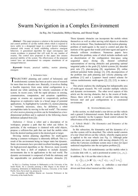
Abstract—This paper proposes a solution to the motion planning 

and control problem of car-like mobile robots which is required to 

move safely to a designated target in a priori known workspace 

cluttered with swarm of boids exhibiting collective emergent 

behaviors. A generalized algorithm for target convergence and 

swarm avoidance is proposed that will work for any number of 

swarms. The control laws proposed in this paper also ensures 

practical stability of the system. The effectiveness of the proposed 

control laws are demonstrated via computer simulations of an 

emergent behavior. 

Keywords—Swarm, practical stability, motion planning, 

emergent. 

I. INTRODUCTION 

RAJECTORY planning and control of holonomic and 

Tnonholonomic 

systems has been an active area of research 

for more than two decades now. Basically, it involves finding 

a feasible trajectory from some initial configuration to a 

desired one while satisfying the velocity constraints of the 

system. In recent years, with the rapid advances in sensing, 

communication, computation, and actuation capabilities, 

groups or swarms are expected to cooperatively perform 

dangerous or explorative tasks in a broad range of potential 

applications. As highlighted by Latombe [1], motion planning 

is “eminently necessary, since, by definition, a robot 

accomplishes tasks by moving in the real world”. The essence 

of robot motion planning problem can be formulated as a twodimensional 

problem and is captured in the following classic 

definition (adopted from [2]): 

Definition 1: Given a robot and a description of its 

workspace, propose a path that the robot can follow. In 

particular, if the workspace is cluttered with solid objects, 

propose a collision-free path that can lead the mobile robot 

from the desired starting point to the desired goal or target. 

Devising motion planning algorithms for multi-agents 

sharing a common workspace is inherently difficult. This is a 

result of the environment being no longer static but dynamic. 

Static environments have provided excellent breeding grounds 

for high-powered algorithms so far. However, more recently 

there has been a shift of emphasis to include dynamic 

environments due to its applications in the real world. The 

dynamic environment is composed of both the stationary and 

the unpredictable (or predictable) dynamic obstacles [3]. 

Jai Raj is a Teaching Assistant in Mathematics at the University of the 

South Pacific. He is currently pursuing a MSc Degree in the School of 

Computing, Information & Mathematical Sciences, University of the South 

Pacific, Suva, Fiji (e-mail: raj_j@usp.ac.fj). 

Jito Vanualailai and Bibhya Sharma are Associate Professors at the 

University of the South Pacific. 

World Academy of Science, Engineering and Technology 72 2012 

Swarm Navigation in a Complex Environment 

Jai Raj, Jito Vanualailai, Bibhya Sharma, and Shonal Singh 

1157 

These dynamic obstacles can incorporate the mobile robots 

themselves as well as other moving solid objects or obstacles 

in the environment. Thus, fundamental to the motion planning 

problem of multi-agents is the need to control and plan the 

motions of the agents that would yield inter-agent and agent to 

obstacle collision avoidances. Numerous papers have 

discussed this problem, some of which includes methods such 

as discretization of the configuration time-space using 

sequential space slicing [4], sheared cylindrical 

representations of moving obstacles and generating optimal 

tangential paths to the goals [5], hybrid systems [6], threaded 

petri nets [7], plan-merging [8], negotiations [9], online 

artificial potential fields strategy [1], [10], decomposition of 

the problem into path planning and velocity planning subproblems 

[11] and a Lyapunov based control scheme for 

various nonholonomic multi-agents [2], [3], [12], to name a 

few. 

This article explores the challenging but indispensable area 

of multi-agent research. We will consider multiple vehicles 

and dynamic environments. The other novel aspects of this 

article are the moving obstacles, that is, the swarm of boids. 

Hence, there will be a number of car-like robots moving 

between start and goal configurations in a constrained 

environment. 

II. SYSTEM MODELLING 

In this section, we shall model a rear driven car-like vehicle 

and a general 2-dimensional swarm. Both the models will be 

used to illustrate via the Lyapunov based control scheme the 

effectiveness of the system models. 

A. Vehicle Model - The Kinematics and Dynamics of the 

Car-like Robot 

In this subsection, the kinematics and the dynamics of a 

car-like system will be described. The vehicle model consists 

of a rear wheel driven car-like vehicle, whereby engine power 

is applied to the rear wheels (see Fig. 1). Although polar 

coordinates are more popular with moving obstacle [13], we 

utilize the Cartesian coordinate system since it does not inject 

undesired singularities into the navigation problem [2]. 

Definition 2: The k th nonholonomic car-like mobile robot is 

a circular disk with rv k and is positioned at center ( xvk, yv k) 

. 

In addition, the k th car-like robot is the set 

2 

2 2 

A = z , z ∈R : z − xv + z − yv ≤ rv , 

k { ( 1 2) ( 1 k) ( 2 k) k} 

for k { 1,..., m} , m , 

∈ ∈N where A k embodies a rear-wheel 

driven and front-wheel steered car-like vehicle.

Fig. 1 A rear wheel driven vehicle with front wheel steering and 

steering angle φ k . 

Inclusion of the dynamics will then be producing a 

trajectory in the state-space. Thus, if m k is the mass of the 

vehicle, k F the force along the axis of the vehicle, Γk the 

torque about a vertical axis at ( xvk, yv k) 

and I k the moment 

of inertia of the vehicle, then dynamic model of the vehicle is 

L ⎫ 

xv k = vk cosθk − wk 

sin θk, 

2 

⎪ 

⎪⎪ 

L 

yv k = vk sinθk + wk 

cos θk, 

2 ⎪ 

θk 

= wk, 

⎬ 

⎪ 

vk = σ k1: = Fk / mk, 

⎪ 

⎪⎪⎪ 

wk = σ k2: =Γk / Ik 

⎭ 

where the variable θ k gives the vehicles’s orientation with 

respect to the main axes, k v and w k are the translational and 

rotational velocities, respectively, while σ k1 

and k 2 

(1) 

σ are, 

respectively, the instantaneous translational and rotational 

accelerations. 

Referring to Fig. 1, to ensure that the entire vehicle safely 

steers past an obstacle, the planar vehicle will be enclosed by 

the smallest circle possible. L and l are, respectively, the 

length and width of the vehicle, then given the clearance 

parameters ε 1 and ε 2 , enclose the vehicle by a protective 

xv , yv , with radius 

circular region centered at ( ) 

k k 

( ε ) ( ε ) 

2 2 

1 2 

rv : = 2 + L + 2 + l /2. 

k 


1158 

Assumption 1: The instantaneous accelerations σ k1 

and σ k 2 

can move the car-like robot of A k to its designated target and 

attain the desired final orientation. 

B. A Two Dimensional Swarm Model 

Following the nomenclature of Reynolds [15], each 

member of the flock is denoted as a boid. We shall construct a 

model of a swarm with m individuals moving with the 

velocity of the swarm’s centroid. Following previous work 

such as those of [16] and [17], we consider the individuals as 

point masses. 

At time t ≥ 0 , let ( xbi( t) , ybi( t) ) , i = 1,..., n be the planar 

position of the i th individual, which we shall define as a 

point mass residing in a disk of radius rb i > 0, 

2 2 2 2 

{ ( 1 2) ( 1 ) ( 2 ) } 

B = z , z ∈R : z − xb + z − yb ≤ rb . (2) 

i i i i 

( ) ( ( ) ( ) ) 

At time t ≥ 0 , let vbi ( t) , wbi ( t) : = xb i t , yb i t be its 

instantaneous velocity of the i th point mass. Using the above 

notations, we thus have a system of first order ODE’s for the 

t = t ≥ : 

i th individual, assuming the initial conditions at 0 0 

( ) , 

() , 

( ) ( ) 

xb i = vbi t 

⎫ 

⎪ 

yb i = wbi t 

⎬ (3) 

⎪ 

xbi0 : = xbi t0 , ybi0 = ybi y0 

. ⎭ 

2 

2 

If gi ( x) : = ( vbi, wbi) 

∈Rand G( x) : = ( g1( x) ,..., gn( x) 

) ∈R 

, then our swarm system of m individuals is 

( ) ( ) 

x = G x , x = x t . 

(4) 

0 0 

Definition 3: System (4) is said to be 

(S1) practically stable if given ( λ , A) 

with 0 < λ < A , we 

have 

* () () 

* 

x0x λ 

− < implies that 

x t − x t < A, t ≥ t0for 

some t 0 ∈ R + ; 

(S2) uniformly practically stable if (S1) holds for every 

t 0 ∈ R + . 

The following comparison principle for practical stability is 

also adapted from [18] for system (4), where, 

K = { a∈C[ R+ , R+ ] : a( u) 

is strictly increasing in u and 

2 n 

a( u) →∞ as u →∞, S( ρ ) = { x∈R : 

* 

x− x < ρ} 

, and, 

2 n 

for any Lyapunov-like function V ∈ C ⎡ 

⎣R+ × R , R ⎤ + ⎦, 

V( t+ h, x+ hG( x) ) −V( 

t, x) 

+ 

DV( tx , ) : = limsup , 

+ 

h→0 

h 

for 

2n 

1 

( tx , ) ∈ R+ × R , noting that if V ∈ C [ R+ × R2 n, 

R + ] , then 

+ 

DV tx , V' tx , , V ' t, x = V t, x + V t, x G x . 

( ) = ( ) where ( ) ( ) ( ) ( ) 

t x 

n

Theorem 1: Lakshmikantham, Leela and Martynyuk [18]. 

Assume that 

1. λ and A are given such that 0 < λ < A ; 

2 n 

2. V ∈ C ⎡ 

⎣R+ × R , R ⎤ + ⎦ and V ( t, x ) is locally Lipschitzian 

in x ; 

* * 

3. for ( tx) ∈ R + × S( A) b1( x−x) ≤V( tx) ≤b2( x−x) , , , , 

2 

∈ and ( ) ( ( ) ) 

+ 

b1, b2 K DV tx , ≤ q tV , tx , , q∈C⎡ ⎣R+ , R ⎤ 

⎦; 

4. b2( λ ) < b1( A) 

holds. 

Then the practical stability properties of the scalar 

differential equation 

( ) ( ) ( ) 

z' t = q t, z , z t = z ≥ 0, 

0 0 

imply the corresponding practical stability properties of 

system (4). 

III. DEPLOYMENT OF THE LYAPUNOV-BASED 

CONTROL SCHEME 

The principal control objective of this section is to utilize 

the Lyapunov-based control scheme to design the translational 

acceleration σ k1 

and the rotational acceleration σ k 2 such that 

the car-like vehicle, represented by system (1), will navigate 

safely among obstacles, reach a neighborhood of its 

destination whilst respecting kinodynamic constraints. 

A. Details of the Vehicular Agents 

1) Target of the Vehicle: 

Now, in the target-attraction component of the Lyapunovlike 

function, intuitively, we want to have a kind of a 

yardstick that measures, at time t ≥ 0 , the midpoint position 

of A k from its destination ( pk1, p k2) 

and the rate at which it 

approaches or moves away from ( pk1, p k2) 

. A choice of 

probable target attractive functions that could accomplish this, 

on suppressing t , is 

1 

2 2 2 2 

Vk ( x) = ⎡( xvk − pk1) + ( yvk − pk2) + vk + w ⎤ 

k . 

2 ⎣ ⎦ 

2) Convergence of the Vehicle (Car-like robot): 

We need to guarantee the convergence of the car-like robot 

to its prescribed target and ensure that the nonlinear 

controllers vanish at the target configuration. We adopt a new 

attractive function whose role is purely mathematical, and 

hence auxiliary. This function will be multiplied to each of the 

obstacle avoidance functions. This strategy implicitly 

guarantees that the goal configuration is a global minimum of 

the total potential. Thus an appropriate auxiliary function is 

defined as follows: 

1 

2 2 2 

Gk ( x) = ⎡( xvk − pk1) + ( yvk − pk2) + ( θk 

− pk3) 

⎤. 

2 ⎣ ⎦ 


1159 

3) Kinodynamic Constraints: 

The kinodynamic planning problem involves synthesizing a 

robots motion subject to kinematic constraints, such as any 

fixed or moving obstacle in the workspace and dynamic 

constraints, such as modulus bound on velocity. 

Workspace: Boundary Limitations: 

The boundaries of the workspace are considered as fixed 

obstacles, which have to be avoided by each articulated body 

at every time t ≥ 0 so that the robot is confined within the 

workspace. Accordingly, for the avoidance we construct the 

following obstacle avoidance functions for the avoidance of 

the left, lower, right and upper boundaries, respectively, as 

follows: 

WVk1= xvk −rvk, 

WVk2= yvk −rvk, 

WVk3 = b1−( xvk −rvk) 

, 

WV = b − yv −rv. 

( ) 

k4 2 k k 

Each of these is positive within the rectangle. That is, 

WVk1, WV k3 

> 0, 

for all xvk ∈( rvk, b1−rvk) and 

WV , WV > 0 for all yv ∈( rv , b − rv ) . 

k2 k4 

k k 2 k 

Modulus Bound on Velocities: 

From a practical viewpoint, the translational speed and the 

steering angle of a car-like system are limited. If v max > 0 is 

the maximum speed, and φ max is the maximum steering angle 

satisfying 0 < φmax < π /2 then, as shown in [19], the 

additional constraints imposed on the translational and the 

rotational velocities are: 

i. vk< vmax 

, where v max is the maximal achievable speed 

of the mobile robot; 

ii. wk 

≤ 

vk ρmin < 

vmax 

ρmin 

where ρ min is known as the 

P 

minimum turning radius and is given as ρmin 

= 

tanφ 

. 

For the avoidance, we design the following obstacle 

avoidance functions: 

1 

Uk1( x) = ( vmax − vk)( vmax + vk) 

, 

2 

1 ⎛ vmax Uk2( x) = ⎜ 

2 ⎜ 

⎝ ρmin ⎞⎛ vmax 

− wk ⎟⎜ 

⎠⎝ ρmin 

⎞ 

+ wk 

⎟, 

⎟ 

⎠ 

for k = 1,..., n, 

which would guarantee the adherence to the 

limitations placed upon translational velocity v k and the 

steering angle φ k , respectively. 

max

4) Inter-individual Collision Avoidance for the Carlike 

Mobile Robots: 

In practice, the control algorithms must generate feasible 

trajectories based upon real-time perceptual information. A 

moving car-like mobile robot itself becomes a moving 

obstacle for all the other car-like mobile robots in the 

workspace. First, we make the following assumption: 

Assumption 1: Due to the deterministic nature of our 

kinodynamic system, there is a prior knowledge of the 

directions of motion and the instantaneous velocities of the 

car like robots available to the system. 

For car k A to avoid car A l , we design repulsive potential 

field functions with the associated obstacle avoidance function 

of the form 

1 

2 2 2 

M kl ( x) = ⎡( xvk − xvl ) + ( yvk − yvl ) − ( rvk + rvl 

) ⎤, 

2 ⎣ ⎦ 

for kl , = 1,..., ml , ≠ k. 

B. Details of the Leader-less Swarm 

For the attraction of the swarm to the centroid and for the 

inter-individual avoidance of the swarm, the functions are: 

1) Attraction to the Centroid: 

To ensure that the individuals of the swarm are attracted 

towards each other and also form a cohesive group by having 

a measurement of the distance from the ith individual to the 

swarm centroid, we use the following attraction function: 

2 2 

⎡ n n ⎤ 

1 ⎛ 1 ⎞ ⎛ 1 ⎞ 

Ri ( x) = ⎢⎜xbi − ∑xbj ⎟ + ⎜ybi − ∑ ybj 

⎟ ⎥. 

2 ⎢⎝ n j= 1 ⎠ ⎝ n j= 

1 

⎣ ⎠ ⎥ 

⎦ 

2) Avoidance of the Boundaries of the Workspace: This 

subsection adopts the planar workspace WS designed in the 

previous section. For the avoidance of the left, upper, right 

and lower boundaries, the following functions are utilized, 

respectively: 

where ( ) 

WBi1= xbi −rbi, 

WBi2= ybi −rbi, 

WBi3 = b1− xbi −rbi 

WB = b − yb −rb 

( ) , 

( ) , 

i4 2 i i 

2 

{ 1 2 1 1 2 2} 

WS : = z , z ∈R:0 ≤ z ≤b,0≤ z ≤band 

noting 

that they are all positive within the workspace. 

3) Inter-individual Collision Avoidance: 

For the boids to avoid each other, we design repulsive 

potential field functions of the form 

1 

2 2 2 

Qij ( x) = ⎡( xbi − xbj ) + ( ybi − ybj ) − ( rbi + rbj 

) ⎤, 

2 ⎢⎣ ⎥⎦ 

for i, j = 1,..., n, j ≠ i. 

The function is an Euclidean measure 

of the distance between the individual boids, and will appear 

in the denominator of an appropriate term in the candidate 

Lyapunov-like function to be proposed. 


1160 

4) Avoidance of Vehicular Agents by the Boids: 

In practice, effective avoidance of moving obstacles is 

etiquette for mobile robots. Hence, avoidance of the moving 

swarms is another addition to the multitasking problem in this 

paper. Here, the car-like mobile robots becomes the moving 

obstacles for the swarm of boids in the workspace. This is a 

one-way collision avoidance whereby the swarm of boids 

avoids the car-like mobile robots. For the boids to avoid the 

vehicular agents, we design repulsive potential field function 

of the form 

1 

2 2 2 

Sik ( x) = ⎡( xbi − xvk ) + ( ybi − yvk ) − ( rbi + rvk 

) ⎤ , 

2 ⎣ ⎦ 

where k = 1,..., m and i = 1,..., n. 

IV. DESIGN OF NONLINEAR CONTROLLERS 

This section will represent a Lyapunov-like function 

candidate and the nonlinear control laws for systems (1) and 

(3) will be designed. In parallel, we will consider the stability 

analysis pertaining to the dynamic system. 

A. Lyapunov Function 

As per the LbCS, we combine all the attractive and 

repulsive potential field functions, and introducing tuning 

parameters γ i > 0, ηis > 0, βij > 0, σik > 0, τks > 0, ϕkl 

> 0 

and ξ ku > 0 for i, jklmnsu∈ , , , , , , N we define a Lyapunovlike 

function candidate for systems (1) and (3) as 

⎡ ⎛ ⎞⎤ 

n 4 

n m 

η β 

is ij σik 

Lx ( ) = 

⎢ 

γiRi( 

x) Ri( x) 

⎜ ⎟⎥ 

∑ + + + 

⎢ ⎜∑ i 1 s 1 is ( ) 

∑ 

j 1 ij ( ) 

∑ 

WB x Q x k 1Sik 

( x) 

⎟⎥ 

= = = = 

⎢ 

⎜ ⎟ 

⎣ ⎝ j≠i ⎠⎥⎦ 

⎡ ⎛ ⎞⎤ 

m 4 m 

2 

τksϕkl ξku 

+ 

⎢ 

Vk ( x) Gk ( x) 

⎜ ⎟⎥ 

∑ + + + 

⎢ ⎜∑ k= 1 s= 1WVks ( x) ∑ 

l= 1 Mkl ( x) ∑ 

u= 

1Uku 

( x) 

⎟⎥ 

⎢ 

⎜ ⎟ 

⎣ ⎝ l≠k ⎠⎥⎦ 

B. Controller Design 

To extract the control laws for the kinodynamic system, we 

differentiate the various components of L( x ) separately with 

respect to t along a solution of systems (1) and (3), carry out 

the necessary substitutions and upon suppressing x , we have 

the following for the swarm of boids and the vehicular agents: 

1) Swarm of boids: Upon suppressing x and for i = 1,..., n , 

we have

⎛ ⎞ n β n 

ij ⎛ 1 ⎞ ⎛ ηi3 η ⎞ i1 

Lxi = 

⎜γi + 

⎟ 

xbi − xbj + Ri 

− 

⎜ ∑ 2 2 

j 1Qij ( x) ⎟⎜ 

∑ ⎟ ⎜ ⎟ 

⎜ = ⎟⎝ n j= 

1 ⎠ ⎝WBi3 WBi1 

⎠ 

⎝ j≠i ⎠ 

−2 R 

β 

xb −xb −R σ 

xb −xv 

, 

( ) ( ) 

n m 

ij ik 

i∑ 2 i j i 2 i k 

j 1 ( ) 

∑ 

= Qij x k= 

1 Sik 

j≠i ⎛ ⎞ n n 

ij 1 

i4 i2 

Ly 

⎜ β η η 

i γ 

⎟⎛ 

⎞ ⎛ ⎞ 

= i + ybi − ybj + Ri 

− 

⎜ ∑ 2 2 

j= 1Qij ( x) ⎟⎜ 

∑ ⎟ ⎜ ⎟ 

⎜ ⎟⎝ n j= 

1 ⎠ ⎝WBi4 WBi2 

⎠ 

⎝ j≠i ⎠ 

n β m 

ij σ ik 

−2 Ri∑ 2 ( ybi − ybj) −Ri∑ 2 ( ybi − yvk) 

. 

Q x S 

( ) 

j= 1 ij k= 

1 ik 

j≠i Next, given the convergence parameters αi1, α i2 

> 0, 

the 

nonlinear velocity controllers for the swarm of boids is: 

where i = 1,..., n. 

vb =−α 

Lx , 

i i1i wb =−α 

Ly , 

i i2i 2) Vehicular Agents: Upon suppressing x and 

for k = 1,..., m, 

we have 

f 

⎛ 

= 

⎜ 

1+ 

⎜ 

4 τ 

+ 

m ϕ 

+ 

2 ξ 

⎞ 

⎟ 

⎟ 

xv − p 

⎝ ⎠ 

ks kl ku 

∑ ( ) 

1 ( ) 

∑ 

1 ( ) 

∑ 

s= WV x l= M x u= 

1U( 

x) 

k1 k k1 

⎜ ks kl ku ⎟ 

l≠k f 

k 2 

⎛ τ τ ⎞ ϕ 

+ G − −G xv −xv 

m 

k3 k1 kl 

k ⎜ 2 2 ⎟ k∑2 k l 

⎝WVk3 WVk1 ⎠ l = 1 M kl x 

l≠k m ϕ 

+ G xv −xv 

∑ 

kl ( ) 

( ) 

l 2 

l k 

l = 1 Mkl x 

l≠k , 

( ) 

( ) 

⎛ ⎞ 

4 m 

2 

τ ϕ ξ 

= 

⎜ 

1+ 

+ + 

⎟ 

⎜ 

ks kl ku ⎟ 

⎝ l≠k ⎠ 

ks kl ku 

∑ 

1 ( ) 

∑ 

1 ( ) 

∑ ( yvk − pk2) 

s= WV x l= M x u= 

1U( 

x) 

⎟ 

⎛ τ τ ⎞ ϕ 

+ G − −G yv − yv 

m 

k4 k2 kl 

k ⎜ 2 2 ⎟ k∑2 k l 

⎝WVk4 WVk2 ⎠ l = 1 M kl x 

l≠k m ϕ 

+ G yv − yv 

∑ 

kl ( ) 

( ) 

l 2 

l k 

l = 1 Mkl x 

l≠k ξ 

g = 1 + G , 

U 

k1 

k1k 2 

k1 

ξ 

g = 1 + G . 

U 

k 2 

k2k 2 

k 2 

, 

( ) 

( ) 

Next, given convergence parameters δ k1, δ k2 

> 0, 

the 

translational and rotational speeds are given the following 

forms: 

− δ × v = f x cosθ + f x sinθ 

+ g x u 

( ( ) ( ) ) ( ) 

L 

( ( ) cos ( ) sin ) ( ) 

k1 k k1 k k2 k k1 k1 

− δ × w = f x θ − f x θ + g x u 

2 

k2 k k2 k k1 k k2 k2 


(5) 

1161 

where k = 1,..., m and L is the length of the k th car. 

Hence, along a trajectory of system (1) 

m 

2 2 

( ) ∑( 

δk1 k δk2 

k ) 

L x = − v + w ≤0 

(6) 

k = 1 

provided that the state feedback nonlinear navigation laws 

governing the k th car are of the form 

( δ θ θ ) 

u =− v + f cos + f sin / g , 

k1 k1 k k1 k k2 k k1 

⎡ L 

⎤ 

uk1 =− ⎢δk2vk + ( fk2cosθk −fk1sin 

θk) 

/ gk2. 

2 

⎥ 

⎣ ⎦ 

Note that L ( x) ≤ 0 for all x ∈ D( L( x) 

). 

V. STABILITY ANALYSIS 

Theorem 2: System (1) and (3) is uniformly practically stable. 

Proof: Since 

we have 

( ( ) ) 0 

L x t ≤ , 

( ( ) ) ( ( ) ) 

0 0 

(7) 

0≤L x t ≤ L x t ∀ t ≥t ≥ 0. (8) 

Accordingly, for comparative analysis, it is sufficient to 

consider the practical stability of the scalar differential 

equation 

The solution is 

( ) ( ) 

z' t = 0, z t = : z , t ≥ 0. (9) 

( ) 

0 0 0 

z t; t , z = z , 

0 0 0 

so that relative to every point * 

z ∈ R , we have 

( ) 

z t; t , z − z = z − z , 

* * 

0 0 0 

so that for any given number P 0 > 0, 

( ) 

z t; t , z −z ≤ z − z + P. 

* * 

0 0 0 0 

We shall next show that by applying Theorem 1, we can 

simultaneously derive the explicit form of P 0 > 0, with which 

it is easy to see that (S2) holds for equation (9) if 

( λ) λ 0 

A= A : = + P. 

To apply Theorem 1, we restrict our domain to 

D( L( x) ) over which we see that L( x) ∈C⎡ ⎣ 

D( L( x ) ), R ⎤ + ⎦ 

,

and note that ( ) 

( ) 

S( ρ ) = { x∈ D( L( x) 

) : 

* 

( ) ( ( ) ) 

( ) 

L x is locally Lipschitzian in D L( x ) since 

dL / dt ≤ 0 in D L( x ) . Re-defining S ( ρ ) as 

and 

x− x < ρ} 

, we get 

* 

{ λ 0} 

S A = x∈D L x : x− x < + P . 

Recalling that γ > 0, i ∈N , we let 

Further, let 

i 

min : = min i , i ∈N and γ max : max γ i , i 

γ γ 

( ) 

1 

b x x : x x 

2 

* * 

2 

1 − = γ min − 

= ∈N . 

( ) ( ) 2 

* 1 

* 

− = γ ⎡ − + ⎤ 

b2 x x : 

2 

max ⎣ 

x x L x0 

⎦ 

, 

noting that b1, b2 ∈ K . Then assuming P 0 > 0 is given, we 

easily see that, with (8), we have 

* * 

( ) ( ) ( ) 

b x−x ≤ L x ≤ b x−x for x ∈ S( A), 

since 

1 2 

R x 

1⎡⎛ ⎢⎜xb ⎢ 

⎣⎝ 1 ⎞ 

xb ⎟ 

⎠ 

⎛ 

⎜yb ⎝ 

1 ⎞ ⎤ 

yb ⎟ ⎥ 

⎠ ⎥ 

⎦ 

1 

= 

2 

* 

x = x . 

b λ 

2 2 

n n n 

∑ ( ) = − ∑ + − ∑ 

i i j i j 

i= 1 2 n j= 1 n j= 

1 

Indeed, the inequality ( ) ( ) 

2 1 

1 2 1 

2 

γmax ⎡λ+ L( x0) < γmin [ λ+ 

P0] 

, 

2 

⎣ ⎤⎦ 

2 

which holds if we choose 

⎡⎛ γ ⎞ ⎛ 

max γ ⎞⎤ 

max 

P0 > ⎢⎜ − 1 ⎟+ ⎜ L( x0) 

⎟⎥. 

⎢ 

⎜ γ ⎟ ⎜ 

min γ ⎟ 

⎣⎝ ⎠ ⎝ min ⎠⎥⎦ 

γ 

γ 

Since max 

min 

≥ 1 for any γ max , γ min > 0, 

and because of (8), it is 

clear that P 0 exists and P 0 > 0 . Thus, with q( t, z ) = 0, 

we 

conclude the proof of Theorem 2. 

VI. SIMULATION 

This section demonstrates the simulation results for the carlike 

mobile robots navigating in a well-defined workspace 

cluttered with moving obstacles. The stability results obtained 

from the Lyapunov-like function will be verified numerically. 

In this scenario, the car-like mobile robots move from an 

initial configuration to the target position whilst avoiding each 

other and the swarm of boids on its way to its target. This 

scenario could be modeled as a swarm of bees or pigeons 

following a car from one destination to another. 


1162 

Fig. 2 The initial position of the car-like mobile robot and the swarm 

of boids 

Fig. 3 The car-like mobile robot avoiding the swarm of boids at 

t = 100 units


t = 400 units 


t = 500 units 

VII. CONCLUSION 

The paper essays a simple approach for solving the motion 

planning and control problem of car-like mobile robots. A 

target convergence and swarm avoidance scheme is developed 

and the control laws are designed using the Lyapunov-based 

control scheme so that the car-like mobile robots converge to 

their respective targets while avoiding collisions with a swarm 

of boids along their paths. 

The nonlinear control laws presented in this paper 

guarantees practical stability of the system. This has been 

proved using the Lakshmikantham, Leela and Martynyuk 

method [18]. The practical stability of the system has been 


1163 

verified numerically via computer simulations. To the author’s 

knowledge, this is the first time the swarm of boids has been 

considered together with the car-like mobile robots. 

Future work will consider the introduction of multi-shaped 

fixed obstacles into the workspace. 

[1] 

REFERENCES 

J-C. Latombe, “Robot Motion Planning”, Kluwer Academic Publishers, 

USA, 1991. 

[2] B. Sharma, “New Directions in the Applications of the Lyapunov-based 

Control Scheme to the Findpath Problem”, PhD thesis, University of the 

South Pacific, Suva, Fiji Islands, July 2008. PhD Dissertation. 

[3] B. Sharma, J. Vanualailai, and A. Prasad, “New collision avoidance 

scheme for multi-agents: A solution to the blindman’s problem”, 

Advances in Differential Equations and Control Processes, vol. 3, no. 2, 

pp. 141–169, 2009. 

[4] M. Erdmann and T. Lozano-Perez, “On multiple moving objects”, in 

Proc. IEEE International Conference on Robotics and Automation, pp. 

1419 1424, 1986. 

[5] L. E. Parker, “A robot navigation algorithm for moving obstacles”, 

Master’s thesis, The University of Tennessee, Knoxville, 1988. 

[6] M. Egerstedt and C. F. Martin, “Conflict resolution for autonomous 

vehicles: A case study in hierarchical control design”, International 

Journal of Hybrid Systems, vol. 2, no. 3, pp. 221–234, 2002. 

[7] E. Klavins and D. E. Koditschek, “A formalism for the composition of 

concurrent robot behaviors”, in Proc. IEEE International Conference on 

Robotics & Automation, pp 3395–3402, San Francisco, CA, 2000. 

[8] Alami, S. Fleury, M. Herrb, F. Ingrand, and F. Robert, “Multirobot 

cooperation in the martha project”, IEEE Robotics & Automation 

Magazine, vol. 5, pp. 36–47, 1998. 

[9] B. P. Gerkey and M. J. Mataric, “Auction methods for multirobot 

coordination”, in IEEE Transactions on Robotics & Automation, vol. 18, 

pp. 758–768, 2002. 

[10] D. Kostic, S. Adinandra, J. Caarls, and H. Nijmeijer, “Collision free 

motion coordination of unicycle multi-agent systems”, in 2010 American 

Control Conference, America, 2010. 

[11] K. Kant and S. W. Zucker, “Toward efficiency trajectory planning: The 

path-velocity decomposition”, International Journal of Robotics 

Research, vol. 5, no. 3, pp. 72–89, 1986. 

[12] B. Sharma, J. Vanualailai, and A. Prasad, “Trajectory planning and 

posture control of multiple mobile manipulators”, International Journal 

of Applied Mathematics and Computation, vol. 2, no. 1, pp. 11–31, 

2010. 

[13] B. Kreczmer, “Robot local motion planning among moving obstacles”, 

in Proc. 8th IEEE International Conference on Intelligent 

Transportation Systems, pp. 419–424, Vienna, Austria, Sept. 13-16 

2005. 

[14] P. C-Y. Sheu and Q. Xue, “Intelligent Robotic Planning Systems”, 

World Scientific, Singapore, 1993. 

[15] C. W. Reynolds, “Flocks, herds, and schools: A distributed behavioral 

model, in computer graphics”, in Proc. 14th annual conference on 

Computer graphics and interactive techniques, pp. 25–34, New York, 

USA, 1987. 

[16] A. Mogilner, L. Edelstein-Keshet, L. Bent, and A. Spiros, “Mutual 

interactions, potentials, and individual distance in asocial aggregation”, 

Journal of Mathematical Biology, vol. 47, pp. 353–389, 2003. 

[17] V. Gazi and K.M. Passino, “Stability analysis of social foraging 

swarms”, in IEEE Transactions on Systems, Man and Cybernetics - Part 

B, vol. 34, no. 1, pp 539–557, 2004. 

[18] V. Lakshmikantham, S. Leela, and A. A. Martynyuk, “Practical Stability 

of Nonlinear Systems”, World Scientific, Singapore, 1990. 

[19] B. Sharma and J. Vanualailai, “Lyapunov stability of a nonholonomic 

car-like robotic system”, Nonlinear Studies, vol. 14, no. 2, pp. 143– 160, 

2007. 

[20] K. S. Hwang and M. D. Tsai, “On-line collision avoidance trajectory 

planning of two planar robots based on geometric modeling”, Journal of 

Information Science and Engineering, vol. 15, pp. 131–152, 1999. 

[21] B. Sharma, J. Vanualailai, and A. Chandra, “Dynamic trajectory 

planning of a standard trailer system”, Far East Journal of Applied 

Mathematics, vol. 28, no. 3, pp. 465–486, 2007.

Swarm Navigation in a Complex Environment - World Academy of ...

Create successful ePaper yourself

Delete template?

Save as template?