GRAPH ALGORITHMS CSE 5311 Graphs - Crystal
GRAPH ALGORITHMS CSE 5311 Graphs - Crystal
GRAPH ALGORITHMS CSE 5311 Graphs - Crystal

You also want an ePaper? Increase the reach of your titles
YUMPU automatically turns print PDFs into web optimized ePapers that Google loves.
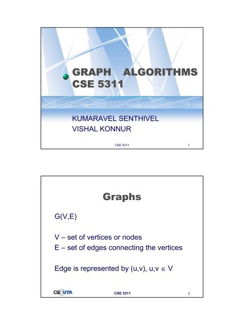
G(V,E)<br />
<strong>GRAPH</strong> <strong>ALGORITHMS</strong><br />
<strong>CSE</strong> <strong>5311</strong><br />
KUMARAVEL SENTHIVEL<br />
VISHAL KONNUR<br />
<strong>CSE</strong> <strong>5311</strong> 1<br />
<strong>Graphs</strong><br />
V – set of vertices or nodes<br />
E – set of edges connecting the vertices<br />
Edge is represented by (u,v), u,v ∈ V<br />
<strong>CSE</strong> <strong>5311</strong> 2
Directed & Undirected<br />
1 2<br />
5 4<br />
3<br />
1 2<br />
5 4<br />
Undirected Graph Directed Graph<br />
Degree Number of edges connected to the vertex<br />
In-degree Number of edges coming in to the vertex<br />
Out-degree Number of edges going out of the vertex<br />
<strong>CSE</strong> <strong>5311</strong> 3<br />
Graph Representation<br />
Adjacency Lists<br />
Preferred for Sparse <strong>Graphs</strong> E |V| 2<br />
Requires Θ(|V| 2 ) memory spaces<br />
To determine connectivity between vertices<br />
Used by all-pairs shortest-paths algorithms<br />
<strong>CSE</strong> <strong>5311</strong> 4<br />
3
1 2<br />
5 4<br />
1 2<br />
5 4<br />
Adjacency List<br />
3<br />
1 2 5 /<br />
2<br />
3<br />
4<br />
5<br />
1<br />
2<br />
2<br />
4<br />
5 3<br />
4 /<br />
5<br />
1<br />
3 /<br />
2 /<br />
<strong>CSE</strong> <strong>5311</strong> 5<br />
Adjacency Matrix<br />
3<br />
1<br />
2<br />
3<br />
4<br />
5<br />
1<br />
0<br />
1<br />
0<br />
0<br />
1<br />
2<br />
1<br />
0<br />
1<br />
1<br />
1<br />
<strong>CSE</strong> <strong>5311</strong> 6<br />
3<br />
0<br />
1<br />
0<br />
1<br />
0<br />
4<br />
0<br />
1<br />
1<br />
0<br />
1<br />
4 /<br />
5<br />
1<br />
1<br />
0<br />
1<br />
0
Graph Terminology<br />
Path: A path between two nodes is a<br />
sequence of intermediate nodes connected<br />
by edges<br />
Cycle: A path in a graph is a cycle if its first<br />
and last vertices are identical, no other vertex<br />
appears more than once and if it contains at<br />
least two distinct edges<br />
Loop: A loop is an edge with the start and the<br />
end nodes are the same<br />
<strong>CSE</strong> <strong>5311</strong> 7<br />
Graph Terminology<br />
Connected Graph: A graph in which all nodes are<br />
connected<br />
Forest: A graph that has more than one connected<br />
component<br />
Acyclic Graph: A graph that doesn’t contain any<br />
cycle<br />
Tree: Connected Acyclic graph is called a tree<br />
Spanning Tree: A sub tree of a graph having all the<br />
nodes of the graph<br />
<strong>CSE</strong> <strong>5311</strong> 8
Breadth First Search<br />
Simple algorithm to search a graph<br />
Works on both directed and undirected<br />
graphs<br />
Given a source, S ∈ V, it discovers<br />
every other reachable vertex.<br />
It produces the breadth-first tree with<br />
shortest paths between S and other<br />
vertices<br />
<strong>CSE</strong> <strong>5311</strong> 9<br />
BFS<br />
Breadth First Search, starts at any node<br />
(Level 0) of the graph and then scans<br />
for the nearest neighbors at Level 1.<br />
Then it scans for the nodes at Level 2<br />
for all nodes at Level 1<br />
The algorithm ends when all nodes are<br />
visited<br />
Uses Queue to store the visited nodes<br />
<strong>CSE</strong> <strong>5311</strong> 10
BFS(G(V,E),s)<br />
BFS: pseudo-code<br />
for each vertex u ∈ V[G] – {s}<br />
color[u] = white<br />
dist[u] = ∞<br />
end for<br />
color[s] = gray<br />
dist[s] = 0<br />
T=null<br />
Q=null<br />
Add(Q, s)<br />
while Q ≠ null<br />
u = Delete(Q, s)<br />
for each v ∈ Adj_List[u]<br />
if color[v] = white<br />
color[v] = gray<br />
dist[v] = dist[u] + 1<br />
T = T U (u,v)<br />
Add(Q, v)<br />
end if<br />
end for<br />
color[u] = black<br />
end while<br />
<strong>CSE</strong> <strong>5311</strong> 11<br />
BFS: Example<br />
r s t u<br />
∞ 1 0 ∞ 2<br />
∞ 3<br />
∞2 ∞ 1<br />
Q<br />
T<br />
s<br />
∞ 2<br />
∞3<br />
v w x y<br />
w r<br />
t x v u y<br />
s,w s,r w,t w,x r,v t,u x,y<br />
<strong>CSE</strong> <strong>5311</strong> 12
BFS: Run Time Analysis<br />
Initialization takes O(|V|) time<br />
Adding and Deleting an element in Queue<br />
takes O(1) time. Total time for queue<br />
operations is O(|V|)<br />
In the iteration the adjacency list of every<br />
vertex is scanned at most once. Sum of all<br />
lengths of all adjacency lists is Θ(|E|). Total<br />
time for scanning the list is O(|E|)<br />
Total Running Time of BFS is O(|V| + |E|)<br />
<strong>CSE</strong> <strong>5311</strong> 13<br />
BFS: Applications<br />
Compute Connected Components of a<br />
graph<br />
Compute a spanning tree of a graph<br />
Find a cycle in a graph<br />
Find whether the graph is a forest<br />
A path between two vertices with<br />
minimum number of edges<br />
<strong>CSE</strong> <strong>5311</strong> 14
Depth First Search<br />
DFS scans for the neighbors at Level 1.<br />
When it finds the first neighbor, the algorithm<br />
proceeds to scan its neighbors at Level 2.<br />
Goes as deep into the graph as possible<br />
The algorithm is recursive and ends when all<br />
the nodes are visited<br />
Uses Stack implicitly<br />
<strong>CSE</strong> <strong>5311</strong> 15<br />
DFS: pseudo-code<br />
DFS(G(V,E))<br />
for each vertex u ∈ V[G]<br />
color[u] = white<br />
p[u] = nil<br />
end for<br />
time = 0<br />
for each vertex u ∈ V[G]<br />
if color[u] = white<br />
DFS-Visit(u)<br />
end if<br />
end for<br />
DFS-Visit(u)<br />
color[u] = gray<br />
time = time + 1<br />
d[u] = time<br />
for each v ∈ Adj[u]<br />
if color[v] = white<br />
p[v] = u<br />
DFS-Visit(v)<br />
end if<br />
end for<br />
color[u] = black<br />
f[u] = time = time + 1<br />
<strong>CSE</strong> <strong>5311</strong> 16
7<br />
4<br />
5<br />
DFS: Example<br />
3<br />
6<br />
8<br />
2<br />
1<br />
13<br />
11<br />
9<br />
10<br />
12<br />
<strong>CSE</strong> <strong>5311</strong> 17<br />
DFS: Run Time Analysis<br />
The two loops in DFS procedure takes O(|V|)<br />
time, exclusive of time to call DFS-Visit<br />
DFS-Visit is called only once for each vertex<br />
DFS-Visit scans the Adjacency list. Sum of all<br />
lengths of all adjacency lists is Θ(|E|). Total<br />
time for scanning the list is O(|E|)<br />
Total Running Time of DFS is O(|V| + |E|)<br />
<strong>CSE</strong> <strong>5311</strong> 18
DFS: Applications<br />
Connected Components<br />
Topological Sort<br />
Find a cycle in a graph<br />
Find whether the graph is a forest<br />
<strong>CSE</strong> <strong>5311</strong> 19<br />
DFS vs. BFS<br />
When a breadth-first search succeeds, it finds a<br />
minimum-depth (nearest the root) goal node<br />
When a depth-first search succeeds, the found goal<br />
node is not necessarily minimum depth<br />
For a large tree, a depth-first search may take an<br />
excessively long time to find even a very nearby goal<br />
node, where as breadth-first search can find the<br />
nearby nodes faster.<br />
<strong>CSE</strong> <strong>5311</strong> 20
Connected Components<br />
Problem: Two vertices are in the same<br />
component of G if and only if there is<br />
some path between them. Find the<br />
number of components in a graph<br />
Input : A directed or undirected graph<br />
G. A start vertex s<br />
<strong>CSE</strong> <strong>5311</strong> 21<br />
Connected Components<br />
pseudo-code<br />
Procedure Connected_Components G(V,E)<br />
Input : G (V,E)<br />
Output : Number of Connected Components<br />
V' ← V;<br />
c ← 0;<br />
while V' ≠ 0 do<br />
choose u ∈ V' ;<br />
T ← all nodes reachable from u (by DFS_Tree)<br />
V' ←V' - T;<br />
c ← c+1;<br />
G c ← T;<br />
T ← 0;<br />
<strong>CSE</strong> <strong>5311</strong> 22
Connected Components<br />
Example<br />
Input Output<br />
<strong>CSE</strong> <strong>5311</strong> 23<br />
Topological Sort<br />
Problem: Find a linear ordering of the<br />
vertices of V such that for each edge<br />
(i,j) in E, vertex i is to the left of vertex j.<br />
Input : A directed, acyclic graph<br />
G=(V,E)<br />
<strong>CSE</strong> <strong>5311</strong> 24
Topological Sort<br />
pseudo-code<br />
TopologicalSort(G)<br />
1. DFS(G)<br />
2. As each vertex finishes, insert it on<br />
the front of a linked list<br />
3. Return linked list of vertices<br />
<strong>CSE</strong> <strong>5311</strong> 25<br />
Topological Sort<br />
Example<br />
Input Output<br />
6<br />
10<br />
5<br />
8<br />
4<br />
<strong>CSE</strong> <strong>5311</strong> 26<br />
2<br />
9<br />
3<br />
1<br />
7
Minimum Cost Spanning Tree<br />
Find a tree formed from graph edges<br />
that connects all the vertices in G, at<br />
minimum cost<br />
Kruskal’s Algorithm<br />
Prim’s Algorithm<br />
<strong>CSE</strong> <strong>5311</strong> 27<br />
Kruskal’s algorithm<br />
It is a greedy algorithm which sorts<br />
the edges in the order of minimum<br />
weight and adds them to the tree, till<br />
all the nodes are added<br />
The set formed is a forest and the<br />
edges that connects the forests are<br />
also included<br />
<strong>CSE</strong> <strong>5311</strong> 28
Kruskal’s algorithm<br />
pseudo-code<br />
Algorithm KruskalMST(G)<br />
T ← 0;<br />
VS ←0;<br />
for each vertex v ∈ V do<br />
VS = VS ∪ {v};<br />
sort the edges of E in non-decreasing order of weight<br />
while |VS| > 1 do<br />
choose (v,w) an edge E of lowest cost;<br />
delete (v,w) from E;<br />
if v and w are in different sets W1 and W2 in VS do<br />
W1 = W1 ∪ W2;<br />
VS = VS - W2;<br />
T ← T∪ (v,w);<br />
return T<br />
<strong>CSE</strong> <strong>5311</strong> 29<br />
Kruskal’s Algorithm<br />
Example<br />
8<br />
B<br />
C<br />
6<br />
6<br />
6<br />
E<br />
2<br />
1<br />
7<br />
A<br />
D<br />
2<br />
E D C B A<br />
<strong>CSE</strong> <strong>5311</strong> 30
Kruskal’s Algorithm<br />
Example<br />
8<br />
B<br />
C<br />
6<br />
6<br />
6<br />
E<br />
2<br />
1<br />
7<br />
A<br />
D<br />
2<br />
E D C B A<br />
<strong>CSE</strong> <strong>5311</strong> 31<br />
Kruskal’s Algorithm<br />
Example<br />
8<br />
B<br />
C<br />
6<br />
6<br />
6<br />
E<br />
2<br />
1<br />
7<br />
A<br />
D<br />
2<br />
E D C B A<br />
<strong>CSE</strong> <strong>5311</strong> 32
Kruskal’s Algorithm<br />
Example<br />
8<br />
B<br />
C<br />
6<br />
6<br />
6<br />
E<br />
2<br />
1<br />
7<br />
A<br />
D<br />
2<br />
E D C B A<br />
<strong>CSE</strong> <strong>5311</strong> 33<br />
Kruskal’s Algorithm<br />
Example<br />
8<br />
B<br />
C<br />
6<br />
6<br />
6<br />
E<br />
2<br />
1<br />
7<br />
A<br />
D<br />
2<br />
E D C B A<br />
<strong>CSE</strong> <strong>5311</strong> 34
Kruskal’s Algorithm<br />
Run Time Analysis<br />
Sorting the edges take O(E log E) time<br />
Adding the edges to the tree takes O(E)<br />
time<br />
So, the running time for the algorithm is<br />
in O(E log E)<br />
<strong>CSE</strong> <strong>5311</strong> 35<br />
Prim’s Algorithm<br />
Prim’s algorithm for minimum spanning<br />
trees has a similar style to Dijkstra’s<br />
algorithm for shortest paths<br />
The set formed is always a tree<br />
The edge with minimum weight added<br />
always connects a node that is not in<br />
the tree<br />
<strong>CSE</strong> <strong>5311</strong> 36
Prim’s algorithm<br />
pseudo-code<br />
Algorithm PrimMST(G, r)<br />
for each vertex v ∈ V do<br />
key[u] = infinity<br />
T= NIL<br />
key[r] = 0<br />
Q = V<br />
T = NULL<br />
while Q ≠ NULL do<br />
u = Extract-Min(Q)<br />
for each v ∈ Adj[u]<br />
if v ∈ Q and w(u,v) < key[v]<br />
key[v] = w(u,v)<br />
T ← T∪ (u,v)<br />
return T<br />
<strong>CSE</strong> <strong>5311</strong> 37<br />
Prim’s Algorithm<br />
Example<br />
4<br />
v1<br />
2<br />
v2<br />
2<br />
7<br />
v3 v4 v5<br />
5<br />
8<br />
1 3<br />
v6 v7<br />
1<br />
The minimum spanning tree is shown with bold edges.<br />
The total edge cost is 16.<br />
4<br />
10<br />
<strong>CSE</strong> <strong>5311</strong> 38<br />
6
Prim’s Algorithm<br />
Example<br />
4<br />
v1<br />
2<br />
v2<br />
2<br />
7<br />
v3 v4 v5<br />
5<br />
8<br />
1 3<br />
v6 v7<br />
1<br />
We start with v1, and place this into the tree. The rest of<br />
the vertices are not in the tree. The cheapest edge we can<br />
add from v1 to the other vertices is (v1, v4).<br />
v1<br />
4<br />
10<br />
<strong>CSE</strong> <strong>5311</strong> 39<br />
Prim’s Algorithm<br />
Example<br />
4<br />
2<br />
v2<br />
2<br />
7<br />
v3 v4 v5<br />
5<br />
8<br />
1 3<br />
v6 v7<br />
1<br />
Now v1 and v4 are in the tree. The cheapest edge we can add<br />
is either (v1, v2) or (v4, v3). We choose (v1, v2).<br />
4<br />
<strong>CSE</strong> <strong>5311</strong> 40<br />
6<br />
10<br />
6
Prim’s Algorithm<br />
Example<br />
4<br />
v1<br />
2<br />
v2<br />
2<br />
7<br />
v3 v4 v5<br />
5<br />
8<br />
1 3<br />
v6 v7<br />
1<br />
Now v1, v2, and v4 are in the tree. The cheapest edge we<br />
can add is (v4, v3).<br />
v1<br />
4<br />
10<br />
<strong>CSE</strong> <strong>5311</strong> 41<br />
Prim’s Algorithm<br />
Example<br />
4<br />
2<br />
v2<br />
2<br />
7<br />
v3 v4 v5<br />
5<br />
8<br />
1 3<br />
v6 v7<br />
1<br />
Now v1, v2, v3, and v4 are in the tree. The cheapest edge we<br />
can add is (v4, v7).<br />
4<br />
<strong>CSE</strong> <strong>5311</strong> 42<br />
6<br />
10<br />
6
Prim’s Algorithm<br />
Example<br />
4<br />
v1<br />
2<br />
v2<br />
2<br />
7<br />
v3 v4 v5<br />
5<br />
8<br />
1 3<br />
v6 v7<br />
1<br />
Now v1, v2, v3, v4, and v7 are in the tree. The cheapest edge we<br />
can add is (v7, v6).<br />
v1<br />
4<br />
10<br />
<strong>CSE</strong> <strong>5311</strong> 43<br />
Prim’s Algorithm<br />
Example<br />
4<br />
2<br />
v2<br />
2<br />
7<br />
v3 v4 v5<br />
5<br />
8<br />
1 3<br />
v6 v7<br />
1<br />
Now v1, v2, v3, v4, v6 and v7 are in the tree. The cheapest edge<br />
we can add is (v7, v5). We are now done. This is optimal.<br />
4<br />
<strong>CSE</strong> <strong>5311</strong> 44<br />
6<br />
10<br />
6
Prim’s Algorithm<br />
Run Time analysis<br />
The initialization takes O(V) time<br />
The Extract-Min takes O(log V) time if it is<br />
implemented as binary heap<br />
For V iterations Extract-Min takes O(VlogV)<br />
time<br />
The key assignment takes O(log V) time<br />
For all edges the key assignment takes O(E<br />
log V) time.<br />
Hence the total time is O(VlogV + ElogV) =<br />
O(ElogV). This is same as Kruskal’s algorithm<br />
<strong>CSE</strong> <strong>5311</strong> 45<br />
MCST: Applications<br />
Used in Networking protocols<br />
Multicast Routing<br />
<strong>CSE</strong> <strong>5311</strong> 46
Single Source Shortest<br />
Path<br />
Given graph (directed or undirected) G =<br />
(V,E) with weight function w: E → R and a<br />
vertex s, find for all vertices in V the minimum<br />
possible weight for path from s to v.<br />
BellMan-Ford’s Algorithm<br />
Dijkstra’s Algorithm<br />
<strong>CSE</strong> <strong>5311</strong> 47<br />
Relaxing an Edge<br />
Relaxing an edge consists of testing whether<br />
we can improve the shortest path to v by<br />
going through u<br />
If there is a shortest path then update<br />
Distance[v] and Predecessor[v]=u<br />
Relax(u,v)<br />
If d[v] > d[u] + w(u,v)<br />
d[v] = d[u] + w(u,v)<br />
p[v] = u<br />
<strong>CSE</strong> <strong>5311</strong> 48
Bellman-Ford’s<br />
Algorithm<br />
The algorithm uses relaxation<br />
The d[v], the weight of the path from<br />
source s to destination v, is relaxed<br />
progressively until it reaches the<br />
minimum weight<br />
The algorithm returns true only if the<br />
graph does not contain any negative<br />
cycles<br />
<strong>CSE</strong> <strong>5311</strong> 49<br />
Bellman-Ford’s<br />
Algorithm pseudo-code<br />
BellmanFord(graph (G,w), vertex s)<br />
for each vertex v ∈ V<br />
d[v] = infinity<br />
p[v] = NIL<br />
d[s] = 0<br />
for i ← 1 to |V| - 1 do<br />
for (u,v) ∈ E[G] do<br />
Relax(u,v)<br />
for (u,v) ∈ E[G] do<br />
if d[v] > d[u] + w(u,v) then<br />
return false<br />
return true<br />
<strong>CSE</strong> <strong>5311</strong> 50
Bellman-Ford’s<br />
Algorithm Example<br />
6<br />
7<br />
8<br />
-2<br />
9<br />
-3<br />
2<br />
5<br />
-4<br />
7<br />
<strong>CSE</strong> <strong>5311</strong> 51<br />
Bellman-Ford’s<br />
Algorithm Example<br />
0<br />
6<br />
7<br />
∞<br />
∞<br />
8<br />
-2<br />
9<br />
-3<br />
2<br />
5<br />
-4<br />
∞<br />
∞<br />
7<br />
<strong>CSE</strong> <strong>5311</strong> 52
Bellman-Ford’s<br />
Algorithm Example<br />
0<br />
6<br />
7<br />
6<br />
7<br />
8<br />
-2<br />
9<br />
-3<br />
2<br />
5<br />
-4<br />
∞<br />
∞<br />
7<br />
<strong>CSE</strong> <strong>5311</strong> 53<br />
Bellman-Ford’s<br />
Algorithm Example<br />
0<br />
6<br />
7<br />
6<br />
7<br />
8<br />
-2<br />
9<br />
-3<br />
2<br />
5<br />
-4<br />
4<br />
2<br />
7<br />
<strong>CSE</strong> <strong>5311</strong> 54
Bellman-Ford’s<br />
Algorithm Example<br />
0<br />
6<br />
7<br />
2<br />
7<br />
8<br />
-2<br />
9<br />
-3<br />
2<br />
5<br />
-4<br />
4<br />
2<br />
7<br />
<strong>CSE</strong> <strong>5311</strong> 55<br />
Bellman-Ford’s<br />
Algorithm Example<br />
0<br />
6<br />
7<br />
2<br />
7<br />
8<br />
-2<br />
9<br />
-3<br />
2<br />
5<br />
-4<br />
4<br />
-2<br />
7<br />
<strong>CSE</strong> <strong>5311</strong> 56
Bellman-Ford’s Algorithm<br />
Run Time Analysis<br />
The Bellman-Ford algorithm computes<br />
the distance from source s to all other<br />
vertices of G<br />
Determine that G contains a negativeweight<br />
cycle,<br />
In O(VE) time<br />
<strong>CSE</strong> <strong>5311</strong> 57<br />
Dijkstra’s Algorithm<br />
Faster than Bellman-Ford’s Algorithm<br />
Dijkstra’s algorithm is based on the<br />
greedy method<br />
It starts with the source and builds the<br />
spanning tree by adding one edge at a<br />
time which gives the shortest path from<br />
the source to the vertex not in the<br />
spanning tree<br />
<strong>CSE</strong> <strong>5311</strong> 58
Dijkstras Algorithm<br />
pseudo-code<br />
Dijkstra(G,s)<br />
for each vertex v ∈ V<br />
d[v] = infinity<br />
p[v] = NIL<br />
d[s] = 0<br />
S = NULL<br />
Q = V<br />
while Q ≠ NULL do<br />
u = Extract-Min(Q)<br />
S ← S∪ {u}<br />
for each v ∈ Adj[u]<br />
Relax(u,v)<br />
<strong>CSE</strong> <strong>5311</strong> 59<br />
Dijkistra’s Algorithm<br />
It assumes the path length does not increase when more edges<br />
are added to the path. If a node with a negative incident edge<br />
were to be added late to the vertex list for which decisions have<br />
been made, it could mess up distances for vertices already in<br />
the list.<br />
This is almost identical to that of Prim's algorithm. The only<br />
difference here is that the Dijkstra's algorithm stores the<br />
distance from the source to current vertex, while Prim's<br />
algorithm stores the cost of the minimum-cost edge connecting<br />
a vertex in V to u.<br />
<strong>CSE</strong> <strong>5311</strong> 60
e<br />
Dijkstra’s Algorithm<br />
Example<br />
2<br />
4<br />
4<br />
d<br />
1<br />
f<br />
1<br />
b<br />
1<br />
4<br />
4<br />
1<br />
c<br />
4<br />
a<br />
D [ a b c d e f ] C<br />
x x x 0 x x φ<br />
x x 4 0 2 x {d}<br />
x 6 3 0 2 6 {d,e}<br />
7 4 3 0 2 6 {c,d,e}<br />
7 4 3 0 2 5 {b,c,d,e}<br />
6 4 3 0 2 5 {b,c,d,e,f}<br />
6 4 3 0 2 5 {a,b,c,d,e,f}<br />
<strong>CSE</strong> <strong>5311</strong> 61<br />
Dijkstra’s Algorithm<br />
Example<br />
10<br />
5<br />
2 3<br />
2<br />
9<br />
1<br />
7<br />
4<br />
<strong>CSE</strong> <strong>5311</strong> 62<br />
6
Dijkstra’s Algorithm<br />
Example<br />
0<br />
10<br />
5<br />
∞<br />
2 3<br />
∞<br />
2<br />
9<br />
1<br />
7<br />
4<br />
∞<br />
∞<br />
<strong>CSE</strong> <strong>5311</strong> 63<br />
Dijkstra’s Algorithm<br />
Example<br />
0<br />
10<br />
5<br />
10<br />
2 3<br />
5<br />
2<br />
9<br />
1<br />
7<br />
4<br />
∞<br />
∞<br />
<strong>CSE</strong> <strong>5311</strong> 64<br />
6<br />
6
Dijkstra’s Algorithm<br />
Example<br />
0<br />
10<br />
5<br />
10<br />
2 3<br />
5<br />
2<br />
9<br />
1<br />
7<br />
4<br />
∞<br />
∞<br />
<strong>CSE</strong> <strong>5311</strong> 65<br />
Dijkstra’s Algorithm<br />
Example<br />
0<br />
10<br />
5<br />
8<br />
2 3<br />
5<br />
2<br />
9<br />
1<br />
7<br />
4<br />
14<br />
7<br />
<strong>CSE</strong> <strong>5311</strong> 66<br />
6<br />
6
Dijkstra’s Algorithm<br />
Example<br />
0<br />
10<br />
5<br />
8<br />
2 3<br />
5<br />
2<br />
9<br />
1<br />
7<br />
4<br />
14<br />
7<br />
<strong>CSE</strong> <strong>5311</strong> 67<br />
Dijkstra’s Algorithm<br />
Example<br />
0<br />
10<br />
5<br />
8<br />
2 3<br />
5<br />
2<br />
9<br />
1<br />
7<br />
4<br />
13<br />
7<br />
<strong>CSE</strong> <strong>5311</strong> 68<br />
6<br />
6
Dijkstra’s Algorithm<br />
Example<br />
0<br />
10<br />
5<br />
8<br />
2 3<br />
5<br />
2<br />
9<br />
1<br />
7<br />
4<br />
13<br />
7<br />
<strong>CSE</strong> <strong>5311</strong> 69<br />
Dijkstra’s Algorithm<br />
Example<br />
0<br />
10<br />
5<br />
8<br />
2 3<br />
5<br />
2<br />
9<br />
1<br />
7<br />
4<br />
9<br />
7<br />
<strong>CSE</strong> <strong>5311</strong> 70<br />
6<br />
6
Dijkstra’s Algorithm<br />
Example<br />
0<br />
10<br />
5<br />
8<br />
2 3<br />
5<br />
2<br />
9<br />
1<br />
7<br />
4<br />
9<br />
7<br />
<strong>CSE</strong> <strong>5311</strong> 71<br />
Dijkstra’s Algorithm<br />
Run Time Analysis<br />
The initialisation takes O(V) time<br />
There are V iterations of Extract-Min<br />
There are E iterations of distance assignment<br />
Time = V x TimeExtract-Min + E x Timedist assign<br />
Array<br />
Q<br />
Binary Heap<br />
Fibonacci<br />
Heap<br />
T EXTARCT-MIN<br />
O(V)<br />
O(log V)<br />
O(log V)<br />
T DIST-ASSIGN<br />
1<br />
O(log V)<br />
1<br />
<strong>CSE</strong> <strong>5311</strong> 72<br />
6<br />
Total Time<br />
O(V<br />
O(E logV)<br />
O(E + V log V)<br />
2 )
SSSP: Applications<br />
Used in Routing Protocols<br />
Dijkstra’s Algorithm is used in Link State<br />
Routing<br />
Bellman-Ford’s Algorithm is used in<br />
Distance Vector Routing<br />
<strong>CSE</strong> <strong>5311</strong> 73<br />
All Pairs Shortest Path<br />
The all-pairs-shortest-path problem is<br />
generalization of the single-sourceshortest-path<br />
problem for all nodes.<br />
Problem is to find the shortest paths<br />
between all pairs of vertices Vi ,Vj ∈ V<br />
such that i ≠ j.<br />
<strong>CSE</strong> <strong>5311</strong> 74
Floyd’s Algorithm<br />
d s,t (i) – the shortest path from s to t<br />
containing only vertices v 1 , ..., v i<br />
d s,t (0) = w(s,t)<br />
d (k)<br />
s,t = w(s,t) if k = 0<br />
min{d (k-1)<br />
s,t , ds,k<br />
(k-1) + dk,t<br />
(k-1) }<br />
if k > 0<br />
<strong>CSE</strong> <strong>5311</strong> 75<br />
Floyd’s Algorithm<br />
pseudo-code<br />
FloydWarshall (matrix W, integer n)<br />
D (0) ← W<br />
for k ← 1 to n do<br />
for i ← 1 to n do<br />
for j ← 1 to n do<br />
d (k)<br />
ij ← min(dij (k-1) , dik<br />
(k-1) + dkj<br />
(k-1) )<br />
return D (n)<br />
<strong>CSE</strong> <strong>5311</strong> 76
3<br />
Floyd’s Algorithm<br />
Example<br />
2<br />
7 1<br />
1 3<br />
-4<br />
8<br />
2<br />
5 4<br />
6<br />
2<br />
4<br />
-5<br />
1 3<br />
8<br />
-4<br />
3<br />
7<br />
1<br />
2<br />
3<br />
4<br />
5<br />
1<br />
0<br />
∞<br />
∞<br />
2<br />
∞<br />
Adjacency Matrix<br />
2<br />
3<br />
0<br />
4<br />
∞<br />
∞<br />
∞<br />
-5<br />
∞<br />
∞<br />
<strong>CSE</strong> <strong>5311</strong> 77<br />
Floyd’s Algorithm<br />
Example<br />
2<br />
1<br />
5 4<br />
6<br />
4<br />
-5<br />
1<br />
2<br />
3<br />
4<br />
5<br />
3<br />
8<br />
0<br />
4<br />
∞<br />
1<br />
0<br />
6<br />
Shortest Path Matrix D (1)<br />
1<br />
0<br />
∞<br />
∞<br />
2<br />
∞<br />
2<br />
3<br />
0<br />
4<br />
∞<br />
∞<br />
5<br />
-4<br />
7<br />
∞<br />
∞<br />
<strong>CSE</strong> <strong>5311</strong> 78<br />
3<br />
8<br />
0<br />
4<br />
∞<br />
1<br />
0<br />
5<br />
-4<br />
7<br />
∞<br />
∞5<br />
-5 0 -2 ∞<br />
∞ ∞ 6 0
3<br />
7<br />
2<br />
1 3<br />
8<br />
-4<br />
Floyd’s Algorithm<br />
Example<br />
2<br />
1<br />
5 4<br />
6<br />
4<br />
-5<br />
3<br />
2<br />
4<br />
7<br />
1<br />
1 3<br />
8<br />
-4<br />
1<br />
2<br />
3<br />
4<br />
5<br />
Shortest Path Matrix D (2)<br />
1<br />
0<br />
∞<br />
∞<br />
2<br />
∞<br />
2<br />
3<br />
0<br />
4<br />
5<br />
∞<br />
∞<br />
-5<br />
∞<br />
∞5<br />
11 ∞<br />
<strong>CSE</strong> <strong>5311</strong> 79<br />
Floyd’s Algorithm<br />
Example<br />
2<br />
5 4<br />
6<br />
-5<br />
1<br />
2<br />
3<br />
4<br />
5<br />
3<br />
8<br />
0<br />
4<br />
4<br />
1<br />
0<br />
6<br />
Shortest Path Matrix D (3)<br />
1<br />
0<br />
∞<br />
∞<br />
2<br />
∞<br />
2<br />
3<br />
0<br />
4<br />
-1 5<br />
∞<br />
∞<br />
-5<br />
∞<br />
5<br />
-4<br />
7<br />
-2<br />
<strong>CSE</strong> <strong>5311</strong> 80<br />
3<br />
8<br />
0<br />
4<br />
4<br />
1<br />
5<br />
0<br />
6<br />
0<br />
5<br />
-4<br />
7<br />
11<br />
-2<br />
0
3<br />
7<br />
2<br />
1 3<br />
8<br />
-4<br />
Floyd’s Algorithm<br />
Example<br />
2<br />
1<br />
5 4<br />
6<br />
4<br />
-5<br />
3<br />
2<br />
4<br />
7<br />
1<br />
1 3<br />
8<br />
-4<br />
1<br />
2<br />
3<br />
4<br />
5<br />
Shortest Path Matrix D (4)<br />
1<br />
0<br />
∞3<br />
0 -4 ∞ 1 -1 7<br />
∞7<br />
2<br />
2<br />
3<br />
4<br />
-1<br />
-1 8<br />
-5<br />
∞8<br />
∞5<br />
∞1<br />
<strong>CSE</strong> <strong>5311</strong> 81<br />
Floyd’s Algorithm<br />
Example<br />
2<br />
5 4<br />
6<br />
-5<br />
1<br />
2<br />
3<br />
4<br />
5<br />
3<br />
0<br />
4<br />
4<br />
5<br />
0<br />
6<br />
Shortest Path Matrix D (5)<br />
1<br />
0<br />
3<br />
7<br />
2<br />
8<br />
2<br />
3<br />
0<br />
4<br />
-1<br />
5<br />
-5<br />
5<br />
-4<br />
11 3<br />
-2<br />
<strong>CSE</strong> <strong>5311</strong> 82<br />
3<br />
-1<br />
-4<br />
0<br />
1<br />
4<br />
24<br />
1<br />
5<br />
0<br />
6<br />
0<br />
5<br />
-4<br />
-1<br />
3<br />
-2<br />
0
3<br />
7<br />
2<br />
1 3<br />
8<br />
-4<br />
Floyd’s Algorithm<br />
Example<br />
2<br />
1<br />
5 4<br />
6<br />
4<br />
-5<br />
1<br />
2<br />
3<br />
4<br />
5<br />
Shortest Path Matrix D (5)<br />
3<br />
7<br />
2<br />
8<br />
0<br />
4<br />
-1<br />
5<br />
-1<br />
-4<br />
-5<br />
<strong>CSE</strong> <strong>5311</strong> 83<br />
Floyd’s Algorithm<br />
Run Time Analysis<br />
Running Time of O(|V| 3 )<br />
Negatively weighed edges may be<br />
present.<br />
Negatively weighted cycles cause<br />
problems with the algorithm.<br />
1<br />
0<br />
2<br />
3<br />
3<br />
0<br />
1<br />
4<br />
2<br />
1<br />
5<br />
0<br />
6<br />
5<br />
-4<br />
-1<br />
3<br />
-2<br />
<strong>CSE</strong> <strong>5311</strong> 84<br />
0
Negative Cycle<br />
Detection<br />
Execute Floyd’s Algorithm. If at least<br />
one diagonal entry contain a negative<br />
value then there is a negative cycle<br />
Complexity is O(V 3 )<br />
Execute Bellman-Ford Algorithm. If it<br />
returns false then the graph contain a<br />
negative cycle<br />
Complexity is O(VE)<br />
<strong>CSE</strong> <strong>5311</strong> 85<br />
Faster Algorithm for All<br />
Source Shortest Path<br />
Try using the existing Single Source<br />
Shortest Path for all sources<br />
If Bellman-Ford’s algorithm is again to<br />
find the shortest paths for all sources<br />
then the complexity is O(V2E) = O(V4 )<br />
Bellman-Ford’s algorithm is worse than<br />
Floyd’s algorithm<br />
<strong>CSE</strong> <strong>5311</strong> 86
Faster Algorithm for<br />
All Source Shortest Path<br />
Use Dijkstra’s Algorithm to compute<br />
shortest paths for all sources<br />
Runs in time O(V (E log V)) with binary<br />
heap and O(V*(E + V log V) with<br />
Fibonacci heaps<br />
But cannot have negative edges<br />
<strong>CSE</strong> <strong>5311</strong> 87<br />
Reweighting the edges<br />
A reweighting function ŵ should satisfy<br />
two properties<br />
For all pairs of vertices u, u ∈ V, a path p is<br />
a shortest path from u to v using the weight<br />
function w if and only if p is also a shortest<br />
path from u to v using weight function ŵ<br />
For all edges (u,v) the new weight ŵ(u,v) is<br />
non-negative<br />
<strong>CSE</strong> <strong>5311</strong> 88
Reweighting the edges<br />
For a weighted, directed graph G=(V,E)<br />
with weight function<br />
w : E → R (weight of edges)<br />
h : V → R (distance vector calculated using<br />
Bellman-Ford’s algorithm)<br />
ŵ(u,v) = w(u,v) + ( h(u) – h(v) )<br />
<strong>CSE</strong> <strong>5311</strong> 89<br />
Johnson’s Algorithm<br />
1. Add a node S to the graph with zero<br />
weight edges connecting to all nodes<br />
of the graph<br />
It is done to calculate the weighting<br />
function using Bellman-Ford’s algorithm.<br />
If any one node does not have path to all<br />
other nodes then the weight of some<br />
nodes will be infinite<br />
<strong>CSE</strong> <strong>5311</strong> 90
Johnson’s Algorithm<br />
2. Execute Bellman-Ford’s algorithm on<br />
the new graph<br />
3. If it returns false then there is a<br />
negative cycle in the graph and hence<br />
abort the algorithm<br />
4. Reweigh all the edges<br />
<strong>CSE</strong> <strong>5311</strong> 91<br />
Johnson’s algorithm<br />
5. For all nodes execute Dijkstra’s<br />
algorithm to find the shortest path to<br />
all other nodes<br />
6. Recalculate the correct shortest-path<br />
weight<br />
dist(u)(v) = ĝ(u,v) – (h(v) – h(u))<br />
<strong>CSE</strong> <strong>5311</strong> 92
Johnson’s algorithm<br />
Example<br />
-4<br />
3<br />
7<br />
6<br />
2<br />
8<br />
1<br />
Original Graph<br />
4<br />
-5<br />
<strong>CSE</strong> <strong>5311</strong> 93<br />
Johnson’s algorithm<br />
Example<br />
0<br />
s<br />
0<br />
0<br />
0<br />
-4<br />
0<br />
3<br />
7<br />
Graph with the ‘s’ node added with zero weight edges<br />
6<br />
2<br />
0<br />
8<br />
1<br />
4<br />
-5<br />
<strong>CSE</strong> <strong>5311</strong> 94
Johnson’s algorithm<br />
Example<br />
0<br />
s<br />
0<br />
0<br />
0<br />
0<br />
-4<br />
0<br />
3<br />
-4<br />
7<br />
Weight function calculated using Bellman Ford’s algorithm<br />
-1<br />
6<br />
2<br />
0<br />
8<br />
1<br />
0<br />
4<br />
-5<br />
-5<br />
<strong>CSE</strong> <strong>5311</strong> 95<br />
Johnson’s algorithm<br />
Example<br />
0<br />
s<br />
0<br />
4<br />
1<br />
0<br />
0<br />
5<br />
4<br />
10<br />
-4<br />
-1<br />
2<br />
2<br />
0<br />
13<br />
0<br />
0<br />
0<br />
-5<br />
-5<br />
Reweighted non-negative edges<br />
<strong>CSE</strong> <strong>5311</strong> 96
x/y<br />
Johnson’s algorithm<br />
Example<br />
0/0<br />
x – weight using Dijkstra’s algorithm<br />
y – actual recalculated weight<br />
0<br />
4<br />
10<br />
0/-4<br />
2/1<br />
2<br />
2<br />
13<br />
0<br />
0<br />
2/2<br />
2/-3<br />
-5<br />
Reweighted non-negative edges<br />
<strong>CSE</strong> <strong>5311</strong> 97<br />
Johnson’s algorithm<br />
Run Time analysis<br />
Find the weighting function h such that w(u, v) >= 0 for<br />
all edges by using Bellman-Ford, or determine that a<br />
negative-weight cycle exists.<br />
• Time = O(VE).<br />
Run Dijkstra’s algorithm from each vertex using w.<br />
• Time = O(VE log V). (when Fibonacci heap is used)<br />
Reweight each shortest-path length w(p) to produce the<br />
shortest-path lengths w(p) of the original graph.<br />
• Time = O(V 2 ).<br />
Total time = O(VE log V). Better for sparse graphs<br />
<strong>CSE</strong> <strong>5311</strong> 98
Representation of<br />
Graph Files<br />
GraphWiz is a set of graph drawing tools<br />
developed by the AT&T Research Labs<br />
Two types of file format<br />
.dot for directed graphs<br />
.neato for undirected graphs<br />
GraphWiz and WinGraphViz are open source<br />
software. Contains both executables and libraries<br />
/* Nodes = 4 */<br />
/* Edges = 5 */<br />
/* Directed = 1 *//**Random**/<br />
/* Min In-Degree = 2 */<br />
/* Max In-Degree = 4 */<br />
/* Min Out-Degree = 2 */<br />
/* Max Out-Degree = 4 */<br />
/* Weighted = 1 */<br />
/* Min Weight = 3 */<br />
/* Max Weight = 10 */<br />
<strong>CSE</strong> <strong>5311</strong> 99<br />
.dot file<br />
digraph G {<br />
size = "7,7";<br />
1 -> 3 [label="6"];<br />
2 -> 3 [label="3"];<br />
2 -> 2 [label="5"];<br />
3 -> 4 [label="7"];<br />
3 -> 3 [label="3"];<br />
}<br />
<strong>CSE</strong> <strong>5311</strong> 100
* Nodes = 4 */<br />
/* Edges = 5 */<br />
/* Directed = 0 *//**Random**/<br />
/* Min Degree = 2 */<br />
/* Max Degree = 4 */<br />
/* Weighted = 1 */<br />
/* Min Weight = 3 */<br />
/* Max Weight = 10 */<br />
.neato file<br />
graph G {<br />
size = "7,7";<br />
1 -- 3 [label="6"];<br />
2 -- 3 [label="3"];<br />
2 -- 2 [label="5"];<br />
3 -- 4 [label="7"];<br />
3 -- 3 [label="3"];<br />
}<br />
<strong>CSE</strong> <strong>5311</strong> 101<br />
<strong>Graphs</strong> Algorithms<br />
Implementation<br />
<strong>CSE</strong> <strong>5311</strong> 102
Graph Algorithms<br />
Implementation<br />
<strong>CSE</strong> <strong>5311</strong> 103<br />
Graph Algorithms<br />
Implementation<br />
<strong>CSE</strong> <strong>5311</strong> 104
References<br />
Thomas H.Cormen, Charles E. Leiserson, Ronald L. Rives,<br />
Clifford Stein, Introduction to Algorithms, 2 nd Edition,<br />
Prentice-Hall<br />
Robert Sedgewick, Algorithms in Java, 3 rd Edition, Addison<br />
Wesley Professional. The sample chapter for Shortest Paths<br />
Graph Algorithms is available at<br />
http://www.informit.com/articles/article.asp?p=169575<br />
Donald B.Johnson, The Pennsylvania state university, Efficient<br />
Algorithms for shortest path in Sparse Networks<br />
WinGraphViz http://www.research.att.com/sw/tools/graphviz<br />
All source shortest paths -<br />
http://compgeom.cs.uiuc.edu/~jeffe/teaching/373/notes/12apsp.pdf<br />
<strong>CSE</strong> <strong>5311</strong> 105