Transport Theory for Light Propagation in Tissues*

Transport Theory for Light Propagation in Tissues*
Arnold D. Kim
Department of Mathematics, Stanford University, USA
ABSTRACT
We review the basic theory for the radiative transport equation governing light propagation in biological tissues.
The Green’s function is the fundamental solution to the transport equation from which all other solutions can
be computed. We compute the Green’s function as an analytical expansion in plane wave modes. We calculate
these plane wave modes numerically using the discrete ordinate method. We use the Green’s function to compute
the point spread function in a half space composed of a uniform scattering and absorbing medium.
1. INTRODUCTION
The radiative transport equation governs light propagation in biological tissue. 1 Hence, solutions of it provide
fundamental insight into the interaction between light and tissue. The Green’s function is the fundamental
solution to the transport equation from which all other solutions can be computed. This theory for the radiative
transport equation is well known. 2, 3 However, the Green’s function is not known except for relatively simple
situations.
We shall describe a method to compute the Green’s function for the transport equation. It is given analytically
as an expansion in plane wave modes. Because plane wave solutions are not known analytically, we calculate
them numerically using a discrete ordinate method. Kim and Keller 4 have given several results regarding plane
wave solutions for the transport equation. In particular, they have identified an important symmetry property.
Kim 5 has extended those results by identifying the orthogonality of plane wave modes. We shall use both the
symmetry and orthogonal properties of plane wave modes to compute the Green’s function.
We shall demonstrate the use of the Green’s function for the transport equation by computing the point
spread function in a half space. The half space is composed of a uniform scattering and absorbing medium.
For an optically thick medium such as biological tissue, the diffusion approximation is often used. 1 It assumes
that light undergoes sufficient multiple scattering that the radiance becomes isotropic. We shall show that the
point spread function posseses a non-trivial direction dependence even for sources located deep in the half space.
Hence, the key assumption in the diffusion approximation is not valid for the point spread function.
We review the radiative transport equation for light propagation in biological tissue in Section 2. In Section
3 we discuss plane wave modes and the numerical method used to compute them. In Section 4 we compute
the Green’s function as an expansion in plane wave modes. We derive the point spread function in a half space
composed of a uniform scattering and absorbing medium and present results of it in Section 5. We present our
conclusions in Section 6.
2. THE RADIATIVE TRANSPORT EQUATION
The time-independent radiance Ψ is the radiant power per unit solid angle per unit area perpendicular to the
direction of propagation. It depends on a position vector r and a unit direction vector ω. The radiative transport
equation
ω · ∇Ψ + σaΨ + σsLΨ = Q (1)
* This paper is an abridgement of a paper by the authors with the same title [to appear in J. Opt. Soc. Am. A.].
For author information: E-mail: adkim@math.stanford.edu, Telephone: 1-650-723-2975, Fax: 1-650-725-4066, Address:
Department of Mathematics, Stanford University, Stanford, CA 94305-2125, USA

governs Ψ in a scattering and absorbing medium. The absorption and scattering coefficients are denoted by σa
and σs, respectively. Q denotes a source. The scattering operator L is defined as
LΨ = Ψ(ω, r) −
Ω
f(ω · ω ′ )Ψ(ω ′ , r)dω ′ . (2)
Integration in (2) takes place over the unit sphere Ω. The scattering phase function f gives the fraction of light
scattered in direction ω due to light incident in direction ω ′ . We assume that it depends only on the cosine of
the scattering angle ω · ω ′ .
The solution of (1) in a spatial domain D with boundary surface S is determined uniquely by internal sources
and the radiance incident on the surface. 2 Hence, (1) is a well-posed problem provided that it is supplemented
with boundary conditions of the form
Ψ(ω, rs) = h(ω, rs), ω ∈ Ωin(rs), rs ∈ S. (3)
Ωin(rs) is the set of unit direction vectors pointing into D at rs. It is defined as Ωin(rs) = {ω : ω · ˆn(rs) > 0}
with ˆn(rs) denoting the unit inward normal at rs.
The solution to (2) with (3) in a domain D with boundary S is given by the general representation formula2, 3 :
Ψ(ω, r) = G(ω, r; ω ′ , r ′ )Q(ω ′ , r ′ )dω ′ dr ′
+ G(ω, r; ω ′ , r ′ s) [ω ′ · ˆn(r ′ s)] Ψ(ω ′ , r ′ s)dω ′ dr ′ s. (4)
D
Ω
The Green’s function G(ω, r; ω ′ , r ′ ) is the solution of (1) in the whole space with Q(ω, r) = δ(ω − ω ′ )δ(r − r ′ )
that is bounded for all r = r ′ . The surface integral term in (4) contains the Green’s function for a source located
at the boundary surface. It is formally defined as the limiting value of the Green’s function as the source location
2, 3
approaches the boundary from within the domain.
The second term in (4) requires that the radiance at the boundary surface be known for all directions.
However, we know it only for directions pointing into the domain from (3). To obtain the radiance over the
remaining directions, we must solve the surface integral equation3
Ψ(ω, rs) = G(ω, rs; ω ′ , r ′ )Q(ω ′ , r ′ )dω ′ dr ′
+
D
Ω
S
S
Ω
Ω
G(ω, rs; ω ′ , r ′ s) [ω ′ · ˆn(r ′ s)] Ψ(ω ′ , r ′ s)dω ′ dr ′ s. (5)
This integral equation is for the radiance over all directions. Hence it is a coupled system of integral equations
for
Ψ(ω, rs) =
Ψin(ω, rs)
Ψout(ω, rs)
ω ∈ Ωin(rs),
ω ∈ Ωout(rs),
(6)
with Ωout(rs) = {ω : ω · ˆn(rs) < 0}. By solving (5), we determine Ψ on S for all directions. The solution
anywhere in D follows from evaluating (4).
3. PLANE WAVE MODES
We study plane wave mode solutions to the homogeneous transport equation which is (1) with Q = 0. Plane
wave solutions take the form
Ψ(ν, µ, ρ, z) = 1
(2π) 2
V (ν, µ; κ)e λ(κ)z+iκ·ρ dκ. (7)
R 2
In (7) we express the position vector as r = (ρ, z) and the direction vector as ω = (ν, µ). Substituting (7) into
(1) and Fourier transforming that result with respect to ρ yields the eigenvalue problem
λµV + iν · κV + σaV + σsLV = 0. (8)
Both λ and V depend on κ parametrically. A portion of the eigenvalue spectrum is continuous. 2 In the
discussion that follows, discrete sums are meant to include integration over the continuous spectrum.

3.1. Symmetry
For each pair [λ(κ), V (ν, µ; κ)] solving (8), the pair [−λ(κ), V (ν, −µ; κ)] also solves it. 4 In light of this symmetry,
we order the eigenvalues by their real part. Furthermore, we index the eigenvalues so that Re[λj] > 0 for j > 0
and Re[λj] < 0 for j < 0. Hence, the symmetry property of plane wave modes is given as
3.2. Orthogonality
λ−j = −λj, V−j(ν, µ; κ) = Vj(ν, −µ; κ), j = 1, 2, . . . (9)
For two different pairs [λj, Vj(ν, µ)] and [λk, Vk(ν, µ)] satisfying
λjµVj + iν · κVj + σaVj + σsLVj = 0, (10a)
λkµVk + iν · κVk + σaVk + σsLVk = 0. (10b)
We multiply (10a) by Vk and (10b) by Vj, integrate both results over the unit sphere and take the difference.
This manipulation yields
(λj − λk) Vj(ν, µ)Vk(ν, µ)µdω = 0. (11)
Ω
From (11) we determine that the plane wave modes are orthogonal with respect to an inner product having
weight µ.
Suppose C is the value of the integral
Ω
Vj(ν, µ)Vj(ν, µ)µdω = C. (12)
Changing µ to −µ in (12) and using (9), we determine that
V−j(ν, µ)V−j(ν, µ)µdω = −C. (13)
In view of (13) we normalize plane wave modes as
3.3. Completeness
Ω
Ω
Vj(ν, µ)Vj(ν, µ)µdω =
+1 for j < 0,
−1 for j > 0.
It can be shown that plane wave modes are complete over the full range. 2 We now show that half of them are
complete over the half range. Consider the one dimensional problem, homogeneous half space problem
in the half space z > 0 with the boundary condition
(14)
µ∂zΨ(ω, z) + σaΨ(ω, z) + σsLΨ(ω, z) = 0, (15)
Ψ(ω, 0) = h(ω), ω · ˆz > 0. (16)
We impose also that the solution is bounded for all z > 0. The solution to this problem exists and is unique.
Because of planar symmetry, we need only to consider plane wave modes for κ = (0, 0). Using completeness
of plane wave modes, we write the general solution to (15) as
Ψ(ω, z) =
aje λjz Vj(ω). (17)
j

To impose boundedness for all z > 0, we set aj = 0 for j > 0 to remove exponentially growing terms in (17).
Imposing the boundary condition (16), we obtain the linear system
ajVj(ω) = h(ω), ω · ˆz > 0. (18)
j 0}. Therefore, half of the plane wave modes (those for with indices j < 0) are
complete over the half range. A similar analysis can be done to show that the plane wave modes for which j > 0
are complete over the hemisphere Ω− = {ω : ω · ˆz < 0}.
3.4. Numerical Method to Calculate Plane Wave Modes
We solve (10) with L defined by (2) using the discrete ordinate method. 1 The direction vector ω is given in
terms of the cosine of the polar angle µ = cos θ and the azimuthal angle ϕ as
ω = 1 − µ 2 cos ϕ, 1 − µ 2 sin ϕ, µ . (19)
We use a product Gaussian quadrature rule 6 to approximate the integral over the sphere. This method uses an
M-point Gauss-Legendre quadrature rule for µ with abscissas µm and weights wm, and an 2M-point extended
trapezoid rule with abscissas ϕn = (n − 1)∆ϕ for n = 1, . . . , 2M and constant weights ∆ϕ = π/M. Using these
quadrature rules, we obtain the approximation for the scattering operator:
LV (µm, ϕm) ≈ V (µm, ϕn) −
2M
M
n ′ =1 m ′ =1
f(µm, ϕn; µm ′, ϕn ′)V (µm ′, ϕn ′)wm ′∆ϕ. (20)
We use (20) in (8) and seek the values of V at the discrete points (µm, ϕn). This yields the 2M 2 × 2M 2
matrix eigenvalue problem
λµmV (µm, ϕn) + i 1 − µ 2 m (κx cos ϕn + κy sin ϕn) V (µm, ϕn)
Here κ = (κx, κy). Solving (21) yields 2M 2 eigenvalues.
+ σaV (µm, ϕn) + σsLV (µm, ϕn) = 0, m = 1, . . . , M, n = 1, . . . , 2M. (21)
To normalize the plane wave modes as in (14), we use the quadrature rules to compute the normalization
factor
2M M
γj = Vj(µm, ϕn)Vj(µm, ϕn)µmwm∆ϕ. (22)
n=1 m=1
Then we scale the calculated plane wave modes by (−γj) 1/2 for j > 0 and (+γj) 1/2 for j < 0.
Because of the symmetric quadrature rules used in (20), the symmetry given in (9) is retained so that
λ−j = −λj and V−j(µm, ϕn) = Vj(µM−m+1, ϕn) for j = 1, . . . , M 2 . We order the eigenvalues by their real parts,
and index them as follows:
Re[λ −M 2] < · · · < Re[λ−1] < Re[λ+1] < · · · < Re[λ +M 2]. (23)
We solve (23) for each (κx, κy) on an equally spaced grid. This grid is chosen in relation to an equally
spaced grid in (x, y) for use in a two dimensional discrete Fourier transform. Those results are stored in physical
memory. In fact, only half of the eigenvalues and eigenvectors (e.g. those for which j > 0) are kept. The other
ones can be computed readily using the symmetric property of plane wave modes.

4. THE GREEN’S FUNCTION
Suppose we have calculated all of the plane wave modes. We now use them to compute the Green’s function.
The Green’s function satisfies
It is translationally invariant. Hence, we seek G in the form
where G solves
ω · ∇G + σaG + σsLG = δ(ω − ω ′ )δ(r − r ′ ). (24)
G(ω, r; ω ′ , r ′ ) = 1
(2π) 2
R 2
G(ω, z; ω ′ , z ′ , κ)e iκ·(ρ−ρ′ ) dκ (25)
µ∂z G + iν · κ G + σa G + σsL G = δ(ω − ω ′ )δ(z − z ′ ). (26)
We impose that G is bounded for all z = z ′ . By integrating (26) about a small interval about z ′ , we obtain the
jump condition
µ G(ω, z ′ + 0; ω ′ , z ′ , κ) − µ G(ω, z ′ − 0; ω ′ , z ′ , κ) = δ(ω − ω ′ ). (27)
We seek G as a plane wave mode expansion
Substituting (28) into (26) and using (10b), we obtain
j
G(ω, z; ω ′ , z ′ , κ) =
gj(z; ω ′ , z ′ , κ)Vj(ω). (28)
j
{[∂zgj(z; ω ′ , z ′ , κ) − λj(κ)gj(z; ω ′ , z ′ , κ)] µVj(ω; κ)} = δ(ω − ω ′ )δ(z − z ′ ). (29)
By orthogonal properties of plane wave modes given in (11), we obtain n
∂zgj(z; ω ′ , z ′ , κ) − λj(κ)gj(z; ω ′ , z ′ , κ) = −sgn(j)Vj(ω ′ ; κ)δ(z − z ′ ) (30)
with sgn(j) = j/|j|. From (30) we deduce that gj = −sgn(j)Cj(z; z ′ , κ)Vj(ω ′ ) where Cj satisfies
∂zCj(z; z ′ , κ) − λj(κ)Cj(z; z ′ , κ) = δ(z − z ′ ). (31)
We seek the solution to (31) that is bounded for all z = z ′ and satisfies
It is readily found to be
Therefore, G is given by
Cj(z ′ + 0; z ′ , κ) − Cj(z ′ − 0; z ′ , κ) = 1. (32)
⎧
−e λj(κ)(z−z′ ) , z < z ′ , j > 0,
Cj(z; z ′ ⎪⎨
0, z < z
, κ) =
⎪⎩
′ , j < 0,
0, z > z ′ , j > 0,
+e λj(κ)(z−z′ ) , z > z ′ , j < 0.
G(ω, z; ω ′ , z ′ j>0 , κ) =
eλj(κ)(z−z′ ) Vj(ω; κ)Vj(ω ′ ; κ), z < z ′ ,
j z ′ .
The Green’s function G(ω, r; ω ′ , r ′ ) is recovered by substituting (34) into (25).
Eq. (34) is approximate because we calculate the plane wave modes numerically. If we knew the plane
wave modes exactly, then (34) would be exact. For the case of isotropic scattering with planar symmetry, Case
and Zweifel 2 have computed the plane wave modes analytically. Their analysis extends to weakly anisotropic
scattering phase function. However, this analysis is too difficult to do for general scattering problems. Another
way to interpret (34) with the numerically calculated plane wave modes is that it is the exact Green’s function
for the system of differential equation resulting from the discrete ordinate method.
(33)
(34)

5. THE POINT SPREAD FUNCTION
We use the Green’s function to compute the point spread function in a half space composed of a uniform scattering
and absorbing medium. The point spread function is the radiance exiting the half space z > 0 at the boundary
z = 0 due to a unit source in position and direction located inside the half space.
We wish to solve
in the half space z > 0 subject to the boundary condition
The point spread function is Ψ(ω, ρ, 0) for ω · ˆz < 0.
ω · ∇Ψ + σaΨ + σsLΨ = δ(ρ)δ(z − z ′ )δ(ω − ω ′ ) (35)
Ψ(ω, ρ, z = 0) = 0, ω · ˆz > 0, ρ ∈ R 2 . (36)
The Green’s function solves (35), but does not satisfy (36). Hence, we seek Ψ in the form
Ψ = G − Y (37)
where Y is a bounded and regular solution of the homogeneous problem in the half space. We impose (36) using
(37) and determine that
Y (ω, ρ, 0; ω ′ , r ′ ) = G(ω, ρ, 0; ω ′ , r ′ ), ω · ˆz > 0. (38)
Hence, Y satisfies the homogeneous half space problem with boundary condition (38). From the discussion on
the half-range completeness of plane wave modes, we know that Y takes the form
with
Y (ω, r; ω ′ , r ′ ) = 1
(2π) 2
R 2
Y (ω, z; ω ′ , z ′ , κ)e iκ·ρ dκ. (39)
Y (ω, z; ω ′ , z ′ , κ) =
yj(ω ′ , z ′ ; κ)e λj(κ)z Vj(ω; κ). (40)
j 0. (41)
G(ω, 0; ω ′ , z ′ , κ) =
j>0
e −λj(κ)z′
Vj(ω; κ)Vj(ω ′ ; κ). (42)
Eq. (42) must hold for all ω ′ , but not for all ω. Hence, we seek yj as the plane wave mode expansion
yj(ω ′ , z ′ ; κ) =
k
′
−λk(κ)z
djk(κ)e Vk(ω ′ ; κ) (43)
Substituting (43) and (42) into (41), multiplying by µ ′ and integrating over Ω yields the linear system
djk(κ)Vj(ω; κ) = Vk(ω; κ), ω · ˆz > 0, k > 0. (44)
j

5.1. Numerical Result
We have calculated the point spread function using the radiative transport equation. For these calculations we
have used the Henyey-Greenstein phase function
f(ω · ω ′ ) = 1 1 − g
4π
2
(1 + g2 − 2gω · ω ′ ) 3/2
with g denoting the asymmetry parameter. The half space is composed of a medium with σa/σs = 0.01 and
g = 0.85. We have computed the plane wave modes using M = 16. Hence, the matrix eigenvalue problem (23)
has size 512 × 512. We have solved it for a 32 × 32 grid in (x, y) chosen to sample 50 square mean free paths
ls = σ −1
s .
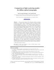
Fig. 1 shows contour plots of the integrated backscattered flux
0
−1
(46)
2π0
F (x, y) = Ψ(µ, ϕ, x, y)µdµdϕ (47)
for various source directions (µ ′ , ϕ ′ ). The source is located 10 ls deep in the half space. The x and y axes are
normalized with respect to ls.
Because the source is not directed normal to the boundary surface in all cases, there is no axi-symmetry.
Fig. 1 shows that the peaks of the integrated fluxes are skewed slightly towards the −ˆx direction. As µ → −1
we observe that the peak of the flux becomes larger and narrower.
In Fig. 2 we show the angular dependence of Ψ evaluated at the origin (x, y) = (8 ls, 8 ls). We show it only
for µ < 0 since imposing the boundary condition yields Ψ = 0 for µ > 0. Fig. 2 shows a non-trivial angular
dependence. The diffusion approximation 1 is used often instead of the transport equation to model light in
tissues. The fundamental assumption in this approximation is that the radiance has become nearly isotropic due
to multiple scattering. Since Fig. 2 shows a significant angular dependence, it indicates that this fundamental
assumption is not valid.
5.2. Asymptotic Result
Suppose that the source is situated deep inside the half space. In that case the contribution from most of the
plane wave modes in (42) and (45) to the point spread function is small. By neglecting all plane wave modes
except for the slowest decaying one, we compute the asymptotic result of the the point spread function as z ′ → ∞.
The Fourier transform of the point spread function defined as
Ψ(ω, 0; κ) = Ψ(ω, ρ, 0)e −iκ·ρ dρ. (48)
R 2
Fourier transforming (37) yields Ψ = G − Y . Because the eigenvalues λj are ordered by their real parts, the
terms in a plane wave mode expansion involving exp[−λ1(κ)z ′ ] in (42) and (45) are the slowest decaying ones
as z ′ → ∞. Neglecting terms involving faster decaying modes yields the asymptotic result
Ψ(ω, 0; κ) ∼ e −λ1(κ)z′
V1(ω ′ ⎡
; κ) ⎣V1(ω; κ) −
⎤
dj,1(κ)Vj(ω; κ) ⎦ , z ′ → ∞. (49)
The coefficients dj,1 are determined from (47) which do not depend on z ′ . The summation term in (49) shows
that the point spread function still maintains a significant amount of directional information. It is because the
radiance must satisfy the boundary condition (36). This directional variation is what is seen in Fig. 2.
j

y
y
20
10
0
−10
−20
20
10
0
−10
−20
−20 −10 0 10 20
x
(a) source direction (µ ′ , ϕ ′ ) = (0.9894, π)
−20 −10 0 10 20
x
(c) source direction (µ ′ , ϕ ′ ) = (−0.7554, π)
−22
−24
−26
−28
−30
−14
−16
−18
−20
−22
−24
−26
y
y
20
10
0
−10
−20
20
10
0
−10
−20
−20 −10 0 10 20
x
(b) source direction (µ ′ , ϕ ′ ) = (0.7554, π)
−20 −10 0 10 20
x
(d) source direction (µ ′ , ϕ ′ ) = (−0.9894, π)
Figure 1. Integrated backscattered flux (47) for various source directions. The optical properties of the medium are given
by σa/σs = 0.01 and g = 0.80. It is for a source at depth z ′ = 10 ls. The x and y axes are normalized by the scattering
mean free path ls. The gray scale of the contours is given in dB.
6. CONCLUSIONS
We have discussed a method to compute the Green’s function for the radiative transport equation. It is given as
an expansion in plane wave modes. These plane wave modes have been calculated numerically using the discrete
ordinate method.
We have used the Green’s function for the radiative transport equation to compute the point spread function
in a half space composed of a uniform scattering and absorbing medium. We have derived an asymptotic result
for the point spread function when the source is deep inside the half space. It shows that the point spread function
has a non-trivial direction dependence. Hence, the fundamental assumption in the diffusion approximation is
not satisifed. Therefore, the diffusion approximation should not be used to compute the point spread function.
ACKNOWLEDGMENTS
The work of A. D. Kim was partially supported by grants AFOSR: F49620-01-1-0465, ONR: N00014-02-1-0088
−20
−22
−24
−26
−28
−12
−14
−16
−18
−20
−22
−24
−26

φ
φ
6
5
4
3
2
1
0
6
5
4
3
2
1
0
−0.8 −0.6 −0.4 −0.2
μ
(a) source direction (µ ′ , ϕ ′ ) = (0.9894, π)
−0.8 −0.6 −0.4 −0.2
μ
(c) source direction (µ ′ , ϕ ′ ) = (−0.7554, π)
−26
−27
−28
−29
−30
−31
−32
−23
−24
−25
−26
−27
−28
−29
−30
φ
φ
6
5
4
3
2
1
0
6
5
4
3
2
1
0
−0.8 −0.6 −0.4 −0.2
μ
(b) source direction (µ ′ , ϕ ′ ) = (0.7554, π)
−0.8 −0.6 −0.4 −0.2
μ
(d) source direction (µ ′ , ϕ ′ ) = (−0.9894, π)
Figure 2. The angular dependence of the radiance at the origin, Ψ(µ, ϕ, 8 ls, 8 ls) at various source angles. All other
parameters are the same as in Fig. 1.
and NSF: DMS-0071578.
REFERENCES
1. A. Ishimaru, Wave Propagation and Scattering in Random Media (New York: IEEE Press, 1996).
2. K. M. Case and P. F. Zweifel, Linear transport theory (Reading, MA: Addison-Wesley, 1967).
3. K. M. Case, “On boundary value problems of linear transport theory,” in Proc. Symp. in Applied Mathematics,
Vol. 1, R. Bellman, G. Birkhoff and I. Abu-Shumays eds., American Mathematical Society 1969,
pp. 17-36.
4. A. D. Kim and J. B. Keller, “Light propagation in biological tissue,” J. Opt. Soc. Am. A 20 92-98 (2003).
5. A. D. Kim, “Transport theory for light propagation in biological tissue,” to appear in J. Opt. Soc. Am. A.
6. K. Atkinson, “Numerical integration on the sphere,” J. Austral. Math. Soc. Ser. B 23 332-347 (1982).
−26
−27
−28
−29
−30
−31
−32
−22
−24
−26
−28
−30