Resolving Ambiguity in Product/Brand Names - SNAP
Resolving Ambiguity in Product/Brand Names - SNAP
Resolving Ambiguity in Product/Brand Names - SNAP

You also want an ePaper? Increase the reach of your titles
YUMPU automatically turns print PDFs into web optimized ePapers that Google loves.
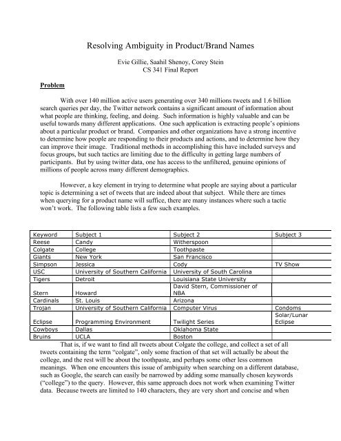
Problem<br />
<strong>Resolv<strong>in</strong>g</strong> <strong>Ambiguity</strong> <strong>in</strong> <strong>Product</strong>/<strong>Brand</strong> <strong>Names</strong><br />
Evie Gillie, Saahil Shenoy, Corey Ste<strong>in</strong><br />
CS 341 F<strong>in</strong>al Report<br />
With over 140 million active users generat<strong>in</strong>g over 340 millions tweets and 1.6 billion<br />
search queries per day, the Twitter network conta<strong>in</strong>s a significant amount of <strong>in</strong>formation about<br />
what people are th<strong>in</strong>k<strong>in</strong>g, feel<strong>in</strong>g, and do<strong>in</strong>g. Such <strong>in</strong>formation is highly valuable and can be<br />
useful towards many different applications. One such application is extract<strong>in</strong>g people’s op<strong>in</strong>ions<br />
about a particular product or brand. Companies and other organizations have a strong <strong>in</strong>centive<br />
to determ<strong>in</strong>e how people are respond<strong>in</strong>g to their products and actions, and to determ<strong>in</strong>e how they<br />
can improve their image. Traditional methods <strong>in</strong> accomplish<strong>in</strong>g this have <strong>in</strong>cluded surveys and<br />
focus groups, but such tactics are limit<strong>in</strong>g due to the difficulty <strong>in</strong> gett<strong>in</strong>g large numbers of<br />
participants. But by us<strong>in</strong>g twitter data, one has access to the unfiltered, genu<strong>in</strong>e op<strong>in</strong>ions of<br />
millions of people across many different demographics.<br />
However, a key element <strong>in</strong> try<strong>in</strong>g to determ<strong>in</strong>e what people are say<strong>in</strong>g about a particular<br />
topic is determ<strong>in</strong><strong>in</strong>g a set of tweets that are <strong>in</strong>deed about that subject. While there are times<br />
when query<strong>in</strong>g for a product name will suffice, there are many <strong>in</strong>stances where such a tactic<br />
won’t work. The follow<strong>in</strong>g table lists a few such examples.<br />
Keyword Subject 1 Subject 2 Subject 3<br />
Reese Candy Witherspoon<br />
Colgate College Toothpaste<br />
Giants New York San Francisco<br />
Simpson Jessica Cody TV Show<br />
USC University of Southern California University of South Carol<strong>in</strong>a<br />
Tigers Detroit Louisiana State University<br />
David Stern, Commissioner of<br />
Stern Howard<br />
NBA<br />
Card<strong>in</strong>als St. Louis Arizona<br />
Trojan University of Southern California Computer Virus Condoms<br />
Solar/Lunar<br />
Eclipse Programm<strong>in</strong>g Environment Twilight Series<br />
Eclipse<br />
Cowboys Dallas Oklahoma State<br />
Bru<strong>in</strong>s UCLA Boston<br />
That is, if we want to f<strong>in</strong>d all tweets about Colgate the college, and collect a set of all<br />
tweets conta<strong>in</strong><strong>in</strong>g the term “colgate”, only some fraction of that set will actually be about the<br />
college, and the rest will be about the toothpaste, and perhaps some other less common<br />
mean<strong>in</strong>gs. When one encounters this issue of ambiguity when search<strong>in</strong>g on a different database,<br />
such as Google, the search can easily be narrowed by add<strong>in</strong>g some manually chosen keywords<br />
(“college”) to the query. However, this same approach does not work when exam<strong>in</strong><strong>in</strong>g Twitter<br />
data. Because tweets are limited to 140 characters, they are very short and concise and when
account<strong>in</strong>g for stop words, spaces, and punctuation, each tweet conta<strong>in</strong>s very few words of<br />
substance from which to determ<strong>in</strong>e the subject matter. Therefore, if one wants to f<strong>in</strong>d tweets<br />
about Reese’s the candy, try<strong>in</strong>g to f<strong>in</strong>d all tweets that conta<strong>in</strong> the words “reese”, “peanut butter”,<br />
and “cups”, there will be very few tweets to look at.<br />
Simply put, our project was aimed at resolv<strong>in</strong>g this ambiguity through automated<br />
processes.<br />
Data<br />
Twitter generously provided us with a very large dataset that conta<strong>in</strong>ed over 3 billion<br />
tweets from late September – late October 2011. In addition to the text of the tweet, other fields<br />
were also provided <strong>in</strong>clud<strong>in</strong>g the date, time, number of followers, and geo-location. In total, the<br />
English language portion of the dataset was approximately 600GB.<br />
Generat<strong>in</strong>g Related Keywords<br />
Our first step <strong>in</strong> try<strong>in</strong>g to determ<strong>in</strong>e a set of tweets about a query term was to f<strong>in</strong>d a set of<br />
related keywords, which we will call “<strong>in</strong>dicator keywords”, as they <strong>in</strong>dicate that the <strong>in</strong>stance of<br />
the query term does <strong>in</strong>deed have the mean<strong>in</strong>g we want.<br />
We <strong>in</strong>itially explored us<strong>in</strong>g tools from the <strong>in</strong>ternet such as Google’s “Related searches”<br />
tool, but found that such methods were <strong>in</strong>effective and did not extend well to tweets. Instead, we<br />
decided to use the texts of the tweets <strong>in</strong> order to generate related search keywords. The measure<br />
we created for rank<strong>in</strong>g possible keywords was developed from our knowledge of association<br />
rules. Specifically, we considered each tweet to be a “basket” of <strong>in</strong>dividual words. Then, given<br />
a target word t, we ranked any possible related keyword k by the follow<strong>in</strong>g similarity measure:<br />
where support(x) means the number of tweets that conta<strong>in</strong> the word x. This measure of similarity<br />
makes sense because if a possible keyword k occurs often with the target word t then they are<br />
more likely to be related, and so the score should <strong>in</strong>crease. Similarly, if k occurs more often<br />
throughout the entire set of tweets, then it is more likely to be a popular word and not necessarily<br />
related to the target word t.<br />
Overall, this measure worked very well and for many products and brand names we were<br />
able to generate a good set of related keywords.<br />
Determ<strong>in</strong><strong>in</strong>g Relevant Keywords: Two Approaches<br />
After devis<strong>in</strong>g a system to come up with relevant keywords, we had to tackle the issue of<br />
determ<strong>in</strong><strong>in</strong>g keywords for terms that were ambiguous. For example, the top fifteen keywords for<br />
Reese were:<br />
witherspoon, toth, pieces, cups, twix, peanut, puffs, kitkats,<br />
butterf<strong>in</strong>gers, butter, snickers, hersheys, kats, twizzlers, skittles
While the first two keywords relate to Reese Witherspoon, the last thirteen are targeted at<br />
the candy (toth refers to Jason Toth, the husband of Reese Witherspoon). We came up<br />
with two ways to resolve this problem.<br />
Method #1: Us<strong>in</strong>g Categories<br />
Our first method relied on the fact that items sometimes belong to specific, well-def<strong>in</strong>ed<br />
categories, and Walmart had given us a well-def<strong>in</strong>ed hierarchy of items that they sold. For<br />
example, Reese’s Peanut Butter Cups clearly belongs to the category of “candy”, and we know<br />
what other items belong to the category of “candy” <strong>in</strong> the Walmart data. Perhaps we could<br />
extract features of the “candy” category, and match our “reese” tweets aga<strong>in</strong>st those features.<br />
The first step was to generate a “master list” of features for a given category. Given a list<br />
of items: {item1, item2, …, itemn} <strong>in</strong> a category, we found all tweets conta<strong>in</strong><strong>in</strong>g any of those item<br />
names. We will call this set of tweets T. Then, we removed stop words and ranked terms present<br />
<strong>in</strong> T by tf-idf. This generated a reasonable list, but we found that some high-rank<strong>in</strong>g words<br />
referred to a s<strong>in</strong>gle item’s other mean<strong>in</strong>g – for example, reese’s non-candy mean<strong>in</strong>g <strong>in</strong>troduced<br />
the term “witherspoon”, which had a high tf-idf and ranked high. In order to downplay<br />
<strong>in</strong>dividual items’ non-candy mean<strong>in</strong>gs, we assigned terms a score of tf-idf *(the number of<br />
dist<strong>in</strong>ct item names they appeared with <strong>in</strong> T).<br />
The second step was to rank the terms occurr<strong>in</strong>g <strong>in</strong> tweets conta<strong>in</strong><strong>in</strong>g the query word<br />
(“reese”) by tf-idf. We separate the top n terms <strong>in</strong> this list (an n of 15 seemed to generally word),<br />
and filter out any words that did not occur <strong>in</strong> the top n*2 terms from the category master list.<br />
This successfully filtered out non-candy terms, but also filtered out some item-specific terms that<br />
only appear <strong>in</strong> one candy. For example, it filtered out “cups” from the “reese” terms, s<strong>in</strong>ce “cup”<br />
only ever occurs.<br />
Method #2: Cluster<strong>in</strong>g Key Words<br />
Although the first method worked well for candies, the assumption that all items will<br />
have as well def<strong>in</strong>ed a category was a strong one and was not easily extendable. However, we<br />
also came up with a second method that works <strong>in</strong> a more general sett<strong>in</strong>g. Our second method<br />
centers around the idea that the keywords that are related to the <strong>in</strong>tended mean<strong>in</strong>g of the query<br />
word will probably be closely related to each other. For example, tak<strong>in</strong>g the top words that cooccur<br />
with “reese”, one would expect that the words “snickers” and “peanut” would be more<br />
closely related to each other than either is to “witherspoon”.<br />
We used jacquard similarity as our notion of similarity. That is, given keywords k1 and<br />
k2, and support(x) mean<strong>in</strong>g the count of tweets conta<strong>in</strong><strong>in</strong>g the term x:<br />
Us<strong>in</strong>g this notion of similarity, we were able to construct an undirected, complete graph with the<br />
nodes represent<strong>in</strong>g the keywords and the edge weight equal<strong>in</strong>g the Jacquard similarity between<br />
the two keywords.
Our plan was to then cluster the nodes of this graph, with the end result hopefully be<strong>in</strong>g<br />
that each cluster would represent a possible mean<strong>in</strong>g of the targeted word. However, all of our<br />
experiments yielded dist<strong>in</strong>ct components. With the number of tweets we considered<br />
(approximately 1 billion English tweets), words like “Snickers” and “Witherspoon” don’t occur<br />
together. S<strong>in</strong>ce the number of words of substance <strong>in</strong> a tweet is so few, unrelated words tend to<br />
occur together either never or very rarely. However, if a larger number of tweets were to be<br />
considered, it would seem that a cluster<strong>in</strong>g method would probably apply.<br />
We tested this method on several different ambiguities and received very positive results.<br />
Outside of Reese, other examples <strong>in</strong>clude “Tigers” and “Stern.” Dur<strong>in</strong>g the timeframe of the<br />
data, the Detroit Tigers were compet<strong>in</strong>g <strong>in</strong> the Major League Baseball Playoffs, while the<br />
Louisiana State University Tigers were the top ranked collegiate football team. When we<br />
applied the cluster<strong>in</strong>g method, to our surprise, we actually had 3 different components: one for<br />
baseball and football, as well as one based on tigers the animal (which <strong>in</strong>cluded words like “lion”<br />
and “cheetah”). For “Stern,” we found two dist<strong>in</strong>ct clusters, one for Howard Stern and one for<br />
David Stern, the commissioner of the National Basketball Association. Although Howard Stern<br />
would generally be considered more famous, dur<strong>in</strong>g the timeframe of our data the NBA was <strong>in</strong> a<br />
lockout, and so David Stern was receiv<strong>in</strong>g a lot of attention on Twitter. The fact that this method<br />
worked towards a product name, a brand name, and a person’s name shows its flexibility and<br />
wide-rang<strong>in</strong>g applicability.<br />
Precision and Recall Us<strong>in</strong>g Method #2<br />
Hav<strong>in</strong>g decided to pursue method #2 over method #1, we next <strong>in</strong>vestigated the trade-offs of<br />
certa<strong>in</strong> parameters, namely n, the number of top co-occurr<strong>in</strong>g words we choose as <strong>in</strong>dicators that<br />
a tweet is about the <strong>in</strong>tended target.<br />
Given a target query “tigers”, we found the top 45 co-occurr<strong>in</strong>g terms for the baseball and<br />
football clusters. We then constructed sets of tweets that each conta<strong>in</strong> “tigers” and any of the top<br />
5 keywords us<strong>in</strong>g method #2 from the baseball or football cluster. We then sampled 100 tweets<br />
out of the result<strong>in</strong>g set and manually recorded how many were about the appropriate team. We<br />
then repeated this process for the top 10, 15, ..., 45 keywords to build a precision/recall graph<br />
12650 tweets <strong>in</strong>cluded “ tigers “<br />
Breakdown (based on random sampl<strong>in</strong>g and a lot of tweet read<strong>in</strong>g):<br />
• 33% Detroit baseball<br />
• 27% LSU football<br />
• 40% neither topic<br />
Detroit Baseball<br />
Number of<br />
Keywords Number of Tweets Precision (%)<br />
5 160 100<br />
10 292 100<br />
15 852 100<br />
20 1630 99
25 2036 99<br />
30 2307 99<br />
35 2823 98<br />
40 2911 98<br />
45 3147 98<br />
LSU Football:<br />
Number of<br />
Keywords Number of Tweets Precision (%)<br />
5 2075 98<br />
10 2196 97<br />
15 2275 97<br />
20 2547 95<br />
25 2723 94<br />
Precision is out of an estimated 4200 tweets<br />
Extensions<br />
Now that we can filter a set of tweets down to only those tweets we are confident are<br />
about the target topic, we can work on expand<strong>in</strong>g our set of tweets. In the methods above, we<br />
always started with the set of tweets conta<strong>in</strong><strong>in</strong>g some keyword, such as “card<strong>in</strong>als”. What if we
could f<strong>in</strong>d all tweets about card<strong>in</strong>als that don’t conta<strong>in</strong> the keyword itself? We did some<br />
prelim<strong>in</strong>ary work with synonym f<strong>in</strong>d<strong>in</strong>g, where<strong>in</strong> we devised the follow<strong>in</strong>g algorithm:<br />
F<strong>in</strong>dSynonyms(W):<br />
T1