Grad, Div, Curl, and all that… - WebRing
Grad, Div, Curl, and all that… - WebRing
Grad, Div, Curl, and all that… - WebRing

You also want an ePaper? Increase the reach of your titles
YUMPU automatically turns print PDFs into web optimized ePapers that Google loves.
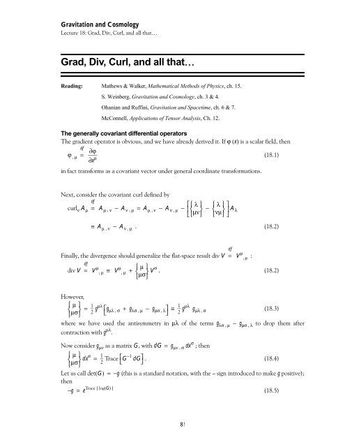
Gravitation <strong>and</strong> Cosmology<br />
Lecture 18: <strong>Grad</strong>, <strong>Div</strong>, <strong>Curl</strong>, <strong>and</strong> <strong>all</strong> <strong>that…</strong><br />
<strong>Grad</strong>, <strong>Div</strong>, <strong>Curl</strong>, <strong>and</strong> <strong>all</strong> <strong>that…</strong><br />
Reading: Mathews & Walker, Mathematical Methods of Physics, ch. 15.<br />
S. Weinberg, Gravitation <strong>and</strong> Cosmology, ch. 3 & 4.<br />
Ohanian <strong>and</strong> Ruffini, Gravitation <strong>and</strong> Spacetime, ch. 6 & 7.<br />
McConnell, Applications of Tensor Analysis, Ch. 12.<br />
The gener<strong>all</strong>y covariant differential operators<br />
The gradient operator is obvious, <strong>and</strong> we have already derived it. If ϕ (x) is a scalar field, then<br />
df<br />
ϕ , μ =<br />
∂ϕ<br />
∂x μ<br />
in fact transforms as a covariant vector under general coordinate transformations.<br />
Next, consider the covariant curl defined by<br />
df<br />
curl ν A μ =<br />
Aμ ; ν − Aν ; μ = Aμ , ν − Aν , μ − ⎡⎧ λ ⎫<br />
⎢⎨ ⎣⎩μν<br />
⎬ −<br />
⎭<br />
⎧ λ ⎫<br />
⎨<br />
⎩νμ<br />
⎬<br />
⎭<br />
⎤ ⎥<br />
⎦<br />
A λ<br />
(18.1)<br />
≡ A μ , ν − A ν , μ . (18.2)<br />
df<br />
Fin<strong>all</strong>y, the divergence should generalize the flat-space result div V =<br />
df<br />
div V =<br />
V μ<br />
; μ<br />
V μ<br />
, μ :<br />
≡ Vμ,<br />
μ + ⎧ μ ⎫<br />
⎨<br />
⎩<br />
μσ<br />
⎬ V<br />
⎭<br />
σ . (18.2)<br />
However,<br />
⎧ μ ⎫<br />
⎨<br />
⎩<br />
μσ<br />
⎬ =<br />
⎭<br />
1<br />
2 gμλ ⎡gμλ , σ + gλσ , μ − gμσ , λ⎤ ≡<br />
⎣ ⎦ 1<br />
2 gμλ gμλ , σ<br />
(18.3)<br />
where we have used the antisymmetry in μλ of the terms g λσ , μ − g μσ , λ to drop them after<br />
contraction with g μλ .<br />
Now consider g μν as a matrix G, with dG = g μν , σ dx σ ; then<br />
⎧ μ ⎫<br />
⎨<br />
⎩<br />
μσ<br />
⎬ dx<br />
⎭<br />
σ = 1<br />
2 Trace ⎡G ⎣ −1 dG⎤ . (18.4)<br />
⎦<br />
Let us c<strong>all</strong> det(G) = −g (this is a st<strong>and</strong>ard notation, with the -- sign introduced to make g positive);<br />
then<br />
−g = e<br />
Trace [ log(G) ]<br />
81<br />
(18.5)
Gravitation <strong>and</strong> Cosmology<br />
The divergence theorem<br />
(Eq. 18.5 is far from obvious, useful, <strong>and</strong> worth remembering. The proof is given below. For now, just<br />
believe it!)<br />
Thus<br />
log(−g) = Tr ⎡ ⎣ log(G)⎤ ⎦<br />
<strong>and</strong><br />
Tr ⎡ ⎣ log(G + dG)⎤ ⎦ = Tr [log(G)] + Tr ⎡ ⎣ log(1 + G −1 dG)⎤ ⎦ ,<br />
hence<br />
log⎛−g − dg⎞ = log⎛−g⎞ + Tr ⎡G ⎝ ⎠ ⎝ ⎠ ⎣ −1 dG⎤<br />
⎦<br />
so that<br />
⎧ μ ⎫<br />
⎨<br />
⎩<br />
μσ<br />
⎬ dx<br />
⎭<br />
σ = 1<br />
2 d ⎡ ⎣ log(−g)⎤ ⎦ ≡ d ⎡ ⎣ log(√⎺⎺−g) ⎤ ⎦<br />
or (we can now drop the -- sign from √⎺⎺−g)<br />
⎧ μ ⎫<br />
⎨<br />
⎩μσ<br />
⎬ = ∂σ log(√⎺g ) =<br />
⎭<br />
1<br />
√⎺g ∂σ √⎺g . (18.6)<br />
‘‘So what?’’ you may say, ‘‘I’ve got my own troubles.’’ Here’s what:<br />
Remember Eq. 18.2? Now we may write<br />
V μ<br />
; μ<br />
= Vμ<br />
, μ<br />
+ 1<br />
√⎺g Vμ ∂ μ √⎺g ≡ 1<br />
√⎺g ∂ μ ⎛ ⎝ V μ √⎺g ⎞ ⎠ . (18.7)<br />
That is, the expression for the covariant divergence is charmingly simple.<br />
The divergence theorem<br />
Under coordinate transformations, the volume element changes like<br />
d n x → d n x _ det ⎛∂x ⎜<br />
⎝∂x<br />
_⎞ ⎟<br />
⎠<br />
where det ⎛∂x ⎜<br />
⎝∂x<br />
_⎞ ⎟ isthe Jacobian of the transformation.<br />
⎠<br />
But<br />
_<br />
gμν<br />
= gκλ ∂xκ<br />
∂x _ μ ∂xλ<br />
∂x _ ν<br />
(18.8)<br />
(18.9)<br />
so, using a well-known property of determinants of matrix-products,<br />
det(AB) = det(A) det(B) , (18.10)<br />
we find<br />
_ ⎡<br />
g = g ⎢⎣ det ⎛∂x ⎜<br />
⎝∂x<br />
_⎞⎤ ⎟⎥ ⎠⎦<br />
i.e.<br />
2<br />
(18.11)<br />
√⎺g d n x = √⎺g _ d n x _ . (18.12)<br />
82
Gravitation <strong>and</strong> Cosmology<br />
Lecture 18: <strong>Grad</strong>, <strong>Div</strong>, <strong>Curl</strong>, <strong>and</strong> <strong>all</strong> <strong>that…</strong><br />
In other words, √⎺g d n x is the invariant volume element in a general space of n dimensions.<br />
Now we can transform the volume integral of a divergence into an integral of a vector over a (normal)<br />
hypersurface.<br />
∫ div V √⎺g d n x = ∫ V μ ; μ √⎺g dn x = ∫ d n x ∂ μ ⎛ ⎝ √⎺g V μ ⎞ ⎠ ≡ ∫ dS μ V μ √⎺g . (18.13)<br />
Proof of the theorem about determinants:<br />
We want to prove that for some matrix G,<br />
log [det(G)] = Tr [log(G)] .<br />
Now this is obvious if the matrix is diagonalizable, with eigenvalues g k since then<br />
⎡<br />
log [det(G)] = log<br />
⎢<br />
⎢<br />
⎣<br />
∏<br />
N<br />
k=1<br />
<strong>and</strong><br />
N<br />
Tr [log(G)] = ∑<br />
k=1<br />
g k<br />
log(g k ) .<br />
⎤<br />
⎥<br />
⎥<br />
⎦<br />
≡ N<br />
∑ log(gk )<br />
k=1<br />
We are concerned to prove the theorem more gener<strong>all</strong>y. First, it had better be true that the matrix<br />
df<br />
A =<br />
log(G)<br />
exists (that is, it can be defined, the matrix has no zero eigenvalues, etc. etc.). Assuming this is the<br />
case, let<br />
df<br />
G(λ) =<br />
Now let us define<br />
e λA , G(1) = e A = G .<br />
df<br />
d log [det(G(λ))] =<br />
log [det(G(λ + dλ))] − log [det(G(λ))]<br />
= log [det(G + dG)] − log [det(G)]<br />
= log [det⎛ ⎝ G(1 + G −1 dG)⎞ ⎠ ] − log [det(G)]<br />
= log [det(1 + G −1 dG)] .<br />
Now let us compute the last term:<br />
83
Gravitation <strong>and</strong> Cosmology<br />
Proof of the theorem about determinants:<br />
det(1 + G −1 ⎪1<br />
+ (G<br />
⎪<br />
dG) =<br />
⎪<br />
⎪<br />
−1 dG) 11<br />
(G −1 dG) 21<br />
= ∏<br />
k<br />
To this same order, then,<br />
≈ 1 + ∑<br />
k<br />
(G −1 dG) 31<br />
…<br />
(G −1 dG) 12<br />
1 + (G −1 dG) 22<br />
(G −1 dG) 32<br />
…<br />
⎡ ⎣ 1 + (G −1 dG) kk ⎤ ⎦ + O⎛ ⎝ (G −1 dG) 2 ⎞ ⎠<br />
(G −1 dG) 13<br />
(G −1 dG) 23<br />
1 + (G −1 dG) 33<br />
…<br />
⎛ ⎝ G −1 dG⎞ ⎠kk ≡ 1 + Tr⎛ ⎝ G −1 dG⎞ ⎠ .<br />
d log [det(G(λ))] = log⎡ ⎣ 1 + Tr⎛ ⎝ G −1 dG⎞ ⎠ ⎤ ⎦ = Tr⎛ ⎝ G −1 dG⎞ ⎠<br />
However, since G(λ) = e λA , clearly<br />
dG(λ) = Ae λA dλ<br />
<strong>and</strong> thus<br />
d log [det(G(λ))] = Tr⎛ ⎝ G −1 dG⎞ ⎠ = Tr⎛ ⎝ e −λA A e λA ⎞ ⎠ dλ ≡ Tr(A) dλ ,<br />
giving, by direct integration,<br />
log [det(G(λ))] = λ Tr(A) + constant .<br />
… ⎪<br />
… ⎪<br />
… ⎪<br />
… ⎪<br />
Since both sides must vanish when λ = 0, the constant is zero, giving at last (with λ = 1)<br />
det(G) = exp [Tr(A)] = exp ⎡ ⎣ Tr(log(G))⎤ ⎦ .<br />
84