Chapter 4
Chapter 4
Chapter 4

You also want an ePaper? Increase the reach of your titles
YUMPU automatically turns print PDFs into web optimized ePapers that Google loves.
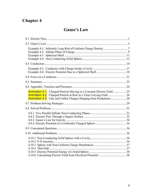
<strong>Chapter</strong> 4<br />
Gauss’s Law<br />
4.1 Electric Flux............................................................................................................. 1<br />
4.2 Gauss’s Law............................................................................................................. 2<br />
Example 4.1: Infinitely Long Rod of Uniform Charge Density ................................ 7<br />
Example 4.2: Infinite Plane of Charge....................................................................... 9<br />
Example 4.3: Spherical Shell................................................................................... 11<br />
Example 4.4: Non-Conducting Solid Sphere........................................................... 13<br />
4.3 Conductors............................................................................................................. 14<br />
Example 4.5: Conductor with Charge Inside a Cavity ............................................ 17<br />
Example 4.6: Electric Potential Due to a Spherical Shell........................................ 18<br />
4.4 Force on a Conductor............................................................................................. 21<br />
4.5 Summary................................................................................................................ 23<br />
4.6 Appendix: Tensions and Pressures ........................................................................ 24<br />
Animation 4.1: Charged Particle Moving in a Constant Electric Field.................. 25<br />
Animation 4.2: Charged Particle at Rest in a Time-Varying Field ........................ 26<br />
Animation 4.3: Like and Unlike Charges Hanging from Pendulums..................... 28<br />
4.7 Problem-Solving Strategies ................................................................................... 29<br />
4.8 Solved Problems .................................................................................................... 31<br />
4.8.1 Two Parallel Infinite Non-Conducting Planes................................................ 31<br />
4.8.2 Electric Flux Through a Square Surface......................................................... 32<br />
4.8.3 Gauss’s Law for Gravity................................................................................. 34<br />
4.8.4 Electric Potential of a Uniformly Charged Sphere ......................................... 34<br />
4.9 Conceptual Questions ............................................................................................ 36<br />
4.10 Additional Problems ............................................................................................ 36<br />
4.10.1 Non-Conducting Solid Sphere with a Cavity................................................ 36<br />
4.10.2 P-N Junction.................................................................................................. 36<br />
4.10.3 Sphere with Non-Uniform Charge Distribution ........................................... 37<br />
4.10.4 Thin Slab....................................................................................................... 37<br />
4.10.5 Electric Potential Energy of a Solid Sphere.................................................. 38<br />
4.10.6 Calculating Electric Field from Electrical Potential ..................................... 38<br />
0
4.1 Electric Flux<br />
Gauss’s Law<br />
In <strong>Chapter</strong> 2 we showed that the strength of an electric field is proportional to the number<br />
of field lines per area. The number of electric field lines that penetrates a given surface is<br />
called an “electric flux,” which we denote as Φ E . The electric field can therefore be<br />
thought of as the number of lines per unit area.<br />
Figure 4.1.1 Electric field lines passing through a surface of area A.<br />
<br />
Consider the surface shown in Figure 4.1.1. Let A = Anˆbe<br />
defined as the area vector<br />
having a magnitude of the area of the surface, A , and<br />
<br />
pointing in the normal direction,<br />
ˆn . If the surface is placed in a uniform electric field E that points in the same direction<br />
as ˆn , i.e., perpendicular to the surface A, the flux through the surface is<br />
<br />
Φ ˆ<br />
E = EA ⋅ = En ⋅ A = EA<br />
(4.1.1)<br />
On the other hand, if the electric field E makes an angle θ with ˆn (Figure 4.1.2), the<br />
electric flux becomes<br />
Φ = EA ⋅ = =<br />
<br />
E EAcosθ En A<br />
<br />
where E = En ⋅ˆis<br />
the component of E perpendicular to the surface.<br />
n<br />
(4.1.2)<br />
Figure 4.1.2 Electric field lines passing through a surface of area A whose normal makes<br />
an angle θ with the field.<br />
1
Note that with the definition for the normal vector ˆn , the electric flux E is positive if<br />
the electric field lines are leaving the surface, and negative if entering the surface.<br />
Φ<br />
In general, a surface S can be curved and the electric field E may vary over the surface.<br />
We shall be interested in the case where the surface is closed. A closed surface is a<br />
surface which completely encloses a volume. In order to compute the electric flux, we<br />
<br />
divide the surface into a large number of infinitesimal area elements ∆ A ˆ<br />
i =∆Aini,<br />
as<br />
shown in Figure 4.1.3. Note that for a closed surface the unit vector nˆ<br />
i is chosen to point<br />
in the outward normal direction.<br />
Figure 4.1.3 Electric field passing through an area element ∆Ai , making an angle θ with<br />
the normal of the surface.<br />
The electric flux through ∆Ai is<br />
<br />
∆Φ = E ⋅∆ A = E∆A cosθ<br />
<br />
E i i i i<br />
(4.1.3)<br />
The total flux through the entire surface can be obtained by summing over all the area<br />
elements. Taking the limit ∆A→0and the number of elements to infinity, we have<br />
<br />
where the symbol<br />
∫∫<br />
S<br />
i<br />
<br />
Φ = lim E ⋅ dA<br />
= E⋅dA (4.1.4)<br />
∑ ∫∫<br />
E i<br />
∆A 0<br />
i<br />
i →<br />
S<br />
denotes a double integral over a closed surface S. In order to<br />
evaluate the above integral, we must first specify the surface and then sum over the dot<br />
<br />
product E⋅dA. 4.2 Gauss’s Law<br />
Consider a positive point charge Q located at the center o f a sphere of radius r, as shown<br />
2<br />
in Figure 4.2.1. The electric field due to the charge Q is E = ( Q/4 πε r ) rˆ<br />
<br />
, which points<br />
0<br />
2
in the radial direction. We enclose the charge by an imaginary sphere of radius r called<br />
the “Gaussian surface.”<br />
Figure 4.2.1 A spherical Gaussian surface enclosing a charge Q .<br />
In spherical coordinates,<br />
a small surface area element on the sphere is given by (Figure<br />
4.2.2)<br />
<br />
2<br />
dA = r sin θ dθ dφ<br />
rˆ<br />
Figure 4.2.2 A small area element on the surface of a sphere of radius r.<br />
Thus, the net electric flux through the area element is<br />
⎛ 1 Q ⎞ 2<br />
Q<br />
dΦ E = E⋅ dA= EdA=⎜ 2 ⎟(<br />
r sin θ dθ dφ) = sin θ dθ dφ<br />
4 0 r 4πε<br />
0<br />
<br />
⎝ πε ⎠<br />
The<br />
total flux through the entire surface is<br />
Q π 2π<br />
Q<br />
Φ E = ∫∫ E⋅ dA= sin θ dθ dφ<br />
=<br />
4πε<br />
∫ ∫ ε<br />
<br />
<br />
S<br />
0 0<br />
0 0<br />
(4.2.1)<br />
(4.2.2)<br />
(4.2.3)<br />
The same result can also be obtained by noting that a sphere of radius<br />
r has a surface area<br />
2<br />
A = 4π<br />
r , and since the magnitude of the electric field at any point on the spherical<br />
2<br />
surface is E = Q/4πε r , the electric flux through the surface is<br />
0<br />
3
E A <br />
⎛ 1 Q ⎞ Q<br />
∫∫ ∫∫<br />
(4.2.4)<br />
2<br />
Φ E = ⋅ d = E dA= EA= ⎜ 4π<br />
r 2 ⎟ =<br />
4πε<br />
S S<br />
0 r ε0<br />
⎝ ⎠<br />
In the above, we have chosen a sphere to be the Gaussian surface. However, it turns out<br />
that the shape of the closed surface can be arbitrarily chosen. For the surfaces shown in<br />
Figure 4.2.3, the same result ( Φ E = Q / ε0<br />
) is obtained. whether the choice is S 1 , 2 or<br />
.<br />
S<br />
S3<br />
Figure 4.2.3 Different Gaussian surfaces with the same outward electric flux.<br />
The statement that the net flux through any closed surface is proportional to the net<br />
charge enclosed is known as Gauss’s law. Mathematically, Gauss’s law is expressed as<br />
q<br />
Φ = ⋅ =<br />
E<br />
enc<br />
∫∫ E dA<br />
(Gauss’s law) (4.2.5)<br />
ε<br />
S<br />
0<br />
where q enc is the net charge inside the surface. One way to explain why Gauss’s law<br />
holds is due to note that the number of field lines that leave the charge is independent of<br />
the shape of the imaginary Gaussian surface we choose to enclose the charge.<br />
To prove Gauss’s law, we introduce the concept of the solid angle. Let 1 1ˆ A<br />
<br />
∆ A =∆ r be<br />
an area element on the surface of a sphere of radius , as shown in Figure 4.2.4.<br />
r<br />
S1 1<br />
Figure 4.2.4 The area element ∆ A subtends a solid angle ∆Ω .<br />
The solid an ∆Ω 1 1ˆ A ∆ A =∆ r<br />
gle subtended by<br />
<br />
at the center of the sphere is defined as<br />
4
∆A<br />
∆Ω ≡ (4.2.6)<br />
r<br />
Solid angles are dimensionless quantities measured in steradians (sr). Since the surface<br />
rea of the sphere is S<br />
2<br />
a 4π r , the total solid angle subtended by the sphere is<br />
1<br />
1<br />
2<br />
1<br />
2<br />
1<br />
1<br />
2<br />
1<br />
4π<br />
r<br />
Ω= = 4π<br />
(4.2.7)<br />
r<br />
The concept of solid angle in three dimensions is analogous to the ordinary angle in two<br />
dimensions. As illustrated in Figure 4.2.5, an angle<br />
∆ ϕ is the ratio of the length of the<br />
arc to the radius r of a circle:<br />
Figure 4.2.5 The arc<br />
s<br />
ϕ<br />
r<br />
∆<br />
∆ = (4.2.8)<br />
∆ s subtends an angle ∆ ϕ .<br />
Since the total length of the arc is s= 2π<br />
r,<br />
the total angle subtended by the circle is<br />
2π<br />
r<br />
ϕ = = 2π<br />
(4.2.9)<br />
r<br />
In Figure 4.2.4, the area element ∆A2 makes an angle θ with the radial unit vector<br />
en the solid angle subtended by A ∆<br />
th is<br />
2<br />
<br />
∆A ⋅rˆ∆A cosθ<br />
∆A<br />
∆Ω = = =<br />
2 2 2n<br />
2<br />
r2 2<br />
r2 2<br />
r2<br />
ˆr ,<br />
(4.2.10)<br />
where 2n 2 cos<br />
A A θ<br />
∆ =∆ is the area of the radial projection of 2 A ∆ onto a s econd sphere S2 of radius r 2 , concentric with S 1 .<br />
As shown in Figure 4.2.4, the solid angle subtended is the same for both ∆A and ∆ A :<br />
1 2n<br />
5
∆A ∆A<br />
cosθ<br />
∆Ω = = (4.2.11)<br />
r r<br />
1 2<br />
2 2<br />
1 2<br />
Now suppose a point charge Q is placed at the center of the concentric spheres. The<br />
electric field strengths at the center of the area<br />
elements 1<br />
oulomb’s law:<br />
A ∆ and 2 A<br />
E1 and E2<br />
∆ are<br />
related by C<br />
1 Q<br />
E i =<br />
4πε<br />
he electric flux through on S1 is A ∆<br />
T<br />
1<br />
E r<br />
⇒ = (4.2.12)<br />
2<br />
2<br />
1<br />
0<br />
2<br />
ri E1 2<br />
r2<br />
∆Φ = E⋅∆ A = E ∆A<br />
<br />
1 1 1<br />
O n the other hand, the electric flux through 2 A ∆ on S2<br />
is<br />
∆Φ = E ⋅ ∆ A = ∆ =<br />
⎛r ⎞ ⎛r ⋅<br />
⎞<br />
= ∆ = Φ<br />
⎝ ⎠ ⎝ ⎠<br />
<br />
2 2<br />
2 2 2 E2 A2cosθ 1 2 E1⎜ 2 ⎟ ⎜ 2 ⎟A1<br />
r2 r1<br />
E1 A1<br />
1<br />
1<br />
(4.2.13)<br />
In summary, Gauss’s law provides a convenient tool for evaluating electric field.<br />
However, its application is limited only to systems that possess certain symmetry,<br />
namely,<br />
systems with cylindrical, planar and spherical symmetry. In the table below, we<br />
give some examples of systems in which Gauss’s law is app licable for determining<br />
electric field, with the c orresponding Gaussian<br />
surfaces:<br />
Symmetry System Gaussian Surface Examples<br />
(4.2.14)<br />
Thus, we see that the electric flux through any area element subtending the same solid<br />
angle is constant, independent of the shape or orientation of the surface.<br />
Cylindrical Infinite rod Coaxial Cylinder Example 4.1<br />
Planar Infinite plane Gaussian “Pillbox” Example 4.2<br />
Spherical Sphere, Spherical shell Concentric Sphere Examples 4.3 & 4.4<br />
The following steps may be useful when applying Gauss’s law:<br />
( 1) Identify the symmetry associated with the charge distribution.<br />
(2) Determine the direction of the electric field, and a “Gaussian surface” on which the<br />
magnitude of the electric field is constant over portions of the surface.<br />
6
(3) Divide the space into different regions associated with the charge distribution. For<br />
each re gion, calculate q , the charge enclosed by the Gaussian surface.<br />
enc<br />
(4) Calculate the electric flux E through the Gaussian surface for each region.<br />
Φ<br />
(5) Equate E Φ with qenc / ε 0 , and deduce the magnitude of the electric field.<br />
Example 4.1: Infinitely Long Rod of Uniform<br />
Charge Density<br />
An infinite ly long rod of negligible radius has a uniform charge density λ . Calculate the<br />
electric field at a distance r from the wire.<br />
Solution:<br />
We shall solve the problem by following the steps outlined above.<br />
(1) An infinitely long rod possesses cylindrical symmetry.<br />
(2) The charge density is uniformly distributed throughout the length,<br />
and the electric<br />
eld E must be point radially away from the symmetry axis of the rod (Figure 4.2.6).<br />
The m gnitude of the electric field is constant on cylindrical surfaces of radius .<br />
Therefore, we choose a coaxial cylinder as our Gaussian surface.<br />
<br />
fi<br />
a r<br />
Figure 4.2.6 Field lines for an infinite uniformly charged rod (the symmetry axis of the<br />
rod and the Gaussian cylinder are perpendicular to plane of the page.)<br />
(3) The amount of charge enclosed by the Gaussian surface, a cylinder of radius r and<br />
length (Figure 4.2.7), is q = λ<br />
.<br />
enc<br />
7
Figure 4.2.7 Gaussian surface for a uniformly charged rod.<br />
(4) As indicated in Figure 4.2.7, the Gaussian surface consists of three parts: a two ends<br />
and plus the curved side wall . The flux through the Gaussian surface is<br />
S<br />
S1 2 S 3<br />
<br />
Φ = E⋅ dA= E ⋅ dA + E ⋅ dA + E ⋅dA<br />
E<br />
∫∫<br />
∫∫ ∫∫ ∫∫<br />
1 1 2 2 3 3<br />
S S1 S2<br />
S3<br />
= 0 + 0 + EA=<br />
E 2π<br />
r<br />
3 3<br />
( )<br />
(4.2.15)<br />
where we have set E3= E.<br />
As can be seen from the figure, no flux passes through the<br />
ends since the area vectors dA1 and dA2 are perpendicular to the electric field which<br />
points in the radial direction.<br />
( 2 π ) = λ/ ε0<br />
(5) Applying Gauss’s law gives E r , or<br />
λ<br />
E = (4.2.16)<br />
2πε<br />
r<br />
The<br />
result is in complete agreement with that obtained in Eq. (2.10.11) using Coulomb’s<br />
law. Notice that the result is independent of the length of the cylinder, an d only<br />
d epends on the inverse of the distance r from the symmetry axis. The qualitative<br />
b ehavior of E as a function of r is plotted in Figure 4.2.8.<br />
Figure 4.2.8 Electric field due to a uniformly charged rod as a function of r<br />
0<br />
8
Example 4.2: Infinite Plane of Charge<br />
Consider<br />
an infinitely large non-conducting plane in the xy-plane with uniform surface<br />
charge<br />
density σ . Determine the electric field everywhere in space.<br />
Solution:<br />
(1) An infinitely large plane possesses a planar symmetry.<br />
(2) Since the charge is uniformly distributed on the surface, the electric field E must<br />
point perpendicularly away from the plane,<br />
<br />
<br />
E= E kˆ.<br />
The magnitude of the electric field<br />
is constant on planes parallel to the non-conducting plane.<br />
Figure 4.2.9 Electric field for uniform plane of charge<br />
We choose our Gaussian surface to be a cylinder, which is often referred to as a “pillbox”<br />
(Figure 4.2.10). The pillbox also consists of three parts: two end-caps and , and a S<br />
curved side . S<br />
3<br />
S1 2<br />
Figure 4.2.10 A Gaussian “pillbox” for calculating the electric field due<br />
to a large plane.<br />
(3)<br />
Since the surface charge distribution on is uniform, the charge enclosed by the<br />
Gaussian “pillbox” is qenc = σ A,<br />
where A= A1 = A2<br />
is the area of the end-caps.<br />
9
(4) The total flux through the Gaussian pillbox flux is<br />
<br />
Φ = E⋅ dA= E ⋅ dA + E ⋅ dA + E ⋅dA<br />
E<br />
∫∫<br />
∫∫ ∫∫ ∫∫<br />
1 1 2 2 3<br />
S S1 S2 S3<br />
= EA+ EA + 0<br />
1 1 2 2<br />
= ( E + E ) A<br />
1 2<br />
3<br />
(4.2.17)<br />
Since the two ends are at the same distance from<br />
the plane, by symmetry, the magnitude<br />
o f the electric field must be the same:<br />
E1 = E2 = E.<br />
Hence,<br />
the total flux can be rewritten<br />
as<br />
(5) By applying Gauss’s law, we obtain<br />
which<br />
gives<br />
In unit-vector notation, we have<br />
2EA<br />
Φ = 2<br />
(4.2.18)<br />
E EA<br />
q σ A<br />
ε ε<br />
enc = =<br />
0 0<br />
σ<br />
E = (4.2.19)<br />
2ε<br />
⎧ σ ˆ<br />
⎪ k,<br />
z > 0<br />
⎪ 2ε<br />
0<br />
E = ⎨<br />
⎪− σ<br />
kˆ<br />
, z < 0<br />
⎪⎩ 2ε<br />
0<br />
0<br />
(4.2.20)<br />
Thus, we see that the electric field due to an infinite large non-conducting plane is<br />
uniform in space. The result, plotted in Figure 4.2.11, is the same as that obtained in Eq.<br />
(2.10.21) using Coulomb’s law.<br />
Figure 4.2.11 Electric field of an infinitely large non-conducting plane.<br />
10
Note again the discontinuity in electric field as we cross the plane:<br />
Example 4.3: Spherical Shell<br />
σ ⎛ σ ⎞ σ<br />
∆ Ez = Ez+ − Ez−<br />
= −⎜− ⎟=<br />
2ε0 ⎝ 2ε0<br />
⎠ ε0<br />
(4.2.21)<br />
A thin spherical shell of radius a has a charge + Q evenly distributed over its surface.<br />
Find<br />
the electric field both inside and outside the shell.<br />
Solutions:<br />
The charge distribution is spherically symmetric, with a surface charge density<br />
2<br />
2<br />
σ = Q/ As= Q/4πa , where As = 4π<br />
a is the surface area of the sphere. The electric field<br />
E must be radially symmetric and directed outward (Figure 4.2.12). We treat the regions<br />
and separately.<br />
<br />
r ≤ a r ≥ a<br />
Case 1:<br />
r ≤ a<br />
Figure 4.2.12 Electric field for uniform spherical shell of charge<br />
We choose our Gaussian surface to be a sphere of radius<br />
4.2.13(a).<br />
(a)<br />
r ≤ a,<br />
as shown in Figure<br />
Figure 4.2.13 Gaussian surface for uniformly charged<br />
spherical shell for (a) r< a,<br />
and<br />
(b ) r ≥ a<br />
(b)<br />
11
T he charge enclosed by the Gaussian surface is q enc = 0 since all the charge is located on<br />
the surface of the shell. Thus, from Gauss’s law, Φ = enc / 0 , we conclude<br />
Case<br />
2:<br />
r ≥ a<br />
E q ε<br />
E = 0, r < a<br />
(4.2.22)<br />
In<br />
this case, the Gaussian surface is a sphere<br />
of radius r ≥ a , as shown in Figure<br />
4.2.13(b).<br />
Since the radius of the “Gaussian sphere” is greater than the radius of the<br />
spherical shell, all the charge is enclosed:<br />
qenc = Q<br />
Since<br />
the flux through the Gaussian surface is<br />
by applying Gauss’s law, we obtain<br />
<br />
2<br />
Φ E = E⋅ dA = EA= E(4 π r )<br />
∫∫<br />
S<br />
Q Q<br />
E = = k , r ≥a<br />
4πε<br />
2 e 2<br />
0r<br />
r<br />
(4.2.23)<br />
Note that the field outside the sphere is the same as if all the charges were concentrated at<br />
the center of the sphere. The qualitative behavior of E as a function of r is plotted in<br />
Figure 4.2.14.<br />
Figure 4.2.14 Electric field as a function of r due to a uniformly charged spherical shell.<br />
As in the case of a non-conducting charged plane, we again see a discontinuity in E as we<br />
cross the boundary at r = a.<br />
The change, from outer<br />
to the inner surface, is given by<br />
Q σ<br />
∆ E = E+ − E−<br />
= − 0 =<br />
4πε<br />
a ε<br />
2<br />
0 0<br />
12
Example 4.4: Non-Conducting Solid Sphere<br />
An electric charge + Q is uniformly distributed throughout a non-conducting solid sphere<br />
of radius a . Determine the electric field everywhere inside and outside the sphere.<br />
Solution:<br />
The charge distribution is spherically symmetric with the charge density given by<br />
Q Q<br />
ρ = =<br />
V (4/3) π a<br />
3<br />
(4.2.24)<br />
<br />
where V is<br />
the volume of the sphere. In this case, the electric field E is radially<br />
symmetric<br />
and directed outward. The magnitude of the electric field is constant on<br />
spherical surfaces of radius r . The regions r ≤ a and r ≥ ashall<br />
be studied separately.<br />
Case 1:<br />
r ≤ a.<br />
We choose our Gaussian surface to be a sphere of radius<br />
4.2.15(a).<br />
(a)<br />
r ≤ a,<br />
as shown in Figure<br />
Figure 4.2.15 Gaussian surface for uniformly charged solid sphere, for (a) r ≤ a,<br />
and (b)<br />
r > a.<br />
The flux through the Gaussian surface is<br />
Φ = E⋅ dA= EA= E π r<br />
<br />
2<br />
(4 )<br />
E<br />
∫∫<br />
With uniform charge distribution,<br />
the charge enclosed is<br />
S<br />
3<br />
⎛ ⎞<br />
⎛43⎞ r<br />
qenc = ∫ ρdV = ρV = ρ⎜ πr<br />
⎟=<br />
Q⎜ 3 ⎟ (4.2.25)<br />
3 a<br />
V<br />
⎝ ⎠ ⎝ ⎠<br />
(b)<br />
13
which is proportional to the volume enclosed by the Gaussian surface. Applying Gauss’s<br />
la Φ = / , we obtain<br />
or<br />
w E qenc ε 0<br />
Case 2 : r ≥ a.<br />
2 ρ ⎛43⎞ E ( 4πr<br />
) = ⎜ πr<br />
⎟<br />
ε ⎝3⎠ 0<br />
0<br />
ρr<br />
Qr<br />
E = = , r ≤ a<br />
(4.2.26)<br />
3<br />
3ε 4πε<br />
a<br />
In this case, our Gaussian surface is a sphere of radius r ≥ a , as shown in Figure<br />
4.2.15(b). Since the radius of the Gaussian surface is greater<br />
than the radius of the sphere<br />
all the charge is enclosed in our Gaussian surface: q = Q.<br />
With the electric flux<br />
2<br />
through the Gaussian surface given by E(4 r ) π Φ = , upon applying Gauss’s law, we<br />
2<br />
obtain E(4 π r ) = Q/<br />
ε , or<br />
0<br />
E<br />
0<br />
2 e 2<br />
0r<br />
r<br />
enc<br />
Q Q<br />
E = = k , r > a<br />
4πε<br />
(4.2.27)<br />
The field outside the sphere is the same as if all the charges were concentrated at the<br />
center of the sphere. The qualitative behavior of E as a function of r is plotted in Figure<br />
4.2.16.<br />
Figure 4.2.16 Electric field due to a uniformly charged sphere as a function of r .<br />
4.3 Conductors<br />
An insulator such as glass or paper is a material in which electrons are attached to some<br />
particular atoms and cannot move freely. On the other hand, inside a conductor, electrons<br />
are free to move around. The basic properties of a conductor are the following:<br />
(1) The electric field is zero inside a conductor.<br />
14
If we place a solid spherical conductor in a constant external field E0 , the positive and<br />
negative charges will move toward the polar<br />
regions of the sphere (the regions on the left<br />
a nd right of the sphere in Figure 4.3.1 below), thereby inducing an electric field E′ .<br />
Inside the conductor, E′ points in the opposite direction of<br />
E0 . Since charges are mobile,<br />
they will continue to move until E′ completely cancels E0 inside the conductor. At<br />
electrostatic equilibrium, E must vanish inside a conductor. Outside the conductor, the<br />
electric field due to the induced charge distribution corresponds to a dipole field, and<br />
the total elec ield is simply<br />
<br />
E′ <br />
<br />
tric f E= E0 + E′<br />
. The field lines are depicted in Figure 4.3.1.<br />
Figure 4.3.1 Placing a conductor in a uniform electric field<br />
(2) Any net charge must reside on the surface.<br />
If there were a net charge inside the conductor, then by Gauss’s law (Eq. 4.3.2), E would<br />
no longer be zero there. Therefore, all the net excess charge must flow to the surface of<br />
the conductor.<br />
<br />
E0 .<br />
Figure 4.3.2 Gaussian surface inside a conductor. The enclosed charge is zero.<br />
ponent of E (3) The tangential com<br />
is zero on the surface of a conductor.<br />
We have already seen that for an isolated conductor, the electric field is zero in its<br />
interior. Any excess charge placed on the conductor must then distribute itself on the<br />
surface, as implied by Gauss’s law.<br />
<br />
Consider the line integral E⋅dsaround a closed path shown in Figure 4.3.3:<br />
∫<br />
15
Figure 4.3.3 Normal and tangential components of electric field outside the conductor<br />
<br />
Since the electric field<br />
E is conservative, the line<br />
integral around the closed path abcda<br />
vanishes:<br />
<br />
∫ E⋅ ds = Et( ∆l) −En( ∆ x') + 0( ∆ l') + En( ∆ x)<br />
= 0<br />
abcda<br />
where Et and En are the tangential and the normal components of the electric field,<br />
respectively, and we have oriented the segment ab so that it is parallel to Et. In the limit<br />
where both ∆x and ∆x'→0, we have Et∆ l = 0. However, since the length element ∆l is<br />
finite,<br />
we conclude that the tangential component of the electric field on the surface of a<br />
conductor<br />
vanishes:<br />
E = 0 (on the surface of a conductor) (4.3.1)<br />
t<br />
This implies that the surface of a conductor in electrostatic equilibrium is an<br />
equipotential<br />
surface. To verify this claim, consider two points A and B on the surface of<br />
a conductor. Since the tangential component E t = 0, the potential difference is<br />
because E is perpendicular to<br />
<br />
VA= VB.<br />
B <br />
V − V =− E⋅ ds<br />
= 0<br />
B A<br />
(4) E is normal to the surface just outside the conductor.<br />
<br />
∫<br />
A<br />
d s . Thus, points A and B are at the same potential with<br />
If the tangential component of E is initially non-zero, charges will then move around<br />
until it vanishes. Hence, only the normal component survives.<br />
16
Figure 4.3.3 Gaussian “pillbox” for computing the electric<br />
field outside the conductor.<br />
To<br />
compute the field strength just outside the conductor, consider the Gaussian pillbox<br />
drawn in Figure 4.3.3. Using Gauss’s law, we obtain<br />
or<br />
A<br />
E d EnA (0) A σ<br />
Φ = ∫∫ E⋅ A=<br />
+ ⋅ =<br />
ε<br />
<br />
(4.3.2)<br />
S<br />
En<br />
0<br />
0<br />
σ<br />
= (4.3.3)<br />
ε<br />
The above result holds for a conductor of arbitrary shape. The pattern of the electric field<br />
line directions for the region near a conductor is shown in Figure 4.3.4.<br />
Figure 4.3.4 Just outside the conductor, E is always perpendicular to the surface.<br />
As in the examples of an infinitely large non-conducting plane and a spherical shell, the<br />
normal component of the electric field exhibits a discontinuity<br />
at the boundary:<br />
( + ) ( −)<br />
σ σ<br />
∆ En = En − En<br />
= − 0 =<br />
ε ε<br />
0 0<br />
Example 4.5: Conductor with Charge Inside a Cavity<br />
17
Consider a hollow conductor shown in Figure 4.3.5 below. Suppose the net charge<br />
carried by the conductor is +Q. In addition, there is a charge q inside the cavity. What is<br />
the charge on the outer surface of the conductor?<br />
Figure 4.3.5 Conductor with a cavity<br />
Since the electric field inside a conductor must be zero, the net charge enclosed by the<br />
Gaussian<br />
surface shown in Figure 4.3.5 must be zero. This implies that a charge –q must<br />
have been induced on the cavity surface. Since the conductor<br />
itself has a charge +Q, the<br />
amount of charge on the outer surface of the conductor must be Q+ q.<br />
Example 4.6: Electric Potential Due to a Spherical Shell<br />
Consider a metallic spherical shell of radius a and charge Q, as shown in Figure 4.3.6.<br />
Figure 4.3.6 A spherical shell of<br />
radius a and charge Q.<br />
(a)<br />
Find the electric potential everywhere.<br />
(b)<br />
Calculate the potential energy of the system.<br />
Solution:<br />
(a)<br />
In Example 4.3, we showed that the electric field for a spherical shell of is given by<br />
18
E <br />
⎧ Q<br />
⎪<br />
4πε<br />
r<br />
rˆ,<br />
r > a<br />
2<br />
= ⎨ 0<br />
⎪ 0, <<br />
⎩<br />
r a<br />
The electric potential may be calculated by using Eq. (3.1.9):<br />
For r > a, we have<br />
B <br />
V − V =− E⋅ds B A<br />
r Q 1 Q<br />
V() r −V( ∞ ) =− ∫ dr′ = = k<br />
∞ 4πε r′ 4πε<br />
r<br />
∫<br />
A<br />
2<br />
0 0<br />
e<br />
Q<br />
r<br />
(4.3.4)<br />
where we have chosen V ( ∞ ) = 0 as our reference point. On the other hand, for r < a, the<br />
potential<br />
becomes<br />
a<br />
r<br />
− ∫ ( ) (<br />
∞ ∫a<br />
V() r V(<br />
∞ ) =− drE r > a − E r < a<br />
a Q 1 Q Q<br />
=− ∫ dr = = k<br />
∞<br />
e<br />
4πε r 4πε<br />
a a<br />
2<br />
0 0<br />
)<br />
(4.3.5)<br />
A plot of the electric potential is shown in Figure 4.3.7. Note that the potential V is<br />
constant inside a conductor.<br />
Figure 4.3.7 Electric potential as a function of r for a spherical conducting shell<br />
(b) The potential energy U can be thought of as the work that needs to be done<br />
to build<br />
up<br />
the system. To charge up the sphere, an external agent must bring charge from infinity<br />
and<br />
deposit it onto the surface of the sphere.<br />
Suppose the charge accumulated on the sphere at some instant is q. The potential at the<br />
su rface of the sphere is then V = q/4πε0a. The amount of work that must be done by an<br />
external agent to bring charge dq from infinity and deposit it on the sphere<br />
is<br />
19
⎛ q ⎞<br />
dWext = Vdq =⎜ ⎟dq<br />
4πε<br />
a<br />
⎝ 0 ⎠<br />
Therefore, the total amount of work needed to charge the sphere to Q is<br />
Since 0<br />
2<br />
Q q Q<br />
Wext = ∫ dq =<br />
0 4πε<br />
a 8πε a<br />
0 0<br />
V = Q/4πε a and Wext = U , the above expression is simplified to<br />
(4.3.6)<br />
(4.3.7)<br />
1<br />
U = QV<br />
(4.3.8)<br />
2<br />
The result can be contrasted with<br />
the case of a point charge. The work required to bring a<br />
point<br />
charge Q from infinity to a point where the electric potential due to other charges is<br />
V would be W = QV<br />
. Therefore, for a point charge Q, the potential energy is U=QV.<br />
ext<br />
Now, suppose two metal spheres with radii r1 and 2 are connected by a thin conducting<br />
wire, as shown in Figure 4.3.8.<br />
r<br />
Figure 4.3.8 Two conducting spheres connected by a wire.<br />
Charge will continue to flow until equilibrium is established such<br />
that both spheres are at<br />
e same potential V1 = V2 = V.<br />
Suppose the charges on the spheres at equilibrium are 1<br />
. Neglecting the effect of the wire that connects the two spheres, the equipotential<br />
ondition implies<br />
q<br />
th<br />
and q2<br />
c<br />
1 q1 1 q2<br />
V = =<br />
4πε r 4πε<br />
r<br />
or<br />
0 1 0 2<br />
q1 q2<br />
= (4.3.9)<br />
r r<br />
1 2<br />
assuming<br />
that the two spheres are very far apart so that the charge distributions on the<br />
surfaces of the conductors are uniform. The electric fields can be expressed as<br />
20
1 q σ 1 q σ<br />
E = = , E = = (4.3.10)<br />
1 1 2 2<br />
1 2<br />
4πε0<br />
r1 ε0<br />
2<br />
2<br />
4πε0 r2<br />
ε0<br />
w here σ 1 and σ 2 are the surface charge densities on spheres 1 and 2, respectively. The<br />
two equations can be combined to yield<br />
E1 σ1<br />
r2<br />
= = (4.3.11)<br />
E σ r<br />
2 2 1<br />
With<br />
the surface charge density<br />
being inversely proportional to the radius, we conclude<br />
that the regions with the smallest radii of curvature have the greatest σ . Thus, the<br />
electric field strength on the surface of a conductor is greatest at the sharpest point. The<br />
design of a lightning rod is based on this principle.<br />
4.4 Force on a Conductor<br />
We have seen that at the boundary surface of a conductor with a uniform charge density<br />
σ, the tangential component of the electric field is zero, and hence, continuous, while the<br />
normal component of the electric field exhibits discontinuity, with ∆ En = σ / ε 0 . Consider<br />
a small patch of charge on a conducting surface, as shown in Figure 4.4.1.<br />
Figure 4.4.1 Force on a conductor<br />
What is the force experienced by this patch? To answer this question, let’s write the total<br />
electric field anywhere outside the surface as<br />
where<br />
E <br />
patch<br />
<br />
E=E E<br />
(4.4.1)<br />
′<br />
patch +<br />
is the electric field due to charge on the patch, and ′<br />
E is the electric field due<br />
to all other charges. Since by Newton’s third law, the patch<br />
cannot exert a force on itself,<br />
the force on the patch m ust come solely from E′ . Assuming the patch to be a flat surface,<br />
from Gauss’s law, the electric field due to the patch is<br />
21
E <br />
patch<br />
⎧ σ ˆ<br />
⎪<br />
+ k,<br />
z > 0<br />
⎪ 2ε<br />
0<br />
= ⎨<br />
⎪ σ<br />
− kˆ<br />
, z < 0<br />
⎪⎩ 2ε<br />
0<br />
By superposition principle, the electric field above the conducting<br />
surface is<br />
⎛ σ ⎞ <br />
E ˆ ′<br />
above = ⎜ ⎟k+<br />
E<br />
2ε<br />
⎝ 0 ⎠<br />
Similarly, below the conducting<br />
surface, the electric field is<br />
⎝ 0 ⎠<br />
(4.4.2)<br />
(4.4.3)<br />
⎛ σ ⎞ <br />
E ˆ ′<br />
below = − ⎜ ⎟k+<br />
E<br />
(4.4.4)<br />
2ε<br />
<br />
Notice<br />
that E′<br />
is continuous across the boundary. This is due to the fact that if the patch<br />
were<br />
removed, the field in the remaining “hole” exhibits no discontinuity. Using the two<br />
equations<br />
above, we find<br />
1 <br />
E′ = ( E + E ) =E<br />
2<br />
above below avg<br />
<br />
the case of a conductor, with E = ( σ / ε ) k and E <br />
In = 0 , we have<br />
Thus, the force acting on the patch is<br />
above 0 ˆ<br />
below<br />
(4.4.5)<br />
1 ⎛σ ˆ<br />
⎞ σ<br />
E ˆ<br />
avg = ⎜ k + 0⎟=<br />
k (4.4.6)<br />
2⎝ε0 ⎠ 2ε0<br />
<br />
2<br />
σ ˆ σ A<br />
F= qE ˆ<br />
avg = ( σ A) k = k<br />
2ε 2ε<br />
0 0<br />
(4.4.7)<br />
where A is the area of the patch. This is precisely the force needed<br />
to drive the charges<br />
on the surface of a conductor to an equilibrium state where the electric field just outside<br />
the conductor takes on the value σ / ε and vanishes inside. Note that irrespective of the<br />
sign of σ, the force tends to pull the patch into the field.<br />
0<br />
Using<br />
the result obtained above, we may define the electrostatic pressure on the patch as<br />
22
2<br />
2<br />
F σ 1 ⎛σ ⎞ 1<br />
ε0⎜ ⎟ ε0<br />
A 2ε0 2 ε0<br />
2<br />
P = = = = E<br />
⎝ ⎠<br />
2<br />
(4.4.8)<br />
where<br />
E is the magnitude of the field just above the patch. The pressure is being<br />
transmitted<br />
via the electric field.<br />
4.5 Summary<br />
• The electric flux that passes through a surface<br />
characterized by the area vector<br />
<br />
A = Anˆis<br />
Φ E = EA ⋅ = EAcosθ <br />
where θ is the angle between the electric field E and the unit vector ˆn .<br />
• In general, the electric flux through a surface is<br />
Φ = E⋅ A<br />
<br />
∫∫<br />
E d<br />
S<br />
• Gauss’s law states that the electric flux through any closed Gaussian surface is<br />
proportional<br />
to the total charge enclosed by the surface:<br />
q<br />
Φ E = ∫∫ E⋅ dA=<br />
ε<br />
S<br />
Gauss’s law can be used to calculate the electric field for a system that possesses<br />
planar, cylindrical or spherical symmetry.<br />
• The normal component of the electric field exhibits discontinuity, with<br />
∆ E = σ / ε , when crossing a boundary with surface charge density σ.<br />
n<br />
0<br />
• The basic properties of a conductor are (1) The electric field inside a conductor is<br />
zero; (2) any net charge must reside on the surface of the conductor; (3) the<br />
surface of a conductor is an equipotential surface, and the tangential component<br />
of the electric field on the surface is zero; and (4) just outside the conductor, the<br />
electric field is normal to the surface.<br />
• Electrostatic pressure on a conducting surface is<br />
enc<br />
0<br />
23
4.6 Appendix: Tensions and Pressures<br />
2<br />
2<br />
σ 1 ⎛σ ⎞ 1<br />
ε0⎜ ⎟ ε0<br />
2ε0 2 ε0<br />
2<br />
F<br />
P = = = = E<br />
A<br />
⎝ ⎠<br />
In Section 4.4, the pressure transmitted by the electric field on a conducting surface was<br />
derived. We now consider a more general case where a closed surface (an imaginary box)<br />
is placed in an electric field, as shown in Figure 4.6.1.<br />
If we look at the top face of the imaginary box, there is an electric field pointing in the<br />
outward<br />
normal direction of that<br />
face. From Faraday’s field theory perspective, we would<br />
say<br />
that the field on that face transmits a tension along itself across the face, thereby<br />
resulting in an upward pull, just as if we had attached a string under tension to that face<br />
to pull it upward. Similarly, if we look at the bottom face of the imaginary box, the field<br />
on that face is anti-parallel to the outward normal of the face, and according to Faraday’s<br />
interpretation, we would again say that the field on the bottom face transmits a tension<br />
along itself, giving rise to a downward pull, just as if a string has been attached to that<br />
face to pull it downward. (The actual determination of the direction of the force requires<br />
an advanced treatment using the Maxwell’s stress tensor.) Note that this is a pull parallel<br />
to the outward normal of the bottom face, regardless of whether the field is into the<br />
surface or out of the surface.<br />
Figure 4.6.1 An imaginary box in an electric field (long orange vectors). The short<br />
vectors indicate the directions of stresses transmitted by the field, either pressures (on the<br />
left or right faces of the box) or tensions (on the top and bottom faces of the box).<br />
For the left side of the imaginary box, the field on that face is perpendicular to the<br />
outward normal of that face, and Faraday would have said that the field on that face<br />
transmits a pressure perpendicular to itself, causing a push to the right. Similarly, for the<br />
right side of the imaginary box, the field on that face is perpendicular to the outward<br />
normal<br />
of the face, and the field would transmit a pressure perpendicular to itself. In this<br />
case, there is a push to the left.<br />
2<br />
24
Note that the term “tension” is used when the stress transmitted by the field is parallel (or<br />
anti-parallel) to the outward normal of the surface, and “pressure” when it is<br />
perpendicular to the outward normal. The magnitude of these pressures and tensions on<br />
2<br />
the<br />
various faces of the imaginary surface in Figure 4.6.1 is given by ε 0 E /2 for the<br />
electric field. This quantity has units of force per unit area, or pressure. It is also the<br />
energy density stored in the electric field since energy per unit volume has the<br />
same units<br />
as pressure.<br />
Animation 4.1:<br />
Charged Particle Moving in a Constant Electric Field<br />
As an example of the stresses transmitted<br />
by electric fields, and of the interchange of<br />
e nergy between fields and particles, consider a positive electric charge q > 0 moving in a<br />
constant electric field.<br />
Suppose the charge is initially moving upward along the positive z-axis in a constant<br />
background field 0 . Since the charge experiences a constant downward force<br />
k, it eventually comes to rest (say, at the origin z = 0), and then moves<br />
back down the negative z-axis. motion and the fields that accompany it are shown<br />
Figure 4.6.2, at two different t .<br />
ˆ<br />
<br />
E=−E k<br />
0 ˆ<br />
<br />
Fe= qE=−qE This<br />
in<br />
imes<br />
(a) (b)<br />
Figure 4.6.2 A positive charge moving in a constant electric field which points<br />
downward. (a) The total field configuration when the charge is still out of sight on the<br />
negative z-axis. (b) The total field configuration when the charge comes to rest at the<br />
origin, before it moves back down the negative z-axis.<br />
How do we interpret the motion of the charge in terms of the stresses transmitted by the<br />
fields? Faraday would have described the downward force on the charge in Figure<br />
4.6.2(b) as follows: Let the charge be surrounded by an imaginary sphere centered on it,<br />
as shown in Figure 4.6.3. The field lines piercing the lower half of the sphere transmit a<br />
tension that is parallel to the field. This is a stress pulling downward on the charge from<br />
below. The field lines draped over the top of the imaginary sphere transmit a pressure<br />
perpendicular to themselves. This is a stress pushing down on the charge from above. The<br />
total effect of these stresses is a net downward force on the charge.<br />
25
Figure 4.6.3 An electric charge in a constant downward electric field. We surround the<br />
charge by an imaginary sphere in order to discuss the stresses transmitted across the<br />
surface of that sphere by the electric field.<br />
Viewing the animation of Figure 4.6.2 greatly enhances Faraday’s interpretation of the<br />
stresses in the static image. As the charge moves upward, it is apparent in the animation<br />
that the electric field lines are generally compressed above the charge and stretched<br />
below the charge. This field configuration enables the transmission of a downward force<br />
to the moving charge we can see as well as an upward force to the charges that produce<br />
the constant field, which we cannot see. The overall appearance of the upward motion of<br />
the charge through the electric field is that of a point being forced into a resisting<br />
m edium,<br />
with stresses arising in that medium as a result of that encroachment.<br />
The kinetic energy of the upwardly moving charge is decreasing as more and more<br />
energy is stored in the compressed electrostatic field, and conversely when the charge is<br />
moving downward. Moreover, because the field line motion in the animation is in the<br />
direction of the energy flow, we can explicitly see the electromagnetic energy flow away<br />
from the charge into the surrounding field when the charge is slowing. Conversely, we<br />
see the electromagnetic energy flow back to the charge from the surrounding field when<br />
the charge is being accelerated back down the z-axis by the energy released from the<br />
field.<br />
Finally, consider momentum conservation. The moving charge in the animation of<br />
Figure<br />
4.6.2 completely reverses its direction of motion over the course of the animation.<br />
How do we conserve momentum in this process? Momentum is conserved because<br />
momentum in the positive z-direction is transmitted from the moving charge to the<br />
charges that are generating the constant downward electric field (not shown). This is<br />
obvious<br />
from the field configuration shown in Figure 4.6.3. The field stress, which<br />
pushes downward on the charge, is accompanied<br />
by a stress pushing upward on the<br />
charges<br />
generating the constant field.<br />
Animation 4.2: Charged Particle at Rest in a Time-Varying Field<br />
As a second example of the stresses transmitted by electric fields, consider a positive<br />
point charge sitting at rest at the origin in an external field which is constant in space but<br />
varies in time. This external field is uniform varies according to the equation<br />
26
4 ⎛2πt⎞ E=−E ˆ<br />
0 sin ⎜ ⎟k<br />
⎝ T ⎠<br />
(a) (b)<br />
(4.6.1)<br />
Figure 4.6.4 Two frames of an animation of the electric field around a positive charge<br />
sitting at rest in a time-changing electric field that points downward. The orange vector<br />
is the electric field and the white vector is the force on the point charge.<br />
Figure 4.6.4 shows two frames of an animation of the total electric field configuration for<br />
this situation. Figure 4.6.4(a) is at t = 0, when the vertical electric field is zero. Frame<br />
4.6.4(b) is at a quarter period later, when the downward electric field is at a maximum.<br />
As<br />
in Figure 4.6.3 above, we interpret the field configuration in Figure 4.6.4(b) as<br />
indicating a net downward force on the stationary charge. The animation of Figure 4.6.4<br />
shows dramatically the inflow of energy into the neighborhood of the charge as the<br />
external electric field grows in time, with a resulting build-up of stress that transmits a<br />
downward force to the positive charge.<br />
We<br />
can estimate the magnitude of the force on the charge in Figure 4.6.4(b) as follows.<br />
At the time shown in Figure 4.6.4(b), the distance<br />
r 0 above the charge at which the<br />
electric field of the charge is equal and opposite to the constant electric field is<br />
determined<br />
by the equation<br />
E<br />
q<br />
= (4.6.2)<br />
0 2<br />
4πε0r0<br />
2<br />
The surface area of a sphere of this radius is A = 4 π r0 = q/ ε 0E0.<br />
Now according to Eq.<br />
(4.4.8) the pressure (force per unit area) and/or<br />
tension transmitted across the surface of<br />
2<br />
this<br />
sphere surrounding<br />
the charge is of the order of ε E /2.<br />
Since the electric field on<br />
the surface of the sphere is of order E 0 , the total force transmitted by the field is of order<br />
2<br />
2 2 2<br />
ε 0E0 /2 times the area of the sphere, or ( ε0E0 /2)(4 πr0 ) = ( ε0E0 /2)( q/ ε0E0)<br />
≈ qE0,<br />
as<br />
we expect.<br />
Of course this net force is a combination of a pressure pushing down on the top of the<br />
sphere and a tension pulling down across the bottom of the sphere. However, the rough<br />
estimate that we have just made demonstrates that the pressures and tensions transmitted<br />
0<br />
27
2<br />
across the surface of this sphere surrounding the charge are plausibly of order ε 0 E /2,<br />
as<br />
we claimed in Eq. (4.4.8).<br />
Animation 4.3: Like and Unlike Charges Hanging from Pendulums<br />
Consider two charges hanging from pendulums whose supports can be moved closer or<br />
further<br />
apart by an external agent. First, suppose the charges both have the same sign,<br />
and therefore repel.<br />
Figure 4.6.5 Two pendulums from which are suspended charges of the same sign.<br />
Figure 4.6.5 shows the situation when an external agent tries to move the supports (from<br />
which the two positive charges are suspended) together. The force of gravity is pulling<br />
the charges down, and the force of electrostatic repulsion is pushing them apart on the<br />
radial line joining them. The behavior of the electric fields in this situation is an example<br />
of an electrostatic pressure transmitted perpendicular to the field. That pressure tries to<br />
keep the two charges apart in this situation, as the external agent controlling the<br />
pendulum supports tries to move them together. When we move the supports together the<br />
charges are pushed apart by the pressure transmitted perpendicular to the electric field.<br />
We artificially terminate the field lines at a fixed distance from the charges to avoid<br />
visual confusion.<br />
In contrast, suppose the charges are of opposite signs, and therefore attract. Figure 4.6.6<br />
shows the situation when an external agent moves the supports (from which the two<br />
positive charges are suspended) together. The force of gravity is pulling the charges<br />
down, and the force of electrostatic attraction is pulling them together on the radial line<br />
joining them. The behavior<br />
of the electric fields in this situation is an example of the<br />
tension<br />
transmitted parallel to the field. That tension tries to pull the two unlike charges<br />
together in this situation.<br />
Figure 4.6.6 Two pendulums with suspended charges of opposite sign.<br />
28
When we move the supports together the charges are pulled together by the tension<br />
transmitted<br />
parallel to the electric field. We artificially terminate the field lines at a fixed<br />
distance<br />
from the charges to avoid visual confusion.<br />
4.7 Problem-Solving Strategies<br />
In this chapter, we have shown how electric field can be computed using Gauss’s law:<br />
qenc<br />
Φ E = ∫∫ E⋅ dA<br />
=<br />
ε<br />
S<br />
The procedures are outlined in Section 4.2. Below we summarize how the above<br />
procedures can be employed to compute the electric field for a line of charge, an infinite<br />
plane of charge and a uniformly charged solid sphere.<br />
0<br />
29
System<br />
Figure<br />
Identify the<br />
symmetry<br />
Determine the<br />
direction of E <br />
Divide the space<br />
into different<br />
regions<br />
Choose Gaussian<br />
surface<br />
Calculate electric<br />
flux<br />
Calculate enclosed<br />
charge<br />
q<br />
in<br />
Apply Gauss’s law<br />
Φ = to<br />
E qin / ε 0<br />
find E<br />
Infinite line of<br />
charge<br />
Infinite plane of<br />
charge<br />
Uniformly charged<br />
solid sphere<br />
Cylindrical Planar Spherical<br />
r > 0<br />
z > 0 and z < 0 r ≤ a and r ≥ a<br />
Coaxial cylinder<br />
Gaussian pillbox<br />
Concentric sphere<br />
E(2 rl)<br />
π Φ = EA EA 2EA<br />
Φ = + = 2<br />
E(4 r ) π Φ =<br />
E<br />
q l<br />
enc = λ<br />
enc<br />
λ<br />
E =<br />
2πε<br />
r<br />
0<br />
E<br />
q = σ A<br />
σ<br />
E =<br />
2ε<br />
0<br />
q<br />
enc<br />
E<br />
3<br />
⎧Qr<br />
( / a) r≤a = ⎨<br />
⎩Q<br />
r≥a<br />
⎧ Qr<br />
⎪<br />
, r≤a 3<br />
⎪4πε0a<br />
E = ⎨<br />
⎪ Q<br />
, r≥a 2 ⎪⎩ 4πε0r<br />
30
4.8 Solved Problems<br />
4.8.1 Two Parallel Infinite Non-Conducting Planes<br />
Two parallel infinite non-conducting planes lying in the xy-plane are separated by a<br />
distance d . Each plane is uniformly charged with equal but opposite surface charge<br />
densities, as shown in Figure 4.8.1. Find the electric field everywhere in space.<br />
Solution:<br />
Figure 4.8.1 Positive and negative uniformly charged infinite planes<br />
The electric field due to the two planes can be found by applying the superposition<br />
principle to the result obtained in Example 4.2 for one plane. Since the planes carry equal<br />
but opposite surface charge densities, both fields have equal magnitude:<br />
σ<br />
E+ = E−<br />
=<br />
2ε<br />
The field of the positive plane points away from the positive plane and the field of the<br />
negative plane points towards the negative plane (Figure 4.8.2)<br />
Figure 4.8.2 Electric field of positive and negative planes<br />
Therefore, when we add these fields together, we see that the field outside the parallel<br />
planes is zero, and the field between the planes has twice the magnitude of the field of<br />
either plane.<br />
0<br />
31
Figure 4.8.3 Electric field of two parallel planes<br />
The electric field of the positive and the negative planes are given by<br />
⎧ σ ˆ ⎧ σ<br />
, /2 ˆ<br />
⎪<br />
+ k z > d , z d<br />
2ε ⎪<br />
− k >− /2<br />
⎪ 0<br />
⎪ 2ε0<br />
E+ = ⎨ , E−<br />
= ⎨<br />
⎪ σ ˆ σ<br />
− k, z< d/2 ⎪+<br />
kˆ,<br />
z d/2<br />
⎪<br />
⎪ σ<br />
E= ⎨−<br />
kˆ<br />
, d/2 > z >−d/<br />
2 (4.8.1)<br />
⎪ ε 0<br />
⎪<br />
⎩0<br />
kˆ<br />
, z d /2and<br />
z < − d /2.<br />
4.8.2 Electric Flux Through a Square Surface<br />
(a) Compute the electric flux through a square surface of edges 2l due to a charge +Q<br />
located at a perpendicular distance l from the center of the square, as shown in Figure<br />
4.8.4.<br />
Figure 4.8.4 Electric flux through a square surface<br />
32
(b) Using the result obtained in (a), if the charge +Q is now at the center of a cube of side<br />
2l (Figure 4.8.5), what is the total flux emerging from all the six faces of the closed<br />
surface?<br />
Solutions:<br />
Figure 4.8.5 Electric flux through the surface of a cube<br />
(a) The electric field due to the charge +Q is<br />
1 Q 1 Q ⎛ xˆi+ yˆj+<br />
zkˆ⎞<br />
E ˆr=<br />
= 2 2 ⎜ ⎟<br />
4πε0 r 4πε0<br />
r ⎝ r ⎠<br />
2 2 2 1/ 2<br />
where r = ( x + y + z ) in Cartesian coordinates. On the surface S, y = l and the area<br />
<br />
element is dA = dAˆj= ( dxdz)j<br />
ˆ . Since ˆˆ i⋅j= ˆj⋅ kˆ = 0and<br />
ˆˆ j⋅ j= 1,<br />
we have<br />
Q ⎛ xˆi+ yˆj+ zkˆ⎞ Ql<br />
E⋅ dA= ( dxdz)<br />
ˆ<br />
2 ⎜ ⎟⋅<br />
j=<br />
4πε0r ⎝ r ⎠ 4πε0r<br />
Thus, the electric flux through S is<br />
3 dxdz<br />
Ql l l dz Ql l<br />
z<br />
Φ = ∫∫<br />
E⋅ dA= ∫ dx∫= ∫ dx<br />
( x + l )( x + l + z )<br />
E 2 2 2 3/ 2<br />
4 πε −l −l<br />
2 2 2 2 2 1 2<br />
0 ( x + l + z ) 4πε<br />
−l<br />
/<br />
S<br />
0<br />
Ql l l dx Q ⎛ 1 x ⎞<br />
−<br />
= 2 2 2 2 1/2 tan<br />
2 πε ∫<br />
= ⎜ ⎟<br />
−l<br />
2 2<br />
0 ( x + l )( x + 2 l ) 2πε⎜ ⎟<br />
0 ⎝ x + 2l<br />
⎠<br />
Q −1 −1<br />
Q<br />
= ⎡tan (1 / 3) tan ( 1/ 3) ⎤<br />
2πε ⎣<br />
− −<br />
⎦<br />
=<br />
6ε<br />
0 0<br />
where the following integrals have been used:<br />
l<br />
−l<br />
l<br />
−l<br />
33
∫<br />
∫<br />
dx x<br />
=<br />
( x + a ) a ( x + a )<br />
2 2 3/2 2 2 2 1/2<br />
dx 1<br />
b a<br />
( x + a )( x + b ) a( b − a ) a ( x + b )<br />
2 2<br />
−1<br />
− 2 2<br />
= tan , b > a<br />
2 2 2 2 1/2 2 2 1/2 2 2 2<br />
(b) From symmetry arguments, the flux through each face must be the same. Thus, the<br />
total flux through the cube is just six times that through one face:<br />
⎛ Q ⎞ Q<br />
Φ E = 6⎜ ⎟=<br />
⎝ 6ε0<br />
⎠ ε0<br />
The result shows that the electric flux Φ E passing through a closed surface is<br />
proportional to the charge enclosed. In addition, the result further reinforces the notion<br />
that ΦE<br />
is independent of the shape of the closed surface.<br />
4.8.3 Gauss’s Law for Gravity<br />
What is the gravitational field inside a spherical shell of radius a and mass m ?<br />
Solution:<br />
Since the gravitational force is also an inverse square law, there is an equivalent Gauss’s<br />
law for gravitation:<br />
Φ =− 4π<br />
Gm<br />
(4.8.2)<br />
g<br />
The only changes are that we calculate gravitational flux, the constant 1/ ε 0 →− 4πG ,<br />
and qenc → menc.<br />
For r ≤ a,<br />
the mass enclosed in a Gaussian surface is zero because the<br />
mass is all on the shell. Therefore the gravitational flux on the Gaussian surface is zero.<br />
This means that the gravitational field inside the shell is zero!<br />
4.8.4 Electric Potential of a Uniformly Charged Sphere<br />
An insulated solid sphere of radius a has a uniform charge density ρ. Compute the<br />
electric potential everywhere.<br />
Solution:<br />
enc<br />
34
Using Gauss’s law, we showed in Example 4.4 that the electric field due to the charge<br />
distribution is<br />
⎧ Q<br />
⎪ rˆ,<br />
r > a<br />
2<br />
⎪ 4πε0r<br />
E = ⎨<br />
⎪ Qr<br />
rˆ,<br />
r < a<br />
3 ⎪⎩ 4πε0a<br />
Figure 4.8.6<br />
The electric potential at P1<br />
(indicated in Figure 4.8.6) outside the sphere is<br />
r Q 1 Q<br />
V () r −V( ∞ ) =− ∫ dr′ = = k<br />
r′ r<br />
1<br />
∞<br />
2<br />
4πε0 4πε0<br />
On the other hand, the electric potential at P2<br />
inside the sphere is given by<br />
( ) ( )<br />
2<br />
∞ a ∞<br />
2 3<br />
4πε a<br />
0r 4πε<br />
0a<br />
2 ⎛ ⎞<br />
e<br />
2 ⎛ ⎞<br />
(4.8.3)<br />
Q<br />
r (4.8.4)<br />
a r a Q r Qr<br />
V () r −V( ∞ ) =− drE r > a − E r < a =− dr − dr′ r′<br />
∫ ∫ ∫ ∫<br />
1 Q 1 Q 1 2 2 1 Q r<br />
= − 3 ( r − a ) = ⎜3− 2 ⎟<br />
4πε 0 a 4πε 0 a 2 8πε<br />
0 a ⎝ a ⎠<br />
Q r<br />
= ke<br />
⎜3− 2 ⎟<br />
2a⎝<br />
a ⎠<br />
A plot of electric potential as a function of r is given in Figure 4.8.7:<br />
Figure 4.8.7 Electric potential due to a uniformly charged sphere as a function of r.<br />
(4.8.5)<br />
35
4.9 Conceptual Questions<br />
1. If the electric field in some region of space is zero, does it imply that there is no<br />
electric charge in that region?<br />
2. Consider the electric field due to a non-conducting infinite plane having a uniform<br />
charge density. Why is the electric field independent of the distance from the plane?<br />
Explain in terms of the spacing of the electric field lines.<br />
3. If we place a point charge inside a hollow sealed conducting pipe, describe the<br />
electric field outside the pipe.<br />
4. Consider two isolated spherical conductors each having net charge Q > 0 . The<br />
spheres have radii a and b, where b>a. Which sphere has the higher potential?<br />
4.10 Additional Problems<br />
4.10.1 Non-Conducting Solid Sphere with a Cavity<br />
A sphere of radius 2R is made of a non-conducting material that has a uniform volume<br />
charge density ρ . (Assume that the material does not affect the electric field.) A<br />
spherical cavity of radius R is then carved out from the sphere, as shown in the figure<br />
below. Compute the electric field within the cavity.<br />
4.10.2 P-N Junction<br />
Figure 4.10.1 Non-conducting solid sphere with a cavity<br />
When two slabs of N-type and P-type semiconductors are put in contact, the relative<br />
affinities of the materials cause electrons to migrate out of the N-type material across the<br />
junction to the P-type material. This leaves behind a volume in the N-type material that is<br />
positively charged and creates a negatively charged volume in the P-type material.<br />
Let us model this as two infinite slabs of charge, both of thickness a with the junction<br />
lying on the plane z = 0 . The N-type material lies in the range 0 < z< a and has uniform<br />
36
charge density +ρ 0 . The adjacent P-type material lies in the range −a < z< 0 and has<br />
uniform charge density −ρ0<br />
. Thus:<br />
(a) Find the electric field everywhere.<br />
⎧+<br />
ρ0<br />
0 < z< a<br />
⎪<br />
ρ( x, yz , ) = ρ( z) = ⎨−ρ0−<br />
a< z<<br />
0<br />
⎪<br />
⎩0<br />
| z| > a<br />
(b) Find the potential difference between the points P1 and . The point is located on a<br />
plane parallel to the slab a distance from the center of the slab. The point is<br />
located on plane parallel to the slab a distance<br />
P2. P1. z1 > a P2. z2 < −a from the center of the slab.<br />
4.10.3 Sphere with Non-Uniform Charge Distribution<br />
A sphere made of insulating material of radius R has a charge density ρ = ar where a<br />
is a constant. Let r be the distance from the center of the sphere.<br />
(a) Find the electric field everywhere, both inside and outside the sphere.<br />
(b) Find the electric potential everywhere, both inside and outside the sphere. Be sure to<br />
indicate where you have chosen your zero potential.<br />
(c) How much energy does it take to assemble this configuration of charge?<br />
(d) What is the electric potential difference between the center of the cylinder and a<br />
distance r inside the cylinder? Be sure to indicate where you have chosen your zero<br />
potential.<br />
4.10.4 Thin Slab<br />
Let some charge be uniformly distributed throughout the volume of a large planar slab of<br />
plastic of thickness d . The charge density is ρ . The mid-plane of the slab is the y-z<br />
plane.<br />
(a) What is the electric field at a distance x from the mid-plane when | x | < d 2?<br />
(b) What is the electric field at a distance x from the mid-plane when | x | > d 2?<br />
[Hint: put part of your Gaussian surface where the electric field is zero.]<br />
37
4.10.5 Electric Potential Energy of a Solid Sphere<br />
Calculate the electric potential energy of a solid sphere of radius R filled with charge of<br />
uniform density ρ. Express your answer in terms of , the total charge on the sphere.<br />
Q<br />
4.10.6 Calculating Electric Field from Electrical Potential<br />
Figure 4.10.2 shows the variation of an electric potential V with distance z. The potential<br />
V does not depend on x or y. The potential V in the region − 1m < z < 1m is given in<br />
2<br />
Volts by the expression V( z) = 15−5z . Outside of this region, the electric potential<br />
varies linearly with z, as indicated in the graph.<br />
Figure 4.10.2<br />
(a) Find an equation for the z-component of the electric field, Ez<br />
, in the region<br />
− 1m < z < 1m .<br />
(b) What is in the region z > 1 m? Be careful to indicate the sign of . E<br />
Ez z<br />
(c) What is in the region z < −1 m? Be careful to indicate the sign of . E<br />
Ez z<br />
(d) This potential is due a slab of charge with constant charge per unit volume ρ 0 .<br />
Where is this slab of charge located (give the z-coordinates that bound the slab)? What is<br />
the charge density ρ 0 of the slab in C/m3? Be sure to give clearly both the sign and<br />
magnitude of ρ 0 .<br />
38