1 Observing the normal Zeeman effect in transverse and longitudinal ...
1 Observing the normal Zeeman effect in transverse and longitudinal ...
1 Observing the normal Zeeman effect in transverse and longitudinal ...

You also want an ePaper? Increase the reach of your titles
YUMPU automatically turns print PDFs into web optimized ePapers that Google loves.
<strong>Observ<strong>in</strong>g</strong> <strong>the</strong> <strong>normal</strong> <strong>Zeeman</strong> <strong>effect</strong> <strong>in</strong> <strong>transverse</strong> <strong>and</strong> longitud<strong>in</strong>al configuration<br />
Spectroscopy with a Fabry-Perot etalon<br />
Pr<strong>in</strong>ciple<br />
The objective of this experiment is to observe <strong>the</strong> <strong>normal</strong> <strong>Zeeman</strong> <strong>effect</strong> <strong>in</strong> <strong>the</strong> light from a<br />
cadmium lamp <strong>and</strong> to perform quantitative measurements to determ<strong>in</strong>e value of <strong>the</strong> Bohr<br />
magnetron.<br />
There are two parts to this experiment.<br />
1. To perform qualitative observations of <strong>the</strong> <strong>Zeeman</strong> <strong>effect</strong> <strong>in</strong>clud<strong>in</strong>g:<br />
• <strong>Observ<strong>in</strong>g</strong> <strong>the</strong> l<strong>in</strong>e triplet for <strong>the</strong> <strong>normal</strong> <strong>transverse</strong> <strong>Zeeman</strong> <strong>effect</strong>.<br />
• Determ<strong>in</strong><strong>in</strong>g <strong>the</strong> polarization state of <strong>the</strong> triplet components.<br />
• <strong>Observ<strong>in</strong>g</strong> <strong>the</strong> l<strong>in</strong>e doublet for <strong>the</strong> <strong>normal</strong> longitud<strong>in</strong>al <strong>Zeeman</strong> <strong>effect</strong>.<br />
• Determ<strong>in</strong><strong>in</strong>g <strong>the</strong> polarization state of <strong>the</strong> doublet components.<br />
2. To perform quantitative measurements on <strong>the</strong> <strong>normal</strong> <strong>transverse</strong> <strong>Zeeman</strong> <strong>effect</strong> <strong>and</strong> to<br />
calculate <strong>the</strong> value of <strong>the</strong> Bohr magnetron<br />
Theory<br />
Normal <strong>Zeeman</strong> <strong>effect</strong><br />
The <strong>Zeeman</strong> <strong>effect</strong> is <strong>the</strong> name for <strong>the</strong> splitt<strong>in</strong>g of atomic energy levels or spectral l<strong>in</strong>es due to <strong>the</strong><br />
action of an external magnetic field. The <strong>effect</strong> was first predicted by H. A. Lorenz <strong>in</strong> 1895 as part<br />
of his classic <strong>the</strong>ory of <strong>the</strong> electron, <strong>and</strong> experimentally confirmed some years later by P. <strong>Zeeman</strong>.<br />
<strong>Zeeman</strong> observed a l<strong>in</strong>e triplet <strong>in</strong>stead of a s<strong>in</strong>gle spectral l<strong>in</strong>e at right angles to a magnetic field,<br />
<strong>and</strong> a l<strong>in</strong>e doublet parallel to <strong>the</strong> magnetic field. Later, more complex splitt<strong>in</strong>g of spectral l<strong>in</strong>es<br />
were observed, which became known as <strong>the</strong> anomalous <strong>Zeeman</strong> <strong>effect</strong>. To expla<strong>in</strong> this<br />
phenomenon, Goudsmit <strong>and</strong> Uhlenbeck first <strong>in</strong>troduced <strong>the</strong> hypo<strong>the</strong>sis of electron sp<strong>in</strong> <strong>in</strong> 1925.<br />
Ultimately, it became apparent that <strong>the</strong> anomalous <strong>Zeeman</strong> <strong>effect</strong> was actually <strong>the</strong> rule <strong>and</strong> <strong>the</strong><br />
"<strong>normal</strong>" <strong>Zeeman</strong> <strong>effect</strong> <strong>the</strong> exception.<br />
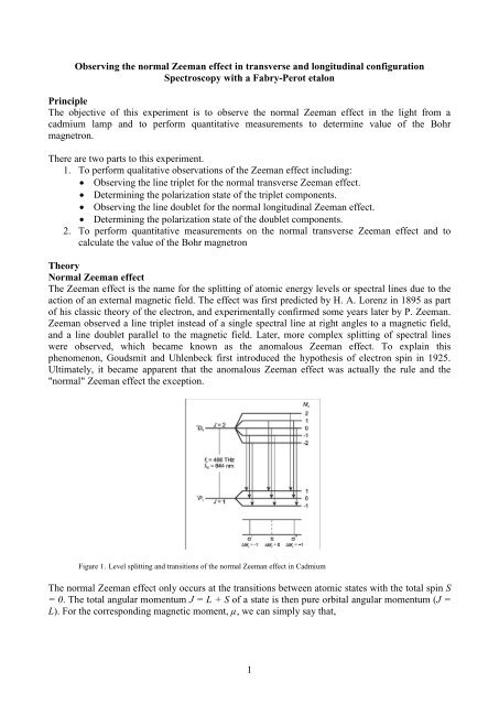
Figure 1. Level splitt<strong>in</strong>g <strong>and</strong> transitions of <strong>the</strong> <strong>normal</strong> <strong>Zeeman</strong> <strong>effect</strong> <strong>in</strong> Cadmium<br />
The <strong>normal</strong> <strong>Zeeman</strong> <strong>effect</strong> only occurs at <strong>the</strong> transitions between atomic states with <strong>the</strong> total sp<strong>in</strong> S<br />
= 0. The total angular momentum J = L + S of a state is <strong>the</strong>n pure orbital angular momentum (J =<br />
L). For <strong>the</strong> correspond<strong>in</strong>g magnetic moment, µ, we can simply say that,<br />
1
µ B µ = J<br />
(1)<br />
<br />
where<br />
e<br />
B =<br />
− 2m<br />
<br />
µ (2)<br />
e<br />
(μB = Bohr magnetron, me = mass of electron, e = elementary charge, = h/2π, h = Planck's<br />
constant).<br />
In an external magnetic field, B, <strong>the</strong> magnetic moment has <strong>the</strong> energy<br />
E = −µ<br />
B<br />
(3)<br />
The angular-momentum component <strong>in</strong> <strong>the</strong> direction of <strong>the</strong> magnetic field can have <strong>the</strong> values<br />
J z J<br />
J<br />
= M with M = J , J −1,....,<br />
−J<br />
(4)<br />
Therefore, <strong>the</strong> term with <strong>the</strong> angular momentum, J is split <strong>in</strong>to 2J + 1 equidistant <strong>Zeeman</strong><br />
components which differ by <strong>the</strong> value of MJ. The energy <strong>in</strong>terval of <strong>the</strong> adjacent components MJ,<br />
MJ+1 is<br />
∆ = µ B<br />
(5)<br />
E B<br />
We can observe <strong>the</strong> <strong>normal</strong> <strong>Zeeman</strong> <strong>effect</strong> e.g. <strong>in</strong> <strong>the</strong> red spectral l<strong>in</strong>e of cadmium (λ0 = 643.8 nm,<br />
f0 = 465.7 THz). It corresponds to <strong>the</strong> transition 1 D2 (J = 2, S = 0) → 1 P1 (J = 1, S = 0) of an<br />
electron of <strong>the</strong> fifth shell (see fig. 1). In <strong>the</strong> magnetic field, <strong>the</strong> 1 D2 level splits <strong>in</strong>to five <strong>Zeeman</strong><br />
components, <strong>and</strong> <strong>the</strong> level 1 P1 splits <strong>in</strong>to three <strong>Zeeman</strong> components hav<strong>in</strong>g <strong>the</strong> spac<strong>in</strong>g calculated<br />
us<strong>in</strong>g equation 5.<br />
Optical transitions between <strong>the</strong>se levels are only possible <strong>in</strong> <strong>the</strong> form of electrical dipole radiation.<br />
The follow<strong>in</strong>g selection rules apply for <strong>the</strong> magnetic quantum numbers MJ of <strong>the</strong> states <strong>in</strong>volved:<br />
∆<br />
M J<br />
⎧=<br />
± 1<br />
⎨<br />
⎩=<br />
0<br />
for σ components<br />
for π components<br />
Thus, we observe a total of three spectral l<strong>in</strong>es (see fig. 1); <strong>the</strong> π component is not shifted <strong>and</strong> <strong>the</strong><br />
two σ components are shifted by<br />
∆E<br />
∆ f = ±<br />
(7)<br />
h<br />
with respect to <strong>the</strong> orig<strong>in</strong>al frequency. In this equation, ΔE is <strong>the</strong> equidistant energy split calculated<br />
<strong>in</strong> equation 5.<br />
2<br />
(6)
Angular distribution <strong>and</strong> polarization<br />
Depend<strong>in</strong>g on <strong>the</strong> angular momentum component, ΔMJ, <strong>in</strong> <strong>the</strong> direction of <strong>the</strong> magnetic field, <strong>the</strong><br />
emitted photons exhibit different angular distributions. Figure 2 shows <strong>the</strong> angular distributions <strong>in</strong><br />
<strong>the</strong> form of two-dimensional polar diagrams. They can be observed experimentally, as <strong>the</strong> magnetic<br />
field is characterized by a common axis for all cadmium atoms.<br />
In classical terms, <strong>the</strong> case ΔMJ = 0 corresponds to an <strong>in</strong>f<strong>in</strong>itesimal dipole oscillat<strong>in</strong>g parallel to<br />
<strong>the</strong> magnetic field. No photons are emitted <strong>in</strong> <strong>the</strong> direction of <strong>the</strong> magnetic field, i.e. <strong>the</strong> πcomponent<br />
cannot be observed parallel to <strong>the</strong> magnetic field. The light emitted perpendicular to <strong>the</strong><br />
magnetic field is l<strong>in</strong>early polarized, whereby <strong>the</strong> E-vector oscillates <strong>in</strong> <strong>the</strong> direction of <strong>the</strong> dipole<br />
<strong>and</strong> parallel to <strong>the</strong> magnetic field (see fig. 3)<br />
Conversely, <strong>in</strong> <strong>the</strong> case ΔMJ = ±1 photons can be emitted both parallel <strong>and</strong> <strong>normal</strong> to <strong>the</strong> direction<br />
of <strong>the</strong> magnetic field. In classical terms, this case corresponds to two dipoles oscillat<strong>in</strong>g parallel to<br />
<strong>the</strong> magnetic field with a phase difference of 90°. The superposition of <strong>the</strong> two dipoles produces a<br />
circulat<strong>in</strong>g current. Thus, <strong>in</strong> <strong>the</strong> direction of <strong>the</strong> magnetic field, circularly polarized light is emitted;<br />
<strong>in</strong> <strong>the</strong> positive direction, it is clockwise-circular for ΔMJ = +1 <strong>and</strong> anticlockwise-circular for ΔMJ<br />
= -1 (see fig. 3).<br />
Figure 2. Angular distributions of <strong>the</strong> electrical dipole radiation (ΔM J: angular-momentum components of <strong>the</strong> emitted<br />
photons <strong>in</strong> <strong>the</strong> direction of <strong>the</strong> magnetic field)<br />
−<br />
σ<br />
( ∆M<br />
= −1)<br />
J<br />
π ( ∆M J =<br />
Figure 3. Schematic representation of <strong>the</strong> polarization of <strong>the</strong> <strong>Zeeman</strong> components (ΔM J:angular-momentum components of<br />
<strong>the</strong> emitted photons <strong>in</strong> <strong>the</strong> direction of <strong>the</strong> magnetic field)<br />
Spectroscopy of <strong>the</strong> <strong>Zeeman</strong> components<br />
The <strong>Zeeman</strong> <strong>effect</strong> enables spectroscopic separation of <strong>the</strong> differently polarized components.<br />
However, to demonstrate <strong>the</strong> shift we require an apparatus with extremely high spectral resolution,<br />
as <strong>the</strong> frequency of <strong>the</strong> two σ components of <strong>the</strong> red cadmium l<strong>in</strong>e are shifted, at a magnetic flux<br />
density B = 1T, by only 14GHz which is equivalent to a change <strong>in</strong> wavelength of only 0.02nm.<br />
3<br />
0)<br />
+<br />
σ ( ∆M<br />
= + 1)<br />
J
Figure 4. Fabry-Perot etalon as an <strong>in</strong>terference spectrometer. The ray path is drawn for an angle α > 0 relative to <strong>the</strong><br />
optical axis. The optical path difference between two adjacent emerg<strong>in</strong>g rays is Δ = n(Δ 1 – Δ 2)<br />
In this experiment a Fabry-Perot etalon is used to observe <strong>the</strong>se small changes <strong>in</strong> wavelength. A<br />
Fabry-Perot etalon is a glass plate where <strong>the</strong> two sides are parallel to a very high precision <strong>and</strong> with<br />
both sides alum<strong>in</strong>ized to make <strong>the</strong>m partially reflective. The slightly divergent light enters <strong>the</strong><br />
etalon, which is aligned perpendicularly to <strong>the</strong> optical axis, <strong>and</strong> is reflected back <strong>and</strong> forth several<br />
times, whereby part of it emerges each time (see Fig. 4). Due to <strong>the</strong> alum<strong>in</strong>iz<strong>in</strong>g this emerg<strong>in</strong>g part<br />
is small, i.e., many emerg<strong>in</strong>g rays can <strong>in</strong>terfere. Beh<strong>in</strong>d <strong>the</strong> etalon <strong>the</strong> emerg<strong>in</strong>g rays are focused by<br />
a lens <strong>and</strong> a concentric circular fr<strong>in</strong>ge pattern associated with a particular wavelength λ can be<br />
observed with an ocular (eye-piece).<br />
The rays emerg<strong>in</strong>g at an angle of αk <strong>in</strong>terfere constructively with each o<strong>the</strong>r when <strong>the</strong> path<br />
difference between <strong>the</strong> rays is equal to a whole number of wavelengths (see Fig. 4)<br />
∆ = ∆<br />
1<br />
∆ −<br />
2<br />
d n α k kλ<br />
= − =<br />
2 2<br />
2 s<strong>in</strong><br />
(8)<br />
Δ = optical path difference, d = thickness of <strong>the</strong> etalon, n = refractive <strong>in</strong>dex of <strong>the</strong> glass, k = order<br />
of <strong>in</strong>terference.<br />
A change <strong>in</strong> <strong>the</strong> wavelength of δλ is seen as a change <strong>in</strong> <strong>the</strong> angle, α, of <strong>the</strong> emerg<strong>in</strong>g ray of δα.<br />
Depend<strong>in</strong>g on <strong>the</strong> focal length of <strong>the</strong> lens, <strong>the</strong> angle, α, corresponds to a radius, r, <strong>and</strong> <strong>the</strong> change <strong>in</strong><br />
<strong>the</strong> angle δα to a change <strong>in</strong> <strong>the</strong> radius δr. If a spectral l<strong>in</strong>e conta<strong>in</strong>s several components with a<br />
difference <strong>in</strong> wavelength of δλ, each circular <strong>in</strong>terference fr<strong>in</strong>ge is split <strong>in</strong>to as many components<br />
with <strong>the</strong> radial distance δr. So a spectral l<strong>in</strong>e doublet is recognized by a doublet structure <strong>and</strong> a<br />
spectral l<strong>in</strong>e triplet by a triplet structure <strong>in</strong> <strong>the</strong> circular fr<strong>in</strong>ge pattern.<br />
Part 1. Qualitative observation of <strong>the</strong> <strong>normal</strong> <strong>Zeeman</strong> <strong>effect</strong><br />
Setup<br />
The complete experimental setup <strong>in</strong> <strong>transverse</strong> configuration is illustrated <strong>in</strong> Fig. 5.<br />
4
Cd<br />
lamp<br />
Condenser<br />
lens<br />
Polariser<br />
Figure 5. Experimental setup for observ<strong>in</strong>g <strong>the</strong> <strong>Zeeman</strong> <strong>effect</strong> <strong>in</strong> <strong>transverse</strong> configuration. The position of <strong>the</strong> left edge of<br />
<strong>the</strong> optics riders is given <strong>in</strong> cm.<br />
Mechanical <strong>and</strong> optical setup:<br />
• The cadmium lamp <strong>and</strong> magnet should be mounted on <strong>the</strong> rail when you arrive. Be very<br />
careful with mov<strong>in</strong>g <strong>the</strong> magnet assembly as <strong>the</strong> cadmium lamp is very fragile (<strong>and</strong><br />
expensive!)<br />
• Mount <strong>the</strong> optical components accord<strong>in</strong>g to Fig. 5.<br />
Electrical connection:<br />
• Connect <strong>the</strong> cadmium lamp to <strong>the</strong> power supply; after switch<strong>in</strong>g on wait 5 m<strong>in</strong> until <strong>the</strong><br />
light emission is bright blue.<br />
• Connect <strong>the</strong> coils of <strong>the</strong> electromagnet <strong>in</strong> series <strong>and</strong> <strong>the</strong>n to <strong>the</strong> high current power supply.<br />
• The Hall probe for measur<strong>in</strong>g <strong>the</strong> magnetic field must NEVER be placed <strong>in</strong> <strong>the</strong> magnet<br />
when <strong>the</strong> lamp is on.<br />
• Only <strong>in</strong>crease <strong>the</strong> current flow<strong>in</strong>g through <strong>the</strong> magnet when it is be<strong>in</strong>g used. The magnet<br />
rapidly heats up when <strong>in</strong> use so always turn <strong>the</strong> current back to zero when not observ<strong>in</strong>g <strong>the</strong><br />
fr<strong>in</strong>ge pattern.<br />
Adjust<strong>in</strong>g <strong>the</strong> observ<strong>in</strong>g optics:<br />
The optimum setup is achieved when <strong>the</strong> red circular fr<strong>in</strong>ge pattern is bright with strong contrast<br />
<strong>and</strong> centred on <strong>the</strong> l<strong>in</strong>e graduation. While adjust<strong>in</strong>g remove <strong>the</strong> polarization filter so that <strong>the</strong><br />
observed image is as bright as possible.<br />
• Focus <strong>the</strong> ocular at <strong>the</strong> l<strong>in</strong>e graduation.<br />
• Move <strong>the</strong> imag<strong>in</strong>g lens until you observe a sharply def<strong>in</strong>ed image of <strong>the</strong> circular fr<strong>in</strong>ge<br />
pattern.<br />
• Move <strong>the</strong> condenser lens until <strong>the</strong> observed image is illum<strong>in</strong>ated as uniformly as possible.<br />
• Shift <strong>the</strong> centre of <strong>the</strong> circular fr<strong>in</strong>ge pattern to <strong>the</strong> middle of <strong>the</strong> l<strong>in</strong>e graduation by slightly<br />
tipp<strong>in</strong>g <strong>the</strong> Fabry-Perot etalon with <strong>the</strong> adjust<strong>in</strong>g screws.<br />
If <strong>the</strong> adjustment range does is not sufficient <strong>the</strong>n gently rotate <strong>the</strong> Fabry-Perot etalon with its<br />
frame or adjust <strong>the</strong> height of <strong>the</strong> imag<strong>in</strong>g lens <strong>and</strong> <strong>the</strong> ocular relative to each o<strong>the</strong>r.<br />
Carry<strong>in</strong>g out <strong>the</strong> experiment<br />
a) <strong>Observ<strong>in</strong>g</strong> <strong>in</strong> <strong>transverse</strong> configuration:<br />
• First observe <strong>the</strong> circular fr<strong>in</strong>ge pattern without magnetic field (I = 0 A).<br />
• Slowly enhance <strong>the</strong> magnet current until <strong>the</strong> fr<strong>in</strong>ges split <strong>and</strong> are clearly separated.<br />
• Record what you observe.<br />
To dist<strong>in</strong>guish between π <strong>and</strong> σ components:<br />
• Introduce <strong>the</strong> polarization filter <strong>in</strong>to <strong>the</strong> ray path (see Fig. 5) <strong>and</strong> set it to 90° where <strong>the</strong> two<br />
outer components of <strong>the</strong> triplet structure should disappear.<br />
5<br />
Etalon<br />
Imag<strong>in</strong>g lens<br />
f=150 mm f=150 mm<br />
Interference<br />
filter<br />
Eyepiece<br />
λ=643.8 nm
• Set <strong>the</strong> polarization filter to 0° <strong>and</strong> <strong>the</strong> (unshifted) component <strong>in</strong> <strong>the</strong> middle should<br />
disappear.<br />
b) <strong>Observ<strong>in</strong>g</strong> <strong>in</strong> longitud<strong>in</strong>al configuration:<br />
• Carefully rotate <strong>the</strong> entire setup of <strong>the</strong> cadmium lamp with <strong>the</strong> magnet by 90°.<br />
• First observe <strong>the</strong> circular fr<strong>in</strong>ge pattern without magnetic field (I = 0 A).<br />
• Slowly <strong>in</strong>crease <strong>the</strong> magnet current until <strong>the</strong> split fr<strong>in</strong>ges <strong>and</strong> are clearly separated.<br />
• Record what you observe.<br />
To dist<strong>in</strong>guish between σ + <strong>and</strong> σ - components:<br />
• Introduce a quarter-wavelength plate <strong>in</strong>to <strong>the</strong> ray path between <strong>the</strong> cadmium lamp <strong>and</strong> <strong>the</strong><br />
polarization filter <strong>and</strong> set it to 0°.<br />
• Set <strong>the</strong> polarization filter to +45° <strong>and</strong> –45°. In each case one of <strong>the</strong> two doublet components<br />
should disappear.<br />
Part 2. Quantitative measurements of <strong>the</strong> <strong>Zeeman</strong> <strong>effect</strong><br />
To perform quantitative measurements of <strong>the</strong> splitt<strong>in</strong>g of <strong>the</strong> red cadmium spectral l<strong>in</strong>e as a<br />
function of magnetic flux density <strong>the</strong> eyepiece, used for <strong>the</strong> first part of <strong>the</strong> experiment, is replaced<br />
with <strong>the</strong> l<strong>in</strong>ear CCD array <strong>and</strong> <strong>the</strong> <strong>in</strong>tensity of a l<strong>in</strong>e through <strong>the</strong> r<strong>in</strong>g system of <strong>the</strong> <strong>in</strong>terferometer is<br />
displayed on <strong>the</strong> PC. To perform quantitative measurements <strong>the</strong> lamp is place <strong>in</strong> <strong>the</strong> <strong>transverse</strong><br />
configuration. The basic configuration should look like <strong>the</strong> schematic diagram shown <strong>in</strong> figure 6.<br />
Make sure <strong>the</strong> <strong>in</strong>terference filter is as close as possible to <strong>the</strong> CCD array so as to stop room light<br />
hitt<strong>in</strong>g <strong>the</strong> array.<br />
Cd<br />
lamp<br />
Condenser<br />
lens<br />
Polariser<br />
Figure 6. Schematic diagram of optical setup for quantitative measurements<br />
Adjust<strong>in</strong>g <strong>the</strong> setup<br />
The software for <strong>the</strong> CCD camera can be used to adjust <strong>the</strong> camera sett<strong>in</strong>gs to optimise data<br />
collection. For <strong>the</strong> <strong>in</strong>itial sett<strong>in</strong>g up of <strong>the</strong> experiment set <strong>the</strong> camera to use only 256 pixels (button<br />
with a camera <strong>and</strong> I <strong>in</strong> <strong>the</strong> corner). This will allow <strong>the</strong> screen to be refreshed more quickly which<br />
aids <strong>in</strong> sett<strong>in</strong>g up <strong>the</strong> experiment. Once <strong>the</strong> setup is complete set <strong>the</strong> camera to 2048 pixels (button<br />
with a camera <strong>and</strong> II <strong>in</strong> <strong>the</strong> corner). It is also possible to adjust <strong>the</strong> exposure time (us<strong>in</strong>g <strong>the</strong> buttons<br />
with a magnify<strong>in</strong>g glass) so that <strong>the</strong> peaks have an <strong>in</strong>tensity of approximately 50 %.<br />
To ensure that <strong>the</strong> CCD is <strong>in</strong> <strong>the</strong> focal plane of <strong>the</strong> imag<strong>in</strong>g lens (f = 150 mm), move <strong>the</strong> imag<strong>in</strong>g<br />
lens along <strong>the</strong> optical axis until <strong>the</strong> peaks of <strong>the</strong> observed curve are sharply imaged <strong>and</strong> show <strong>the</strong><br />
maximum <strong>in</strong>tensity. The centre of <strong>the</strong> r<strong>in</strong>g system must <strong>the</strong>n be imaged on <strong>the</strong> CCD l<strong>in</strong>e. For this,<br />
you can ei<strong>the</strong>r move <strong>the</strong> VideoCom perpendicular to <strong>the</strong> optical axis or tilt <strong>the</strong> etalon <strong>in</strong>terferometer<br />
slightly us<strong>in</strong>g <strong>the</strong> adjust<strong>in</strong>g screws. The centre of <strong>the</strong> r<strong>in</strong>g system is on <strong>the</strong> CCD l<strong>in</strong>e when fur<strong>the</strong>r<br />
adjustment does not cause any more peaks to emerge <strong>and</strong> <strong>the</strong> two central peaks (left <strong>and</strong> right<br />
<strong>in</strong>tersections of <strong>the</strong> <strong>in</strong>nermost r<strong>in</strong>gs) are <strong>the</strong> maximum distance apart.<br />
Move <strong>the</strong> condenser lens until you obta<strong>in</strong> uniform illum<strong>in</strong>ation of <strong>the</strong> entire CCD l<strong>in</strong>e.<br />
6<br />
Etalon<br />
Imag<strong>in</strong>g lens<br />
f=150 mm f=150 mm<br />
Interference<br />
filter<br />
λ=643.8 nm
Diffraction Angle Calibration<br />
Before you can determ<strong>in</strong>e <strong>the</strong> change <strong>in</strong> <strong>the</strong> wavelength of <strong>the</strong> l<strong>in</strong>es, <strong>the</strong> <strong>in</strong>dividual pixels of <strong>the</strong><br />
CCD must be calibrated to diffraction angle, α. For an imag<strong>in</strong>g lens of <strong>effect</strong>ive focal length, f , <strong>the</strong><br />
diffraction angle can be calculated us<strong>in</strong>g α=arctan(x/f) where x=(1024-p)*14µm where p = pixel<br />
coord<strong>in</strong>ate on <strong>the</strong> CCD (0 to 2047). This is performed automatically <strong>in</strong> <strong>the</strong> software by enter<strong>in</strong>g <strong>the</strong><br />
value for <strong>the</strong> focal length of <strong>the</strong> imag<strong>in</strong>g lens used (f=150mm) <strong>in</strong>to <strong>the</strong> set up screen. Ask <strong>the</strong><br />
demonstrators for help with this part of <strong>the</strong> software if necessary. This calibration changes <strong>the</strong><br />
horizontal axis to degrees.<br />
It is now necessary to set <strong>the</strong> zero position to <strong>the</strong> centre of <strong>the</strong> r<strong>in</strong>g pattern. Use <strong>the</strong> zoom <strong>and</strong><br />
display coord<strong>in</strong>ates functions to determ<strong>in</strong>e <strong>the</strong> angles of <strong>the</strong> two central peaks <strong>and</strong> use <strong>the</strong> mean of<br />
<strong>the</strong>se as <strong>the</strong> zero po<strong>in</strong>t shift. Enter <strong>the</strong> negative value of this <strong>in</strong>to <strong>the</strong> “shift zero po<strong>in</strong>t” box. This<br />
should set <strong>the</strong> centre of <strong>the</strong> r<strong>in</strong>g system to 0° on <strong>the</strong> angular scale.<br />
Quantitative evaluation<br />
The aim of this part of <strong>the</strong> experiment is to measure how much <strong>the</strong> peaks shift with an applied<br />
magnetic field. The angle of <strong>the</strong> peak without an applied field is α0 <strong>and</strong> you can record a series of<br />
values of <strong>the</strong> peak position with <strong>in</strong>creas<strong>in</strong>g magnetic field, α1.<br />
The <strong>in</strong>tensity of <strong>the</strong> peaks should be around 50 % (adjust this if necessary as <strong>the</strong> lum<strong>in</strong>ance of <strong>the</strong><br />
Cd lamp changes <strong>in</strong> <strong>the</strong> magnetic field). Use <strong>the</strong> zoom <strong>and</strong> display coord<strong>in</strong>ates function to<br />
determ<strong>in</strong>e <strong>the</strong> centre of one of <strong>the</strong> peaks with <strong>the</strong> magnetic flux density at 0T (α0). Record <strong>the</strong><br />
position of one of <strong>the</strong> peaks (α1) as <strong>the</strong> magnet current is <strong>in</strong>creased (use steps of 0.5A <strong>in</strong> <strong>the</strong> current<br />
through <strong>the</strong> magnet). The value of <strong>the</strong> magnetic flux density can be found for each value of magnet<br />
current at <strong>the</strong> end of <strong>the</strong> experiment. When you have f<strong>in</strong>ished all <strong>the</strong> measurements <strong>and</strong> <strong>the</strong> lamp is<br />
switched off place <strong>the</strong> Hall probe carefully <strong>in</strong>to <strong>the</strong> centre of <strong>the</strong> magnet (It is <strong>the</strong> small square<br />
which is <strong>the</strong> sensor <strong>and</strong> this should be visible through <strong>the</strong> hole <strong>in</strong> <strong>the</strong> magnet pole pieces). Then<br />
record <strong>the</strong> magnetic flux density as a function of magnet current.<br />
Repeat <strong>the</strong> measurements <strong>in</strong> <strong>the</strong> longitud<strong>in</strong>al configuration us<strong>in</strong>g <strong>the</strong> quarter-wave plate <strong>and</strong><br />
polariser.<br />
You should now have two tables of angular position of <strong>the</strong> peak, α1, as a function of magnetic flux<br />
density, B. The aim is to convert this <strong>in</strong>to a shift <strong>in</strong> <strong>the</strong> energy of <strong>the</strong> peak so that equation 5 can be<br />
used to measure <strong>the</strong> value of <strong>the</strong> Bohr magnetron, μB. If one knew <strong>the</strong> <strong>in</strong>terference order, k, for <strong>the</strong><br />
peak you are measur<strong>in</strong>g <strong>the</strong>n know<strong>in</strong>g <strong>the</strong> angular position of <strong>the</strong> peak <strong>and</strong> <strong>the</strong> thickness <strong>and</strong><br />
refractive <strong>in</strong>dex of <strong>the</strong> etalon, one would be able to determ<strong>in</strong>e <strong>the</strong> wavelength of <strong>the</strong> peak from<br />
equation 8. Unfortunately, it is not possible to know <strong>the</strong> <strong>in</strong>terference order for any particular peak.<br />
However, each peak has a s<strong>in</strong>gle value of k <strong>and</strong> as <strong>the</strong> peak moves with magnetic flux density this<br />
is due to <strong>the</strong> change <strong>in</strong> wavelength with k rema<strong>in</strong><strong>in</strong>g constant. It is <strong>the</strong>refore possible to determ<strong>in</strong>e<br />
<strong>the</strong> relative shift <strong>in</strong> wavelength, Δλ/λ, from <strong>the</strong> shift <strong>in</strong> <strong>the</strong> angular position of a given peak.<br />
If <strong>the</strong> angular position of <strong>the</strong> peak at zero magnetic field is α0, <strong>the</strong>n <strong>the</strong> relative shift <strong>in</strong> wavelength<br />
is given by,<br />
∆λ<br />
cos β<br />
=<br />
λ cos β<br />
where<br />
1 −<br />
0<br />
1<br />
s<strong>in</strong>α<br />
n = 1 . 46 =<br />
(10)<br />
s<strong>in</strong> β<br />
7<br />
(9)
where α is <strong>the</strong> external angle a ray makes with <strong>the</strong> etalon (what you are measur<strong>in</strong>g) <strong>and</strong> β is <strong>the</strong><br />
<strong>in</strong>ternal angle <strong>the</strong> same ray makes <strong>in</strong>side <strong>the</strong> etalon. Equation 9 is derived from equation 8, <strong>and</strong><br />
equation 10 is Snell’s Law.<br />
Us<strong>in</strong>g <strong>the</strong>se equations calculate Δλ/λ as a function of magnetic flux density for your data. F<strong>in</strong>ally<br />
you need to convert Δλ/λ to ΔE. To do this use equation 11.<br />
∆λ<br />
∆λ<br />
∆E = − E = −hc<br />
(11)<br />
2<br />
λ λ<br />
where λ=643.8 nm for <strong>the</strong> cadmium l<strong>in</strong>e. Use your data to calculate <strong>the</strong> value of <strong>the</strong> Bohr<br />
magnetron, μB.<br />
The literature value is 57.9 μeV/T.<br />
Derivation of equation 9<br />
Any given peak has a value of k <strong>and</strong> as λ changes due to <strong>the</strong> magnetic field k rema<strong>in</strong>s constant,<br />
Therefore,<br />
∆λ<br />
2<br />
=<br />
λ<br />
∆λ<br />
=<br />
λ<br />
2 2<br />
2<br />
d n − s<strong>in</strong> α1<br />
− 2d<br />
n −<br />
⎛ n<br />
⎜<br />
⎝ n<br />
From Snell’s law<br />
2<br />
2<br />
2d<br />
n<br />
2<br />
s<strong>in</strong><br />
2<br />
− s<strong>in</strong> α ⎞ 1<br />
−1<br />
2<br />
s<strong>in</strong> ⎟<br />
− α 0 ⎠<br />
2<br />
α<br />
0<br />
s<strong>in</strong><br />
2<br />
α<br />
0<br />
s<strong>in</strong>α = ns<strong>in</strong><br />
β<br />
(14)<br />
2 2 2<br />
2<br />
2 2<br />
n s<strong>in</strong> α = n ( 1−<br />
s<strong>in</strong> β ) = n cos β<br />
(15)<br />
∆λ<br />
=<br />
λ<br />
⎛ n<br />
⎜<br />
⎝ n<br />
2<br />
2<br />
cos<br />
cos<br />
2<br />
2<br />
β ⎞ 1 cos β1<br />
⎟ −1<br />
= −1<br />
β 0 ⎠ cos β 0<br />
8<br />
(12)<br />
(13)<br />
(16)