Improving crosshole radar velocity tomograms - Stanford Woods ...

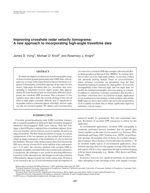
GEOPHYSICS, VOL. 72, NO. 4 JULY-AUGUST 2007; P. J31–J41, 12 FIGS.
10.1190/1.2742813
Improving crosshole radar velocity tomograms:
A new approach to incorporating high-angle traveltime data
James D. Irving 1 , Michael D. Knoll 2 , and Rosemary J. Knight 3
ABSTRACT
To obtain the highest-resolution ray-based tomographic images
from crosshole ground-penetrating radar GPR data, wide angular
ray coverage of the region between the two boreholes is required.
Unfortunately, at borehole spacings on the order of a few
meters, high-angle traveltime data i.e., traveltime data corresponding
to transmitter-receiver angles greater than approximately
50° from the horizontal are notoriously difficult to incorporate
into crosshole GPR inversions. This is because 1 low
signal-to-noise ratios make the accurate picking of first-arrival
times at high angles extremely difficult, and 2 significant tomographic
artifacts commonly appear when high- and low-angle
ray data are inverted together. We address and overcome these
INTRODUCTION
Crosshole ground-penetrating radar GPR traveltime tomography
is a popular geophysical method for high-resolution imaging of
subsurface electromagnetic EM wave velocity. With this technique,
a short EM pulse is radiated from a transmitter antenna, located
in one borehole, and recorded at a receiver antenna, located in an
adjacent borehole. The first-break traveltimes of energy for various
configurations of the two antennas are then picked and inverted to
obtain an image tomogram of the distribution of velocity between
the boreholes. Because of the strong contrast that exists between the
EM-wave velocity of water 0.03 m/ns and that of dry earth materials
0.15 m/ns, the velocities obtained with crosshole GPR tomography
are highly correlated with water content in the subsurface.
Consequently, the technique is very useful for detecting differences
in porosity in the saturated zone, and changes in soil water retention
often linked to changes in grain size in the vadose zone. Of interest
in our research is the use of such information in the development of
two issues for a crosshole GPR data example collected at the Boise
Hydrogeophysical Research Site BHRS. To estimate firstarrival
times on noisy, high-angle gathers, we develop a robust
and automatic picking strategy based on crosscorrelations,
where reference waveforms are determined from the data
through the stacking of common-ray-angle gathers. To overcome
incompatibility issues between high- and low-angle data, we
modify the standard tomographic inversion strategy to estimate,
in addition to subsurface velocities, parameters that describe a
traveltime ‘correction curve’ as a function of angle. Application
of our modified inversion strategy, to both synthetic data and the
BHRS data set, shows that it allows the successful incorporation
of all available traveltime data to obtain significantly improved
subsurface velocity images.
numerical models for groundwater flow and contaminant transport.
Resolution of crosshole GPR tomograms is critical for this
application.
In environmental applications, crosshole GPR tomography is
commonly performed between boreholes that are spaced quite
closely together on the order of a few meterse.g., Peterson, 2001;
Alumbaugh and Chang, 2002; Tronicke et al., 2002b. At such borehole
spacings, the potential exists in theory for excellent tomographic
resolution. This is because, even for the relatively shallow 20
m borehole depths typical of environmental applications, close
borehole spacings allow for wide angular coverage of the inter-borehole
region, which is a key requirement for high-resolution imaging
with ray-based tomography e.g., Menke, 1984; Rector and Washbourne,
1994.
In practice, however, two significant problems are encountered
when attempting to take advantage of this wide angular coverage.
Manuscript received by the Editor February 1, 2007; published online June 20, 2007.
1 Formerly Stanford University, Department of Geophysics, Stanford, California; presently University of Lausanne, Institute of Geophysics, Lausanne, Switzerland.
E-mail: james.d.irving@gmail.com.
2 Formerly Boise State University, Department of Geosciences, Boise, Idaho; presently Boise, Idaho. E-mail: miknoll@gmail.com.
3 Stanford University, Department of Geophysics, Stanford, California. E-mail: rknight@pangea.stanford.edu.
© 2007 Society of Exploration Geophysicists.All rights reserved.
J31

J32 Irving et al.
First, the arrival times of energy traveling at high transmitter-receiver
angles commonly, angles greater than 50° from the horizontal
are often very difficult to pick because of low signal-to-noise ratios
S/N in the data. This results not only because of an increased
amount of attenuation at high angles arising from longer travel
paths, but also because of the radiation patterns of the crosshole GPR
antennas, which decrease to zero amplitude along the end-fire directions
e.g., Peterson, 2001; Holliger and Bergmann, 2002. Second,
even when high-angle traveltimes can be determined reliably at
close borehole spacings, difficulties are commonly encountered
when attempting to incorporate these data into crosshole GPR inversions.
Specifically, the high-angle data often appear to be incompatible
with the lower-angle data available, and cause significant numerical
artifacts in the resulting tomograms Peterson, 2001; Alumbaugh
and Chang, 2002; Irving and Knight, 2005a. As a result, current
practice is to exclude high-angle traveltime data from crosshole
GPR inversions e.g., Alumbaugh and Chang, 2002; Linde et al.,
2006. This has the advantage of allowing reasonable subsurface images
to be obtained. However, it comes at the cost of reduced horizontal
resolution; high-angle data are necessary to constrain the lateral
variability of the subsurface velocity field. Depending on the
end use of the crosshole GPR images, this reduction in horizontal
resolution may be a serious drawback.
In this paper, we present a case study attempting to address rather
than avoid the above two issues for a crosshole GPR data set collected
at the Boise Hydrogeophysical Research Site BHRS. To
overcome the high-angle picking problem, we develop a strategy for
determining first-break times from crosshole GPR data using crosscorrelations.
With this technique, picking of the example data set is
accomplished automatically and reliably, even for traces with very
low S/N corresponding to high transmitter/receiver angles. To address
the high-angle incompatibility problem at close borehole spacings,
we first discuss what we believe to be the cause of this problem
for the BHRS data set. Using this information, we then develop a
modified inversion strategy that allows all available traveltimes
both high- and low-angle to be incorporated successfully into the
tomographic reconstruction.
FIELD SITE AND DATA DESCRIPTION
The BHRS is a research wellfield located near Boise, Idaho in a
shallow, unconfined aquifer Barrash et al., 1999. The aquifer consists
of an approximately 18-m-thick layer of coarse, unconsolidated,
braided-stream deposits gravels and cobbles with sand lenses,
and is underlain by clay and basalt. The purpose of developing the
BHRS was to create a site for testing geophysical and hydrologic
methods, with the goal of using these methods to characterize the
distribution of hydrogeological properties in heterogeneous alluvial
aquifers. Eighteen wells have been emplaced at the site, all of which
were carefully completed to minimize disturbance of the surrounding
formation and cased with 4-in PVC well screen Barrash and
Knoll, 1998. For additional information about the BHRS, including
the different stratigraphic units that have been identified using welllog,
core, and geophysical data, see Barrash and Clemo 2002, Barrash
and Reboulet 2004, Tronicke et al. 2004, Clement et al.
2006, Clement and Barrash 2006, and Moret et al. 2006.
The crosshole GPR field data analyzed in this study were collected
at the BHRS between wells labeledA1 and B2 during the summer
of 1999. These two wells are approximately 3.5 m apart and 20 m
deep. The Malå RAMAC/GPR borehole antennas used for the cross-
hole survey had a specified center frequency of 250 MHz. To conduct
the survey, common-receiver gathers were collected. The receiver
antenna, located in well B2, was lowered every 0.2 m. For
each receiver location, the transmitter antenna located in well A1
was fired approximately every 0.05 m as it was lowered down the
borehole. The resulting crosshole GPR data set contained over
25,000 traces. Because much of this information is redundant and
not necessary to obtain the highest-possible-resolution ray-based tomographic
image, we considered data from every fourth transmitter
location in our analysis. Subsampling in this manner made the
depth-sampling intervals in the transmitter and receiver boreholes
approximately equal. In addition, we considered only those traces
where both the transmitter and receiver antenna elements were contained
entirely below the water table determined using a water level
meter to be at approximately 3 m depth at the time of the survey.
The final data set analyzed, representative of the saturated zone between
3.6 and 18.2 m depth, contained 5329 traces with transmitter/
receiver angles ranging from 75° to 75° from the horizontal.
To account for borehole deviations in our analysis — a critical
step in crosshole GPR tomography, especially at close borehole
spacings Peterson, 2001 — borehole trajectories in the subsurface
were measured carefully using a magnetic deviation logging tool. To
minimize deviations of the transmitter and receiver locations from
the tomographic plane, we applied a very slight coordinate rotation
to the data such that, in the new coordinate system, all borehole deviations
were constrained to within 3 cm of this plane. Parameters for
the rotation were determined using an inversion that minimized the
sum of the squared out-of-plane deviations. Finally, the GPR system
sampling frequency and transmitter fire time were determined carefully
before the survey by firing the antennas in air in a walkaway
survey using a calibrated survey tape.
CROSSCORRELATION PICKING
OF TRAVELTIMES
Figure 1 shows an example common-receiver gather from the
BHRS data set, corresponding to a receiver depth of 5.33 m.All traces
in the gather have been normalized by their maximum amplitudes
for easier comparison. The figure clearly illustrates why difficulties
are often encountered when attempting to pick first breaks in highangle
crosshole GPR data. Notice that when the antenna depths are
similar near the top of the plot, the recorded waveforms have a very
strong S/N and picking of first breaks is straightforward; on the uppermost
trace, the first break occurs just before the small positive
peak located at approximately 55 ns. However, as the transmitter
depth and thus the angle between antennas increases, the S/N decreases
to the point where, near the bottom of Figure 1, the first-arriving
peak cannot even be seen, let alone picked.Although low-pass
filtering may be of some help in attempting to pick such noisy traces,
the large amount of filtering required for traces with very low S/N often
can affect significantly the apparent onset of signal.Another idea
might be to pick the point of maximum amplitude on the noisy traces
and then back off a prescribed amount to obtain the first breaks.
However, such picking is not robust. More importantly, the position
of the first break with respect to the trace maximum will vary with
transmitter/receiver angle because the GPR waveform changes with
angle. Clearly, signal is present in the lower traces of Figure 1; its onset
is simply overshadowed by noise. The question is: Can we find a
way to use what signal is there to estimate the first arrivals?

One solution for the robust estimation of traveltimes in the presence
of significant noise, that has been used widely in earthquake
and exploration seismic studies, is the crosscorrelation technique
e.g., Peraldi and Clement, 1972; VanDecar and Crosson, 1990;
Woodward and Masters, 1991; Molyneux and Schmitt, 1999. With
this method, the discrete crosscorrelation of a trace and a high-quality
reference waveform having a known arrival time is determined,
and then the difference in traveltime between the two signals is obtained
from the time shift at which the crosscorrelation value is a
maximum.
Ideally, the reference waveform used with this technique should
be noise-free and have the same shape as the waveform present on
the trace in question. Although synthetics are often used to obtain
such a waveform in earthquake studies, we obtained reference waveforms
for crosscorrelation picking of the BHRS data set from the
data themselves. We found that synthetic modeling required too
much knowledge about GPR system, antenna, and earth parameters
to yield waveforms that were sufficiently close enough to those in
the field data for effective crosscorrelation analysis. To obtain the
reference waveforms, we stack traces that have been aligned on the
first arrival. Because the GPR pulse changes with transmitter/receiver
angle a result of variations in antenna radiation and reception
with angle, and likely also propagation dispersion along travel paths
having different lengths, we determine a number of different reference
waveforms that represent ranges in angle where the arriving
pulses have similar shape.
Figure 2 is a flowchart illustrating the sequence of steps involved
in our crosscorrelation picking procedure. The crosshole GPR data
are first preprocessed by removing any DC offset from each trace
determined from the mean value of the trace before the onset of signal
and by normalizing each trace by the signal maximum estimated
by low-pass filtering the data and finding the maximum value.If
desired, extremely noisy traces with no apparent signal can be discarded
straightaway to reduce the number of bad picks obtained with
the technique. Next, the crosshole data are sorted into common-rayangle
gathers e.g., Pratt and Worthington, 1988; Pratt and Goulty,
1991; Tronicke et al., 2002a. To do this, we create a set of angle bins
Transmitter depth (m)
4
6
8
10
12
14
16
18
40 60 80 100 120 140 160 180 200
Time (ns)
Figure 1. Common-receiver gather from the BHRS data set showing
the difficulties in picking first-break times at high transmitter-receiver
angles arising from low S/N. Receiver depth is 5.33 m. All traces
have been normalized by their maximum values.
Incorporating high-angle traveltime data J33
and place each trace into the appropriate bin based on the transmitter/receiver
angle. To determine a high-quality reference waveform
for each angle bin, the waveforms in each gather must be aligned and
then stacked.
Because aligning the traces requires some means of estimating the
relative time shifts between the waveforms, we use crosscorrelations,
but in an iterative manner as follows: Initially, the traces in a
common-ray-angle gather are aligned by crosscorrelating them with
the trace in the gather having the highest S/N. This places the majority
of traces into proper alignment, which allows for a higher quality
waveform to be obtained through stacking. In the second iteration,
traces in the gather are aligned again, but this time by crosscorrelating
them with the mean trace from the previous iteration. This process
can be continued until the vast majority of traces in a gather are
properly aligned; however, we have found that two iterations are
usually sufficient.
Once the reference waveforms for each angle range have been determined,
their first arrivals are picked manually. The entire crosshole
data set is then picked automatically by crosscorrelating each
trace with the appropriate reference waveform. To increase the robustness
of this algorithm, we limit the number of lags used in the
crosscorrelations to reasonable values i.e., for the BHRS data set,
absolute differences in arrival time between individual traces and the
reference trace were assumed to be less than 20 ns. As a final step,
all of the automatic picks made with this method should be checked
visually for accuracy. Bad picks are generally quite obvious, as they
Data preprocessing
1) remove DC shift from each trace
2) normalize each trace by signal maximum
3) discard data where signal is clearly absent
Sort data into common-ray-angle gathers
Align traces in each common-ray-angle
gather by crosscorrelating with either:
1) trace having highest signal-to-noise ratio
2) mean trace from previous iteration
Determine mean trace for each angle gather
Another iteration
needed to properly align traces
in each gather?
Pick first-arrival time on each mean trace
Crosscorrelate each trace in data set with
appropriate reference waveform for that angle,
and use to determine first-arrival time
Manually inspect the picks
Done
No
Yes
Figure 2. Flowchart of our crosscorrelation picking procedure.

J34 Irving et al.
tend to be caused by the crosscorrelation being maximized when the
two signals are mismatched by a full cycle.
As an example, Figure 3a shows one of the common-ray-angle
gathers obtained from the BHRS data set for the 65° to 70° angle
range. Here, the transmitter/receiver angle is measured from the horizontal
with positive angles representing the case where the receiver
antenna is located above the transmitter antenna. Two iterations of
crosscorrelating were used to align the traces in this high-angle gather.
The waveforms in the gather are clearly visible and have very
similar shapes, but they are contaminated by significant amounts of
noise which makes picking the first breaks extremely difficult. Figure
3b, on the other hand, shows the mean trace that was obtained by
stacking the 322 traces in Figure 3a together. Here, we see that the
S/N has been greatly increased and that a small, positive, first-arrival
peak, not clearly visible on any individual trace, is now easily identified.
The much higher S/N of this mean trace, and the fact that its first
break can be picked easily, make it an excellent reference waveform
for crosscorrelation analysis.
Figure 4 shows the mean traces that were obtained in the above
manner for each angle group in the BHRS data set. The waveforms
have been aligned on their manually picked first arrivals for easier
comparison. Angle bins were created for every 5° increment from
75° to 75°, which yielded 30 reference waveforms. Figure 4
clearly shows why we must determine these waveforms as a function
of angle when picking crosshole GPR data, as opposed to using a sin-
a) b)
Time (ns)
80
100
120
140
160
180
200
0 50 100 150 200 250 300
200
−1 0 1
Trace number
Amplitude
Figure 3. a Common-ray-angle gather and b mean trace for the
65° to 70° angle range in the BHRS data set. The picked first-arrival
time on the mean trace is indicated with a horizontal dashed line.
Time (ns)
0
20
40
60
80
100
120
140
160
180
80
80 −60 −40 −20 0 20 40 60 80
Angle bin center (°)
Figure 4. Mean traces determined for the BHRS data set by stacking
the different common-ray-angle gathers. The traces have been
aligned at t = 0 on their picked first arrivals and normalized by their
maximum values.
gle reference waveform for the entire data set; there is a significant
change in shape of the GPR pulse with angle that must be accounted
for. Also notice that all of the reference waveforms in Figure 4, including
the ones on both ends if scaled enough in amplitude, have
first-arrival times that are easily identified.
Finally, Figure 5 shows four example receiver gathers from the
BHRS data set upon which the first-break times, all determined automatically
with our technique, have been superimposed in red. In all
of the gathers, the picks are seen to be very reasonable. This is despite
the fact that significant noise is present at high transmitter/receiver
angles, and in many cases, the positive first-arrival peak at
these angles cannot be visually identified. We conclude that picking
of the BHRS data using crosscorrelations was a very effective means
of determining first-arrival times.
In using crosscorrelations to pick first breaks as described above,
we implicitly assume that waveforms recorded at similar transmitter/receiver
angles have similar shapes, and are thus suitable for
stacking to obtain useful, high-quality reference waveforms. This
assumption is valid only in the absence of very sharp velocity contrasts
in the subsurface, as such velocity contrasts can give rise to
strongly scattered arrivals that interfere with the direct-arriving
pulse. Indeed, the BHRS data shown in Figures 3–5 were collected
entirely below the water table and were void of any strongly scattered
arrivals, as evidenced by the similarity of direct-arriving pulses
in each angle gather and the success of the crosscorrelation picking.
Had the survey region spanned the water table a very large velocity
contrast or had the antenna positions been nearer to the very reflective
air/earth boundary, problems could have been encountered with
the picking of some traces. It may be possible to overcome such
problems and thus extend the technique to data sets with significant
scattering through a modification of the algorithm, or by filtering
the data beforehand to remove the scattered arrivals. This is a topic
of future research.
a)
Transmitter depth (m)
c)
Transmitter depth (m)
5
10
15
5
10
15
50 100 150 200
Time (ns)
50 100 150 200
Time (ns)
b)
Transmitter depth (m)
d)
Transmitter depth (m)
5
10
15
5
10
15
50 100 150 200
Time (ns)
50 100 150 200
Time (ns)
Figure 5. Four common-receiver gathers from the BHRS data set
showing the results of our crosscorrelation picking procedure.
Picked first breaks are shown in red; a receiver depth = 5.33 m; b
receiver depth = 8.73 m; c receiver depth = 12.33 m; d receiver
depth = 15.53 m.

INCOMPATIBILITY OF HIGH-ANGLE DATA
Next we address the second problem encountered when attempting
to take advantage of the wide angular coverage provided by close
borehole spacings: the fact that high-angle traveltime data often appear
to be incompatible with lower-angle data. Significant insight
can be gained into this problem through velocity-versus-angle plots,
where the average velocity calculated along each ray in a crosshole
GPR data set assuming a straight path between the antenna centers
is plotted as a function of the transmitter/receiver angle. Figure 6
shows such a scatter plot for the BHRS data set. The figure was created
using the picks obtained with the crosscorrelation technique just
described. Notice the general trend that exists in velocity with angle
for these data; the along-the-ray velocities at high transmitter/receiver
angles are markedly greater than those determined for lower
angles. This trend clearly illustrates why problems are encountered
when high- and low-angle traveltimes are inverted together; the two
types of data are providing inconsistent information about the subsurface
velocity field. Reasonable subsurface velocity models that
do not possess significant amounts of anisotropy should not give
rise to large-scale trends in velocity with angle.
We have found that the trend seen in Figure 6 is typical of crosshole
GPR data collected between closely spaced boreholes see also
Peterson, 2001.Although Peterson 2001 suspects that such a trend
is caused by refracted waves that travel partly through air-filled
boreholes and arrive before the direct pulse, the BHRS data shown
here were collected between water-filled wells where this should not
be a problem. It is also very difficult to explain the trend in Figure 6
by the other factors discussed in Peterson 2001 that can cause apparent
variations in velocity with angle in crosshole GPR data. For
example, although errors in the calculation of the transmitter fire
time and inaccurate borehole location measurements could result in
a plot resembling Figure 6, every step was taken to ensure that these
measurements were accurate for the BHRS data set. Also, such errors
do not explain the consistency we have observed in the trend in
Figure 6 across different data sets. In addition, although the presence
of anisotropy can give rise to general trends in velocity with angle,
geologically reasonable anisotropy i.e., due to thin horizontal layering
results in velocities that are greater at low angles, which is the
opposite of what we observe. Finally, it is unlikely that the trend in
Figure 6 is the simple result of having less-accurate traveltime picks
Average velocity along the ray (m/ns)
0.092
0.090
0.088
0.086
0.084
0.082
0.080
0.078
−50 0
Tx-Rx angle (°)
50
Figure 6. Velocity-versus-angle plot for the BHRS data set.
Incorporating high-angle traveltime data J35
at high transmitter/receiver angles because of decreased S/N. In that
case, one would not expect picks to be consistently earlier than the
true first-arrival times which is required to yield higher velocities at
high angles. The question, then, is why do we have this trend in velocity
with angle for the BHRS data set?
Recently, Irving and Knight 2005a addressed the high-angle incompatibility
issue in crosshole GPR tomography, and suggested
that the problem may result from a common assumption made during
the inversion of the data: that first-arriving energy always travels
directly between the antenna centers. They proposed that, at high
transmitter/receiver angles, first-arriving energy may actually travel
via the antenna tips. This will be possible when the velocity of energy
traveling along the antennas vant is greater than the velocity of the
subsurface medium between the boreholes vmed. Using numerical
modeling and considering a number of different borehole diameters
and external medium properties, Irving and Knight 2005a showed
that often vant will be significantly greater than vmed, in both air- and
water-filled boreholes, for a common commercial GPR antenna design.
As an example of how this affects calculated velocities as a function
of angle, Figure 7 shows synthetic waveform gathers and the
corresponding velocity-versus-angle curves obtained from those
gathers, when it is assumed that first-arriving energy always travels
directly between the antenna centers. To generate the gathers in Figure
7, we used the antenna modeling approach of Irving and Knight
2006. The antennas considered are 0.8-m-long, center-fed dipoles
that are separated by a horizontal distance of 4 m. The homogeneous
medium velocity is 0.06 m/ns, and the velocity along the antennas is
0.11 m/ns. These two velocities are typical of a saturated zone scenario.
Constant resistive loading was simulated also along the antennas
in the numerical modeling to reduce the width of emitted pulses
and better represent commercial GPR antennas.
In Figure 7a and b, we see the waveform gather and velocity-versus-angle
curve for the case of a very short unrealistic Gaussian an-
a) b)
Antenna vertical offset (m)
–10
–5
0
5
10
50 100 150 200
Time (ns)
Velocity (m/ns)
c) d)
Antenna vertical offset (m)
–10
–5
0
5
Velocity (m/ns)
0.063
0.062
0.061
0.060
0.059
0.063
0.062
0.061
0.060
−50 0 50
Tx-Rx angle (°)
10
50 100 150 200
0.059
−50 0 50
Time (ns) Tx-Rx angle (°)
Figure 7. Example waveform gathers and velocity-versus-angle
plots determined from those gathers for the case of short a and b
and long c and d transmitter feed pulses. Borehole seperation
= 4 m, antenna length = 0.8 m, vmed = 0.06 m/ns, and vant = 0.11
m/ns.

J36 Irving et al.
tenna feed pulse having a 20 dB width of approximately 1 ns. A
number of distinct pulses are visible in the received waveforms, representing
radiation and reception at the antenna feed and end points.
In the corresponding velocity-versus-angle curve, we see that at low
angles, when the assumption about the travel path of first-arriving
energy is valid, there is no error in the calculation of the medium velocity
i.e., the velocity curve is flat and equal to the correct value of
0.06 m/ns. However, above some threshold angle when first arrivals
actually represent tip-to-tip antenna coupling, errors result because
this assumption is invalid. These errors reach some peak value
with angle and then begin to decrease in magnitude as the length of
the travel path increases. Curves similar in appearance to that in Figure
7b were generated by Irving and Knight 2005a. However, we
now believe that such curves do not completely describe crosshole
GPR behavior, as they result only when the excitation pulse feeding
the transmitter antenna is short in comparison to the length of time
required to travel along the antenna arms; this is not likely a realistic
scenario in all cases e.g., Sato and Thierbach, 1991; Ellefsen and
Wright, 2005; Liu and Sato, 2005.
In Figure 7c and d, we see the waveform gather and corresponding
velocity-versus-angle curve for the case of a longer more realistic
Gaussian feed pulse having a 20 dB width of approximately 10 ns.
In this case, the individual pulses from Figure 7a have merged together.
As a result of this interference, the behavior in the corresponding
velocity-versus-angle plot Figure 7d changes; there is
now variation in the calculated velocity across the entire angle range
because the effective arrival time of the first pulse is altered by the
presence of subsequent pulses i.e., later-arriving pulses effectively
delay the pickable arrival time of the initial pulse. The behavior illustrated
in Figure 7d is clearly very similar to the general trend
shown for the BHRS data set minus the scatter, and is what we believe
to be the cause of the trend in velocity with angle for these data.
IMPROVED INVERSION PROCEDURE
We saw in the previous section that the incompatibility problem
with high-angle data at close borehole spacings results from a general
trend in calculated velocity versus transmitter/receiver angle. We
believe this trend to result from the flawed assumption that first-arriving
energy always travels directly between antenna centers. The
challenge now is to develop a tomographic inversion strategy that allows
us to use all of the traveltime data available in a crosshole GPR
experiment, in order to improve horizontal resolution over the case
where high-angle traveltimes are simply discarded. Initially, our approach
to this problem involved attempting, through numerical
modeling, to estimate accurately the errors associated with tip-to-tip
antenna coupling and pulse interference in a crosshole GPR experiment,
such that traveltimes and ray geometries could be adjusted accordingly
before inverting. Although we found this approach to
work very well with synthetic data Irving and Knight, 2005b, we
have since determined that it requires too much knowledge about
specific GPR system and antenna details, along with borehole and
external medium properties, to be a useful approach for field data.
Indeed, all of our attempts to estimate these sources of error accurately
for the BHRS data in Figure 6 met with little success. As a result,
we chose a simpler approach to invert all available data in crosshole
GPR tomography. Because we believe that the high-angle incompatibility
problem results from an apparent incorrect trend in
velocity with transmitter/receiver angle, we set up the tomographic
inversion to estimate, in addition to subsurface velocities, parame-
ters that describe a traveltime ‘correction curve’ as a function of angle.
In other words, we allow the inversion to determine a small
number of parameters that should largely correct for the angle-related
errors in the data.
Standard ray-based traveltime tomography is based upon linking
perturbations in traveltime to slowness inverse of velocity changes
in the subsurface, as shown by the following equation:
t = Ls, 1
where t is a vector containing the difference between observed
traveltimes and those obtained by ray-tracing through a reference
slowness model, s is a vector containing the slowness perturbations
that must be added to the reference model to fit the observed
traveltime data, and L is the ray-based tomographic sensitivity matrix
whose rows contain the length of each ray in every model cell,
assuming center-to-center antenna coupling. In our modified inversion
procedure, we simply augment equation 1 in the following
manner:
t = L A s
p a, 2
where the parameters contained in vector p a are the values of the
traveltime correction curve at a set of reference angles, and the rows
of matrix A contain linear interpolation weights to obtain, from these
parameters, the traveltime correction for each ray. In using equation
2 for tomography, we implicitly assume that measured traveltimes,
once they have been suitably corrected as a function of angle, satisfy
equation 1.
To solve equation 2 for the model vector s;p a, we form the
least-squares normal equations and solve the resulting system using
the conjugate-gradient method e.g., Scales, 1987; Squires et al.
1992. We explicitly impose regularization on the slowness model in
this system using second-derivative smoothness constraints in the
x- and z-directions. If desired, smoothness or symmetry constraints
also could be imposed on the traveltime correction curve, although
we have generally found such constraints to be unnecessary if the
number of parameters describing the curve is kept small. The only
constraint on p a that we have found to be absolutely necessary is
the enforcement of a zero-traveltime correction for horizontal zeroangle
rays. Without such a constraint, velocities in the model could
be adjusted by some constant value and the offset compensated by an
angle-dependent traveltime correction. In forming this constraint,
we make the implicit assumption that low-angle traveltimes in the
data are accurate. Generally, this should be the case because traveltime
data are calibrated in the field using waveforms that are recorded
when the antennas are parallel i.e., at zero angle and separated in
air by some known amount.
As we will see in the next section, the modified inversion strategy
described by equation 2 allows us to invert successfully high- and
low-angle crosshole GPR data together to obtain tomograms with
improved horizontal resolution. This is despite the fact that, in using
this strategy, only traveltimes are adjusted as a function of angle and
we thus neglect any errors in effective source and receiver positions
caused by tip-to-tip antenna coupling. One important limitation to
applying angle corrections in this manner is that the technique is not
suitable for the inversion of data collected in strongly anisotropic environments.
In such environments, large-scale velocity variations as
a function of angle are not errors, and an anisotropic inversion code
would be necessary to obtain a proper subsurface image. In our expe-

ience, however, strong EM-wave velocity anisotropy in unconsolidated
sediments is uncommon. This observation is supported by
Peterson 2001.
Synthetic data
EXAMPLES
To demonstrate the effectiveness of our modified inversion strategy,
we first apply it to synthetic crosshole GPR data. Figure 8a shows
the velocity model we constructed for this example. The model consists
of a number of blocks of various sizes having dielectric constants
of =22red, 0.064 m/ns and =28blue, 0.057 m/ns
embedded in a homogeneous background medium having =25
green, v = 0.06 m/ns. Electric conductivity throughout the model
was set to a constant value of 1 mS/m, and magnetic permeability
was assumed to equal its value in free space, 0. These electric properties
were chosen to represent a saturated zone scenario. Although
the model in Figure 8a clearly is not geologically realistic, its blocky
structure allows us to examine effectively the differences in resolution
attainable using different inversion strategies.
To create the synthetic data, we simulated crosshole GPR transmission
and reception through the model in Figure 8a using the finite-difference
time-domain FDTD technique described in Irving
and Knight 2006. The boreholes, located along the left and right
sides of the model, were spaced 4 m apart and the transmitter and receiver
antennas were located every 0.25 m from 0.5 to 11.5 m
depth. Realistic antenna behavior was accounted for in the simulations
by replicating, using a superposition of point-electric-dipole
source and receiver responses, the antenna current distribution obtained
from a finely discretized FDTD simulation. The borehole in
the detailed simulation was modeled as a 4-in-
diameter, water-filled cylinder. The antenna model
considered is a 0.8-m-long, insulated, centerfed
dipole, and is described in detail by Irving and
Knight 2006. Constant resistive loading was included
along the antenna elements such that the
waveforms that were produced approximately resembled
those we have recorded in field surveys
with a similar antenna. The approximate velocity
of energy along the model antenna, when located
in the water-filled borehole, was 0.11 m/ns. To
feed the transmitter antenna, we used a short
Gaussian pulse having a 20 dB width of approximately
10 ns.
Once the FDTD simulations were complete,
the synthetic cross-hole gathers were automatically
picked a straightforward procedure for
noise-free data and the first breaks were calibrated
so that the traveltimes for horizontal ray paths
were accurate. At the bottom of Figure 8a, the velocity-versus-angle
plot for the resulting data set
is depicted. In theory, we should be able to perform
very-high-resolution tomographic imaging
of the inter-borehole region, because there are
traveltime data for angles up to 70° from the horizontal.
However, like the plot for the BHRS data
in Figure 6, there appears to be a general trend in
this figure towards greater velocities at high angles.
Again, this trend is the result of assuming
Incorporating high-angle traveltime data J37
Velocity (ns)
a)
2
4
6
8
Depth (m) 0
10
12
0 2 4
Position (m)
0.064
0.062
0.06
0.058
−50 0 50
Tx-Rx angle (°)
that first-arriving energy always travels directly between the antenna
centers, when in fact, we have tip-to-tip coupling at high angles and
also the effects of interference between feed- and end-radiated
pulses.
Figure 8b shows the tomogram and residuals that were obtained
when all of the available traveltime data for high- and low-angle
rays were incorporated into a standard crosshole GPR tomographic
inversion i.e., based on equation 1. For this and each inversion result
to follow, regularization parameters were kept constant so that
differences in the tomograms would truly reflect differences between
the inversion strategies used. Also, because velocity contrasts
in the synthetic model are less than 15% and the travel paths are relatively
short, straight rays were assumed in the inversions. This assumption
has no impact on the generality of our findings, and it significantly
simplifies the tomographic imaging. The tomogram in
Figure 8b is clearly dominated by numerical artifacts as a result of
the incorrect assumption about the travel path of first-arriving energy.
In fact, the artifacts are so strong in this case that they completely
obscure any reliable subsurface information. The rms error between
the tomographic image and true velocity model for this case is
0.0021 m/ns. In the traveltime residuals plot, the imaging problem
appears as a W-shaped trend with angle. It is this angular dependence
that we address in our modified inversion strategy to allow for the
successful incorporation of all available data.
Simply excluding high-angle data from inversions is the usual
means of dealing with the high-angle incompatibility problem in
crosshole GPR tomography. Figure 8c shows the tomogram and residuals
obtained by inverting an aperture-limited 30° subset of
the synthetic data set. Once again, the standard crosshole GPR inversion
strategy was employed. Here, a reasonable representation of the
input velocity model is clearly obtained, and the rms error between
b)
Residual (ns)
2
4
6
8
Depth (m) 0
10
12
0 2 4
Position (m)
2
1
0
–1
–2
−50 0 50
Tx-Rx angle (°)
c)
Residual (ns)
2
4
6
8
Depth (m) 0
10
12
0 2 4
Position (m)
2
1
0
–1
–2
−50 0 50
Tx-Rx angle (°)
d)
Residual (ns)
2
v (m/ns)
0.064
0.063
0.062
4
0.061
6
0.06
8
0.059
0.058
10
0.057
12
0 2 4
0.056
Position (m)
Depth (m) 0
2
1
0
–1
–2
−50 0 50
Tx-Rx angle (°)
Figure 8. Synthetic data results. a Input velocity model and velocity-versus-angle plot
for the synthetic data. Transmitter and receiver locations are marked with an x; b result
of applying the standard crosshole GPR inversion strategy to all available data rms errror
with true velocity model = 0.0021 m/ns; c result of applying the same standard inversion
strategy to an aperture-limited 30° subset of the data rms error = 0.0013 m/ns;
d result of allowing an angle-dependent traveltime correction in the inversion of all
available data rms error = 0.0010 m/ns. Dark blue areas represent regions with no ray
coverage.

J38 Irving et al.
the recovered and true models decreases significantly to 0.0013
m/ns. However, because we have not incorporated high-angle rays
into the inversion, horizontal resolution is compromised significantly.
Most noticeably, the high- and low-velocity anomalies around
2 m depth in Figure 8a are not separated from the edges of the grid in
Figure 8c; the small, low-velocity anomaly around 4 m depth cannot
be identified; and the large, low-velocity anomaly around 8 m depth
is smeared significantly in the horizontal direction. Although more
horizontal structure could be added to this tomogram by increasing
the cutoff angle for aperture limitation, we found that 30° yielded the
best trade-off between an image containing horizontal structure and
Traveltime correction (ns)
0
–1
–2
–3
–4
−50 0 50
Tx-Rx angle (°)
Figure 9. Angle-dependent traveltime correction parameters obtained
in the inversion of the synthetic data in Figure 8d.
a)
Depth (m)
Residual (ns)
18
0 2 4
Position (m)
2
1
0
–1
4
6
8
10
12
14
16
–2
−50 0 50
Tx-Rx angle (°)
b)
Depth (m)
Residual (ns)
18
0 2 4
Position (m)
2
1
0
–1
4
6
8
10
12
14
16
–2
−50 0 50
Tx-Rx angle (°)
c)
Depth (m)
Residual (ns)
18
0 2 4
Position (m)
2
1
0
–1
4
6
8
10
12
14
16
–2
−50 0 50
Tx-Rx angle (°)
d)
Depth (m)
Residual (ns)
one with a minimal number of inversion artifacts. Significant angular
dependence also is seen in the traveltime residuals in Figure 8c.
In Figure 8d, we see the results of applying our modified inversion
procedure to all available traveltimes in the synthetic data set. As
mentioned, this involves estimating, in addition to subsurface velocities,
a set of parameters describing a traveltime correction curve as a
function of angle. Notice that, in this case, we obtain a significantly
improved result over aperture limitation, and the rms error further
decreases to 0.0010 m/ns. All anomalies in the input velocity model
can now be seen, and there is far less horizontal smearing present in
the tomogram. In addition, the amplitudes of the anomalies in Figure
8d are closer to the true block velocities in Figure 8a.
Clearly, by allowing for an angle-dependent traveltime correction
in the inversion, we are able to use effectively the high-angle data to
improve tomographic resolution. Further, because of the parameterization
with angle, there is no longer an angular trend seen in the
traveltime residuals in Figure 8d, and the absolute magnitude of
these residuals is significantly less than in Figure 8b. This is not surprising
but it does show that, after the traveltime correction, our synthetic
data are much better fit by the model described by equation 1.
Finally, Figure 9 shows the angle correction parameters obtained
with our modified inversion strategy. In this example, we inverted
for 30 parameters that were evenly spaced over the angle range of the
data, from 70° to 70°. Although no regularization aside from enforcing
a zero-traveltime correction at zero angle was imposed on
these parameters, we see that the traveltime correction curve is
smooth and reasonable.
4
v (m/ns)
0.092
0.09
6
0.088
8
0.086
10
0.084
12
0.082
14
0.08
0.078
16
0.076
18
0.074
0 2 4
Position (m)
2
1
0
–1
–2
−50 0 50
Tx-Rx angle (°)
Figure 10. Application to the BHRS data set wellA1 on left, well B2 on right. a Result
of applying the standard crosshole GPR inversion strategy to all available data; b result
of applying the same standard inversion strategy to an aperture-limited 30° subset of
the data; c result of allowing an angle-dependent traveltime correction in the inversion
of all available data; d result of allowing both angle- and receiver-position-dependent
traveltime corrections in the inversion of all available data. Dark blue areas represent regions
with no ray coverage.
BHRS data set
We now demonstrate the application of our
modified tomographic inversion strategy to the
BHRS field data set. As with the synthetic example,
straight rays were used in all of the following
inversion results because velocity contrasts in the
subsurface were believed to be less than 20%
typical of the saturated zone, and because the
A1 and B2 boreholes at the BHRS are spaced relatively
closely together. Regularization parameters
were kept constant between inversions so that
the relative effectiveness of the different inversion
strategies could be evaluated.
Figure 10a shows the tomogram and traveltime
residuals obtained when all of the available
BHRS data for ray angles up to 75° from the horizontal
were inverted using the standard crosshole
GPR inversion approach.Although numerical
artifacts in this image clearly are not as severe as
those in our synthetic example in Figure 8b possibly
a result of the fact that shorter, higher-frequency
antennas were used for this survey, we
see a number of features in Figure 10a that are
geologically unreasonable and indicate problems
with the inversion. Specifically, in a number of
places in the image, there are horizontal discontinuities
where it is expected that continuity should
exist. Most notable of these are the high-velocity
layer between 16 and 18 m, which fades out in the
center of the tomogram, and the thick, high-velocity
zone between 7 and 12 m, which contains a

central zone of significantly higher velocity. As with the synthetic
example, such problems are manifest in the traveltime residuals plot
as a distinct, W-shaped trend with angle. Such a trend should not exist
for a proper tomographic inversion.
In Figure 10b, we see the result of applying aperture-limitation to
the BHRS data set before inverting. Again, a cutoff angle of 30° was
used to obtain the best trade-off between horizontal resolution and a
minimal number of obvious inversion artifacts in the image. In this
case, we see that the tomogram has become much more geologically
reasonable. Layers are now more horizontally continuous and the
image lacks the obvious problems seen in Figure 10a. However, because
we discarded the high-angle-ray data to produce the inversion
result in Figure 10b, we are left wondering whether such horizontal
continuity is real, or simply a product of the aperture limitation.
Figure 10c shows the tomogram and residuals obtained when all
of the available BHRS traveltimes were incorporated into our modified
inversion procedure. Notice that, through the use of an angle-dependent
traveltime correction, we are now able to obtain a very reasonable
subsurface image that is quite similar in appearance to the
aperture-limited result in Figure 10b. For this example, it appears as
if the addition of the high-angle data does not provide a large amount
of additional structure to the tomogram i.e., the geology between
the boreholes is such that it can be largely captured by the low-angleray
data. However, because we have used all available traveltimes
to create the image in Figure 10c, we have greater confidence that the
features seen here are representative of the true subsurface velocity
model. As with the synthetic example, the traveltime residuals obtained
using our modified inversion procedure are now approximately
flat with angle.
Although we consider Figure 10c to be a much improved subsurface
image over Figure 10a, there is still something in this tomogram
that causes us concern given other geophysical and geologic data
collected at the BHRS. This is the fact that the thick, high-velocity
zone between 7 and 12 m depth, which is known to be a laterally
continuous, poorly sorted sediment layer with relatively little internal
variation in porosity Barrash and Reboulet 2004, shows significant
lateral variability in Figure 10c. As a result of this observation,
we investigated the effects of further parametrizing the inverse problem
to account for possible static traveltime shifts at the receiver locations.
When collecting each gather in the BHRS data set, the receiver antenna
was held fixed while the transmitter antenna was lowered
down its borehole. Because of this, the potential exists for many
traveltimes to be affected by a single error in the location of the receiver
antenna in its well, or by differences in the coupling of this antenna
with its surroundings. For example, a horizontal movement of
the receiver antenna in its well by only 2.5 cm when the well is filled
with water will result in a shift in measured traveltime of at least
0.75 ns for all of the traces in that receiver gather. This shift is quite
significant when the borehole spacing of only 3.5 m is considered. In
addition, slight drifts in the transmitter fire time over the duration of
the crosshole survey can result in static time shifts between different
receiver gathers.
To estimate traveltime corrections at each receiver location in addition
to slownesses and angle-correction parameters, we further
augmented equation 2 as follows:
Incorporating high-angle traveltime data J39
t = L AR s
p a
p r
where the vector pr contains receiver position traveltime corrections
i.e., a static correction for each receiver position, and matrix
R selects, for each ray, which correction to use. Inverting for statics
in this manner was shown by Vasco et al. 1997 to be a valuable tool
in crosshole GPR tomography. Because there is no reason why such
static traveltime shifts should be smooth in depth, we added no
smoothness regularization to the inversion. We did, however, enforce
smallness in the static correction parameters because a large
constant traveltime shift for all receiver locations again could be
compensated by appropriate angle-dependent traveltime corrections.
Figure 10d shows the tomogram and residuals for the full BHRS
data set, after both angle- and receiver-position-dependent traveltime
corrections were estimated in addition to subsurface velocities.
We now see that the thick, high-velocity zone between 7 and 12 m
depth is more uniform and horizontally continuous, and thus in better
agreement with other site data. In addition, the thin, high-velocity
layer at approximately 13 m depth is more pronounced than in Figure
10c, and a dipping interface between the low- and high-velocity
layers near the bottom of the section can be seen more clearly. We believe
the results in Figure 10d to be more reasonable than those
shown in Figure 10c, and we will see shortly that they are in better
agreement with neutron-porosity log data collected in boreholes A1
and B2. Figure 11 shows the angle- and receiver-position-dependent
traveltime corrections that were estimated by the inversion procedure.
In the plot of the receiver static corrections versus depth Figure
11b, we see a general trend of increasingly negative corrections
at depths away from 9 m. This trend may result from a slight drift
in the transmitter fire time over the period of the crosshole survey,
small inaccuracies in the borehole deviation measurements, or perhaps
systematic errors in the location of the receiver antenna caused
by cable stretching and compression over the period of the tomography
survey.
a) b)
Traveltime correction (ns)
1
0
–1
–2
−50 0 50
Tx-Rx angle (°)
Depth (m)
4
6
8
10
12
14
16
18
3
−1 0 1
Traveltime correction (ns)
Figure 11. aAngle- and b receiver-position-dependent traveltime
corrections obtained in the inversion of the BHRS data in Figure
10d.

J40 Irving et al.
As further verification of the validity of our tomographic inversion
results, Figure 12 compares porosities obtained from the edges
of the tomograms in Figure 10c and d with neutron-porosity logs collected
in wells A1 and B2 at the BHRS. To convert the tomographic
radar velocities to porosity values for the figure, we first converted
them to bulk dielectric-constant values using the following low-loss
equation:
b = c2
2 , 4
v
where c is the velocity of light in free space. We then used the complex
refractive index CRIM model e.g., Huisman et al., 2003,
given by
b = 1 − s + w 1/ 5
to relate the dielectric constant to porosity, . Here, s = 4 and w
= 80 were used for the dielectric constants of the mineral grains and
water, respectively, and we set = 0.5. Solving equation 5 for ,we
have:
a) b)
Depth (m)
4
6
8
10
12
14
16
18
0.1 0.2 0.3 0.4
Porosity
Depth (m)
0.1 0.2 0.3 0.4
Porosity
Figure 12. Comparison of neutron porosity log measurements
black, porosities calculated from velocites along the edges of the
tomogram in Figure 10c red, and porosities calculated from velocites
along the edges of the tomogram in Figure 10d blue. a Well
A1 transmitter; b Well B2 receiver.
4
6
8
10
12
14
16
18
= b
− s . 6
w − s
Figure 12 shows that, except for a marked difference in amplitude
because of the inherent smoothing in the ray-based tomographic velocity
estimates, the tomographically derived porosities are quite
well correlated with the porosity logs from each borehole. For well
B2, we see that the tomographic results obtained using both angleand
receiver-position-dependent traveltime corrections are a significantly
better match to the porosity data than the results with angledependent
corrections alone. This further justifies our use of both
types of traveltime corrections in creating Figure 10d.
CONCLUSIONS
Using an example data set from the BHRS, we have developed
two strategies for improving the resolution of crosshole GPR tomography
at close borehole spacings. Together, these strategies allow us
to take full advantage of the excellent angular coverage that such
borehole spacings can provide. For picking first breaks on very noisy
traces at high transmitter/receiver angles, we have shown that a
crosscorrelation approach using angle-dependent reference waveforms
can be very effective.An important application of this picking
method, not considered here, may be time-lapse crosshole GPR surveying,
where the S/N is commonly very low because stacking of
each trace is minimized for the sake of increased survey speed. As
mentioned previously, our picking method performs best when
strong scattering in the data interfering with the direct arrivals is
not present. Future work includes investigating whether such an approach
could be modified for effective use on other data sets containing
strongly scattered events.
To incorporate high-angle data into crosshole GPR tomographic
inversions, we have shown that inverting for a small number of parameters
that describe an angle-dependent traveltime correction
curve, in addition to subsurface velocities, can be very effective. We
note again that this modified inversion procedure provided improved
results with both synthetic and field data, despite the fact that
only traveltimes were altered, and changes in survey geometry because
of tip-to-tip antenna coupling were thus ignored. If necessary,
the tomographic sensitivity matrix in equations 1–3 could also be adjusted
to better account for end-to-end coupling above a certain
threshold angle. This may be required with lower-frequency i.e.,
longer antennas data. An additional benefit of our inversion approach
is that it allows us to correct for the effects of errors in transmitter
fire time and borehole-location measurements. Although we
believe that these measurements were very accurate for the BHRS
data set, errors in these parameters also can result in apparent trends
in velocity with angle at close borehole spacings, and thus incompatibility
problems between high- and low-angle ray data.
Finally, we must stress that angular coverage is one of a number of
factors that affect resolution in crosshole GPR tomography. By allowing
for improved angular coverage with the methods presented
here, we have seen that significant increases in tomographic resolution
are possible. However, resolution with ray-based tomography
can only be improved to a certain point, as ray-based techniques
have an upper resolution limit of approximately the first Fresnel
zone associated with the GPR pulse bandwidth. In order to improve
resolution past this limit, finite-frequency Fresnel-zone or fullwaveform
inversion methods must be employed. Regardless, the use
of high-angle data and angle-dependent traveltime corrections as

described in this study are critical to maximize the resolution of radar
tomograms for hydrologic and environmental applications.
ACKNOWLEDGMENTS
This research was supported in part by funding to R. Knight from
the National Science Foundation, Grant number EAR-0229896-
002. J. Irving was also supported during part of this work through a
Departmental Chair’s Fellowship at Stanford University. The crosswell
radar survey at the BHRS was funded by U. S. Army Research
Office Grant DAAG5-98-1-0277 to M. Knoll. The authors would
like to thank Peter Annan for many helpful discussions about antennas
at the start of this research, and Warren Barrash for providing the
neutron-porosity logs used in this study. The authors would also like
to thank reviewers Sherif Hanafy, John Lane, and George Tsoflias
for feedback that improved the manuscript.
REFERENCES
Alumbaugh, D., and P. Y. Chang, 2002, Estimating moisture contents in the
vadose zone using cross-borehole ground-penetrating radar:Astudy of accuracy
and repeatability: Water Resources Research, 38, 1309; http://dx.
doi.org/10.1029/2001WR000754.
Barrash, W., and T. Clemo, 2002, Hierarchical geostatistics and multi-facies
systems: Boise Hydrogeophysical Research Site, Boise, Idaho: Water Resources
Research, 38, 1196; http://dx.doi.org/10.1029/2002WR001436.
Barrash, W., T. Clemo, and M. D. Knoll, 1999, Boise Hydrogeophysical Research
Site: Objectives, design, and initial geostatistical results: Proceedings,
Symposium on the Application of Geophysics to Engineering and
Environmental Problems, 389–398.
Barrash, W., and M. D. Knoll, 1998, Design of research wellfield for calibrating
geophysical methods against hydrologic parameters: Proceedings,
Conference on Hazardous Waste Research, Great Plains/Rocky Mountains
HSRC, 296–318; http://cgiss.boisestate.edu/%7Ebille/BHRS/
Papers/Barrash98/Design98. html, accessed May 21, 2007.
Barrash, W., and E. C. Reboulet, 2004, Significance of porosity for stratigraphy
and textural composition in subsurface coarse fluvial deposits, Boise
Hydrogeophysical Research Site: Geological Society ofAmerica Bulletin,
116, 1059–1073; http://dx.doi.org/10.1130/B25370.1.
Clement, W. P., and W. Barrash, 2006, Crosshole radar tomography in a fluvial
aquifer near Boise, Idaho: Journal of Engineering and Environmental
Geophysics, 11, 171–184.
Clement, W. P., W. Barrash, and M. D. Knoll, 2006, Reflectivity modeling of
ground-penetrating radar: Geophysics, 71, no. 3, K59–K66.
Ellefsen, K. J., and D. L. Wright, 2005, Radiation pattern of a borehole radar
antenna: Geophysics, 70, no. 1, K1–K11.
Holliger, K., and T. Bergmann, 2002, Numerical modeling of borehole georadar
data: Geophysics, 67, 1249–1257.
Huisman, J. A., S. S. Hubbard, J. D. Redman, and A. P. Annan, 2003, Measuring
soil water content with ground-penetrating radar: A review: Vadose
Zone Journal 2, 476–491.
Irving, J. D., and R. J. Knight, 2005a, Effect of antennas on velocity estimates
obtained from crosshole GPR data: Geophysics, 70, no. 5, K39–K42.
Incorporating high-angle traveltime data J41
——–, 2005b, Accounting for the effect of antenna length to improve crosshole
GPR velocity estimates: 75th Annual International Meeting, SEG, ExpandedAbstracts,
1188–1192.
——–, 2006, Numerical simulation of antenna transmission and reception for
crosshole ground-penetrating radar: Geophysics, 71, no. 2, K37–K45.
Linde, N., A. Binley, A. Tryggvason, L. B. Pedersen, and A. Revil, 2006, Improved
hydrogeophysical characterization using joint inversion of crosshole
electrical resistance and ground-penetrating radar traveltime data:
Water Resources Research, 42, W12404; http://dx.doi.org/10.1029/
2006WR005131.
Liu, S., and M. Sato, 2005, Transient radiation from an unloaded, finite dipole
antenna in a borehole: Experimental and numerical results: Geophysics,
70, no. 6, K43–K51.
Menke, W., 1984, The resolving power of cross-borehole tomography: Geophysical
Research Letters, 11, 105–108.
Molyneux, J. B., and D. R. Schmitt, 1999, First-break timing: Arrival onset
times by direct correlation: Geophysics, 64, 1492–1501.
Moret, G. J. M., M. D. Knoll, W. Barrash, and W. P. Clement, 2006, Investigating
the stratigraphy of an alluvial aquifer using crosswell seismic traveltime
tomography: Geophysics, 71, no. 3, B63–B73.
Peraldi, R., and A. Clement, 1972, Digital processing of refraction data:
Study of first arrivals: Geophysical Prospecting, 20, 529–548.
Peterson, J. E., 2001, Pre-inversion corrections and analysis of radar tomographic
data: Journal of Environmental and Engineering Geophysics, 6,
1–18.
Pratt, R. G., and N. R. Goulty, 1991, Combining wave-equation imaging with
travel-time tomography to form high-resolution images from crosshole
data: Geophysics, 56, 208–224.
Pratt, R. G., and M. H. Worthington, 1988, The application of diffraction tomography
to cross-hole seismic data: Geophysics, 53, 1284–1294.
Rector, J. W., and J. K. Washbourne, 1994, Characterization of resolution and
uniqueness in crosswell direct-arrival traveltime tomography using the
Fourier projection-slice theorem: Geophysics, 59, 1642–1649.
Sato, M., and R. Thierbach, 1991, Analysis of a borehole radar in cross-hole
mode: IEEE Transactions on Geoscience and Remote Sensing, 29,
899–904.
Scales, J. A., 1987, Tomographic inversion via the conjugate gradient method:
Geophysics, 52, 179–185.
Squires, L. J., S. N. Blakeslee, and P. L. Stoff, 1992, The effects of statics on
tomographic velocity reconstructions: Geophysics, 57, 353–362.
Tronicke, J., P. Dietrich, and E. Appel, 2002a, Quality improvement of crosshole
georadar tomography: Pre- and post-inversion data analysis strategies:
European Journal of Environmental and Engineering Geophysics, 7,
59–73.
Tronicke, J., P. Dietrich, U. Wahlig, and E. Appel, 2002b, Integrating surface
georadar and crosshole radar tomography: A validation experiment in
braided stream deposits: Geophysics, 67, 1516–1523.
Tronicke, J., K. Holliger, W. Barrash, and M. D. Knoll, 2004, Multivariate
analysis of cross-hole georadar velocity and attenuation tomograms for
aquifer zonation: Water Resources Research, 40, W01519; http://dx.
doi.org/10.1029/2003WR002031.
VanDecar, J., and R. Crosson, 1990, Determination of teleseismic relative
phase arrival times using multi-channel cross-correlation and least
squares: Bulletin of the Seimological Society ofAmerica, 80, 150–159.
Vasco, D. W., J. E. Peterson, and K. H. Lee, 1997, Ground-penetrating radar
velocity tomography in heterogeneous anisotropic media: Geophysics, 62,
1758–1773.
Woodward, R. L., and G. Masters, 1991, Global upper mantle structure from
long-period differential arrival times: Journal of Geophysical Research,
96, 6351–6377.