Disagreement, Tastes, and Asset Pricing - The Ben Graham Centre ...

Disagreement, Tastes, and Asset Prices
Eugene F. Fama and Kenneth R. French *
Abstract
First draft: September 2003
This draft: November 2005
Not for quotation
Comments solicited
Standard asset pricing models assume that (i) there is complete agreement among investors about
probability distributions of future payoffs on assets, and (ii) investors choose asset holdings based solely
on anticipated payoffs; that is, investment assets are not also consumption goods. Both assumptions are
unrealistic. We provide a simple framework for studying how disagreement and tastes for assets as
consumption goods can affect asset prices.
* Graduate School of Business, University of Chicago (Fama), and Amos Tuck School of Business, Dartmouth College (French).
We are grateful for the comments of John Cochrane, Kent Daniel, Thomas Knox, Tobias Moskowitz, René Stulz, Richard Thaler,
Joel Vanden, and participants in the NBER Behavioral Finance workshop.

Standard asset pricing models, like the capital asset pricing model (CAPM) of Sharpe (1964) and
Lintner (1965), Merton’s (1973) intertemporal CAPM (the ICAPM), and the consumption based model of
Lucas (1978) and Breeden (1979), share the complete agreement assumption: all investors know the true
joint distribution of asset payoffs. The assumption is unrealistic, and there are two strands of research
that relax it.
The first begins with Lintner (1969). He makes all assumptions of the CAPM except complete
agreement. Lintner (1969) takes the first-order condition on asset investments from the investor’s
portfolio problem, aggregates across investors, and then solves for market clearing prices. The result is
that current asset prices depend on weighted averages of investor assessments of expected payoffs
(dividend plus price) and the covariance matrix of payoffs. Other research (Rubinstein 1974, Fama 1976
chapter 8, Williams 1977, Jarrow 1980, Mayshar 1983, Basak 2003) proceeds along the same lines.
Much of this work focuses on the CAPM, but similar results hold for other models.
The pricing expressions in these papers imply that if the relevant weighted averages of investor
assessments are equal to the true expected values and the true covariance matrix of next period’s payoffs,
asset pricing is as if there is complete agreement. This is the sense in which disagreement can produce
CAPM pricing, as long as investor expectations are “on average” correct. The way they must be correct
is, however, quite specific, and thus unlikely, except perhaps as an approximation.
In the second strand of the disagreement literature, investors get noisy signals about future asset
payoffs, but they learn from prices. This work examines when a rational expectations equilibrium
produces fully revealing prices. In a fully revealing equilibrium, prices are set as if all investors know the
joint distribution of future payoffs, so when the other assumptions of the CAPM hold, we get CAPM
pricing. Again, the conditions required to produce this result are restrictive. Papers in this spirit include
Admati (1985), DeMarzo and Skiadas (1998), and Biais, Bossaerts, and Spatt (2003).
Existing work on disagreement tends to be mathematical. Our goal is to provide a simple
framework for thinking about how disagreement can affect asset prices. We focus on a world that
conforms to all assumptions of the CAPM, except complete agreement. But we use the CAPM only for

concreteness. Most of our results are implied by equilibrium arguments that hold in any asset pricing
model.
Another common assumption in asset pricing models is that investors are only concerned with the
payoffs from their portfolios; that is, investment assets are not also consumption goods. Apparent
violations are plentiful. For example, loyalty or the desire to belong may cause an investor to hold more
of his employer’s stock than is justified based on payoff characteristics (Cohen 2003). Or some investors
may get pleasure from holding the common stock of strong companies (growth stocks) and dislike
holding distressed (value) stocks (Daniel and Titman 1997). Socially responsible investing (Geczy,
Stambaugh, and Levin 2003), and home bias (French and Poterba 1991, Karolyi and Stulz 2003), are also
examples. Finally, tax effects (for example, the lock-in effect of unrealized capital gains) and restrictions
on holdings of securities (such as a minimum holding period for stock issued to employees) can affect
prices in the same way as tastes for assets as consumption goods.
Our second goal is to characterize the potential price effects of asset tastes. It turns out that the
framework we use to study disagreement applies as well to this issue. And the conclusions about the
price effects of asset tastes are much the same as those produced by disagreement.
Our interest in these topics is in part due to evidence that the CAPM fails to explain average stock
returns. Two CAPM anomalies attract the most attention and controversy. The first is the value premium
(Rosenberg, Reid, and Lanstein 1985, Fama and French 1992): stocks with low prices relative to book
value have higher average returns than predicted by the CAPM. The second is momentum (Jegadeesh
and Titman 1993): stocks with low returns over the last year tend to continue to have low returns for a
few months, and high short-term past returns also tend to persist.
Some of the behavioral models offered to explain value and momentum returns fall under the
rubric of disagreement (for example, the overreaction and underreaction to information proposed by
DeBondt and Thaler 1987, Barberis, Shleifer, and Vishny 1998, and Daniel, Hirshleifer, and
Subrahmanyam 1998), while others in effect assume tastes for assets as consumption goods (the
characteristics model of Daniel and Titman 1997). Moreover, even models like Fama and French (1993)
2

that propose multifactor versions of Merton’s (1973) ICAPM to explain CAPM anomalies leave open the
possibility that ICAPM pricing arises because of investor tastes for assets as consumption goods, rather
than through the standard ICAPM channel – investor demands to hedge uncertainty about future
consumption-investment opportunities.
Section I begins with the analysis of the price effects of disagreement. Section II turns to tastes
for assets as consumption goods. Section III and a companion appendix summarize calibration exercises
that shed light on (i) when the price effects induced by disagreement and asset tastes are likely to be large
and (ii) the potential importance of disagreement and tastes in explaining some of the CAPM’s well-
known empirical problems (anomalies). Section IV concludes.
I. Disagreement
We focus on a one-period world where all assumptions of the Sharpe (1964) – Lintner (1965)
CAPM hold except complete agreement. Specifically, suppose there are two types of investors: group A,
the informed, who know the joint distribution of one-period asset payoffs implied by currently knowable
information, and group D, the misinformed, who misperceive the distribution of payoffs. Group D
investors need not agree among themselves, and they do not know they are misinformed. Does
disagreement move asset pricing away from the CAPM? The answer is yes, except in special cases.
A. The CAPM
Market equilibrium in this world is easy to describe. Each investor combines riskfree borrowing
or lending with what the investor takes to be the tangency portfolio from the minimum-variance frontier
for risky securities. The informed investors in group A choose the true tangency portfolio, call it T. But
except in special cases, the misinformed investors of group D do not choose T. Indeed, the perceived
tangency portfolio can be different for different group D investors. The aggregate of the risky portfolios
of the misinformed is called portfolio D.
Market clearing requires that the value-weight market portfolio of risky assets, M, is the wealth-
weighted aggregate of portfolio D and the true tangency portfolio T chosen by informed investors. If x is
3

share of informed investors in the total wealth invested in risky assets, n is the number of risky assets, and
wjM, wjT, and wjD are the weights of asset j in portfolios M, T, and D, the market clearing condition is,
(1) wjM = x wjT + (1-x) wjD, j = 1, 2, …, n;
or, in terms of returns,
(2) RM = x RT + (1-x) RD.
All variables in (1) are, of course, outputs of a market equilibrium. Equilibrium asset prices
determine the weights of assets in M, T, and D, as well as the wealth shares of investors.
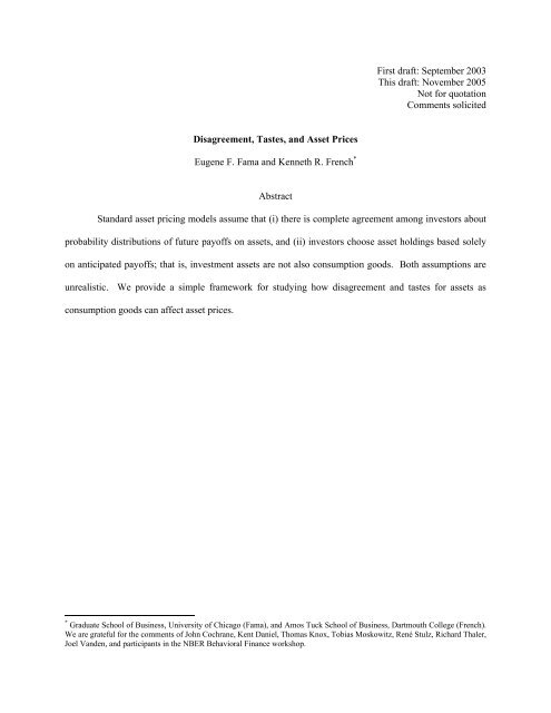
Figure 1 shows the relations among portfolios M, T, and D. The tangency portfolio T is the
portfolio on the true minimum-variance frontier for risky assets with the highest Sharpe ratio,
(3) ST = [E(RT) – RF]/σ(RT),
where E(RT) and σ(RT) are the expected value and standard deviation of the return on T, and RF is the
riskfree rate. Group D investors are misinformed, so portfolio D is not typically the true tangency
portfolio, and the Sharpe ratio SD is less than ST. Since the market portfolio M is a positively weighted
portfolio of T and D, M is between T and D on the hyperbola linking them, and SM is between SD and ST.
In the CAPM, the true tangency portfolio is the market portfolio. When all assumptions of the
CAPM hold except complete agreement – and there is at least one informed and one misinformed investor
(so 0 < x < 1) – equation (1) implies that T is M only if D is also M. In other words, the CAPM holds
only if misinformed investors as a group hold the market portfolio. This can happen when the mistaken
beliefs of the misinformed wash (they are on average correct) or when prices are fully revealing (which
says that, given prices, beliefs are correct). But the message from (1) is that a necessary condition for
CAPM pricing when there is disagreement is that the misinformed in aggregate hold the market portfolio.
The market clearing condition of equation (1) then implies that the informed must also choose M, which
means securities must be priced so that M is the tangency portfolio T. 1
1 If there are no informed investors, securities must be priced so that the aggregate portfolio D of the misinformed is the market
portfolio M. In this case, CAPM pricing holds only when the beliefs of the misinformed are on average correct, so D = M is also
the true tangency portfolio T.
4

B. A More General Perspective
The elegant simplicity of the CAPM makes it an attractive framework for studying the effects of
disagreement on asset prices. But the argument about how disagreement can affect prices centers more
fundamentally on the nature of a market equilibrium. Thus, prices must produce market clearing. This
means prices must induce informed investors (in aggregate) to overweight (relative to market weights) the
assets underweighted by the misinformed due to their erroneous beliefs, and to underweight the assets
overweighted by the misinformed. These actions of the informed tend to offset the price effects of the
misinformed. But when investors are risk averse, the offset is only partial and some of the price effects of
erroneous beliefs typically remain.
Stated this way, our argument is a market equilibrium version of the “limits of arbitrage”
argument of Shleifer and Vishny (1997). The equilibrium perspective does, however, add value. In
particular, it becomes immediate and transparent that when arbitrage is risky, risk averse informed
investors do not fully offset the price effects of the misinformed.
The equilibrium perspective also produces fresh insights. For example, many readers express the
view that the portfolio actions of the informed eventually wipe out the perverse price effects of the
misinformed. Our analysis implies, however, that the price effects of bad beliefs do not disappear in time
unless the beliefs of the misinformed about today’s news converge to the beliefs of the informed.
Without movement by the misinformed, the informed (who always hold the complement of the aggregate
portfolio of the misinformed) have no incentive to take further action that erases the price effects of the
misinformed. For prices to converge to rational values, the misinformed must learn the error of their
ways, so eventually there is complete agreement about old news.
C. Empirical Implications
In principle, one can measure the extent to which prices are irrational. In the CAPM the market
portfolio is the tangency portfolio. Thus, if all CAPM assumptions hold except complete agreement, the
difference between the Sharpe ratio for the true tangency portfolio and the Sharpe ratio for market
5

portfolio, ST - SM, is an overall measure of the effect of misinformed beliefs on asset prices. (The
calibrations presented later provide examples.)
An obvious problem is that we do not know the composition of portfolio T. And the problem is
serious. The power of complete agreement is that, along with the other assumptions of the CAPM, it
allows us to specify that the mean-variance-efficient (MVE) tangency portfolio T is the market portfolio
M. Thus, the composition of T is known. The first-order condition for MVE portfolios, applied to M,
can then be used to specify expected returns on assets – the pricing equation of the CAPM.
Without complete agreement, the assumptions of the CAPM do not suffice to identify T or any
other portfolio that must be on the true MVE boundary. This means that, without complete agreement,
testable predictions about how expected returns relate to risk are also lost. And the problem is not special
to the CAPM. In short, complete agreement is a necessary ingredient of testable asset pricing models –
unless we are willing to specify the nature of the beliefs of the misinformed and exactly how they affect
portfolio choices and prices (for example, De Long, Shleifer, Summers, and Waldmann 1990).
If disagreement is the only potential violation of CAPM assumptions, however, we can use the F-
test of Gibbons, Ross, and Shanken (GRS 1989) to infer whether disagreement indeed affects asset prices.
The GRS test constructs an empirical tangency portfolio using sample estimates of expected returns and
the covariance matrix of returns on the assets in the test, including the market portfolio. The test then
measures whether the tangency portfolio constructed from the full set of assets has a reliably higher
Sharpe ratio than the market portfolio alone (ST > SM). If disagreement is the only potential violation of
CAPM assumptions, the GRS test allows us to infer whether it has measurable effects on asset prices.
Jensen’s (1968) alpha is another measure of deviations from CAPM pricing. Jensen’s alpha is the
deviation of the actual expected return on asset j from its CAPM expected value,
(4) αjM = E(Rj) – {RF + βjM[E(RM) – RF]},
where βjM is the slope in the regression of Rj - RF on RM - RF, and αjM is the intercept.
Unless the misinformed happen to hold the true tangency portfolio T, so T, M, and D coincide,
Jensen’s alpha for T is positive. To see this, divide αTM by the standard deviation of RT,
6

(5)
α ER ( ) −RER ( ) −R
TM
T f M f
= −β = S − ρ(
R , R ) S ,
TM T T M M
σ( R ) σ( R ) σ(
R )
T T T
where ρ(RT, RM) is the correlation between RT and RM. Since the Sharpe ratio for T is greater than the
Sharpe ratio for M and ρ(RT, RM) is less than one, αTM is positive. Moreover, Jensen’s alpha for the
market portfolio, αMM, is zero. Since (10) implies that,
(6) αMM = x αTM + (1 - x) αDM,
we can infer that αDM, Jensen’s alpha for the risky portfolio of misinformed investors, is negative.
In short, when there are misinformed investors whose bad beliefs produce deviations from CAPM
pricing, informed investors have positive values of Jensen’s alpha, and the portfolio decisions of the
misinformed produce negative alphas.
D. Active Management
Among practitioners it is widely believed that active investment managers (stock pickers) help
make prices rational and that prices are less rational if active managers switch to a passive market
portfolio strategy. Indeed, this is often offered as a justification for the existence of active managers,
despite poor performance.
In our model, the price effects of misinformed managers are like those of other misinformed
investors: trading based on bad beliefs makes prices less rational. And the world is a better place (prices
are more rational) when misinformed investors acknowledge their ignorance and switch to a passive
market portfolio strategy. This typically reduces the over- and underweighting of assets that informed
investors must offset. The difference between the tangency portfolio T and the market portfolio M
shrinks and market efficiency improves.
This argument has a striking corollary. If all misinformed investors turn passive and switch to the
market portfolio, asset prices must induce the informed to also hold M. The tangency portfolio T is then
the market portfolio, the CAPM holds, and prices are the rational result of the beliefs of the informed.
Moreover, if all misinformed investors switch to the market portfolio, most of the informed can turn
7

passive and just hold the market. More precisely, when all misinformed investors hold the market
portfolio, complete rationality of prices requires just one active informed investor, who may have
infinitesimal wealth, but whose rational beliefs nevertheless drive asset prices.
In general, however, when active managers have better information, they are among the informed
who partially offset the actions of the misinformed and so make asset prices more rational. Except in the
special case where misinformed investors hold the market portfolio, market efficiency is reduced when
informed investors switch to a passive market portfolio strategy. Because the remaining informed
investors are risk averse, they do not take up all the slack left by newly passive informed investors, and
the misinformed have bigger price effects.
In our model informed investors generate positive values of Jensen’s alpha, and the misinformed
have negative alphas. The performance evaluation literature (for example, Carhart 1997) suggests that,
judged on alphas, the ranks of the informed among active managers are at best thin. Perhaps informed
active managers act like rational monopolists and absorb the expected return benefits of their superior
information with higher fees and expenses. But the performance evaluation literature suggests that the
ranks of the informed remain thin when returns are measured before fees and expenses.
Carhart (1997) is puzzled by his evidence that there are mutual fund managers (about ten percent
of the total number but a smaller fraction of aggregate mutual fund assets) who generate reliably negative
estimates of Jensen’s alpha before fees and expenses. This is a puzzle only if prices are rational so the
misinformed are protected from the adverse price effects of erroneous beliefs. But in our model, if the
misinformed do not in aggregate hold the market portfolio, their beliefs affect prices, and they pay for
their beliefs with negative alphas.
Overall, the performance evaluation literature suggests that it is difficult to distinguish between
informed and misinformed active managers. This is good news about the performance of markets if it
means that informed investors dominate prices, which, as a result, are near completely rational.
Finally, our simple model ignores transaction costs, but it produces insights about their potential
price effects. Because costs deter trading by the misinformed, costs tend to reduce the price effects of
8

erroneous beliefs. But transaction costs also dampen the response of informed investors to the actions of
the misinformed. Since costs impede both the misinformed, who distort prices, and the informed, who
counter the distortions, their net effect on market efficiency is ambiguous.
There is confusion on this point in the literature. For example, going back at least to Miller
(1977), it is often assumed that limits on short-selling make asset prices less rational (for example,
Figlewski 1981, Jones and Lamont 2002, and Chen, Hong, and Stein 2002). In our model, this is true
when all short-selling is by informed investors. But it may be false when short-sale constraints limit the
trades of misinformed investors.
E. Examples
Some examples give life to the analysis. Suppose the assumptions of the CAPM hold except that
there are misinformed investors who underreact to firm-specific news in the way proposed by Daniel,
Hirshleifer, and Subramanyam (1998) to explain momentum and other firm-specific return anomalies.
The misinformed buy too little (relative to market weights) of the assets with positive news and too much
of the assets with negative news. Since all assets must be held, asset prices induce informed investors to
hold the complement (in the sense of (1)) of the portfolio of the misinformed. This complement is the
tangency portfolio T, but it is not the market portfolio M, so we do not get CAPM pricing.
Another behavioral story is that investors do not understand that profitability is mean-reverting.
As a result, investors over-extrapolate past persistent good times or bad times of firms, causing growth
stocks to be overvalued and distressed (value) stocks to be undervalued. Suppose such overreaction is
typical of misinformed investors. Then (given a world where all CAPM assumptions except complete
agreement hold) the misinformed underweight value stocks (relative to market weights) and overweight
growth stocks, and prices must induce the informed to overweight value stocks and underweight growth
stocks. The portfolio of the informed is the true tangency portfolio, but it is not the market portfolio, so
we do not get CAPM pricing. This seems to be the scenario DeBondt and Thaler (1987), Lakonishok,
Shleifer and Vishny (1994), Haugen (1995), and Barberis, Shleifer, and Vishny (1998) have in mind, with
9

the cycle repeating for each new vintage of growth and value stocks, and with the misinformed never
coming to understand their initial overreaction to the past performance of growth and value stocks.
Does asset pricing in a world where the misinformed over-extrapolate the past fortunes of growth
and value stocks move away from the CAPM to a multifactor version of Merton’s (1973) ICAPM?
Generally, the answer is no. In an ICAPM, the market portfolio is not mean-variance-efficient, but it is
multifactor efficient in the sense of Fama (1996). Since the portfolio choices of the misinformed are
based on incorrect beliefs, it is unlikely they produce price effects that put the market portfolio on the
multifactor efficient frontier implied by all currently knowable information.
There is a situation where overreaction and other behavioral biases can lead to an ICAPM, but
one with irrational pricing. This happens when the biases produce expected return effects that are
proportional to covariances of asset payoffs with state variables or common factors in returns. Style
investing may be an example. Thus, defined benefit pension plans often allocate investment funds based
on commonly accepted asset classes (large stocks, small stocks, value stocks, growth stocks, etc.). The
asset classes seem to correspond to common factors in returns (Fama and French 1993). And asset
allocation decisions are often based on exposures to (covariances with) these factors. If plan sponsors do
not choose the market portfolio, their actions can lead to an ICAPM that may be driven by behavioral
biases. For example, the overreaction to the recent past return performance of asset classes proposed by
Barberis and Shleifer (2003), or the overreaction to past profitability and growth proposed by DeBondt
and Thaler (1987), Lakonishok, Shleifer, and Vishny (1994), and Haugen (1995) might produce ICAPM
or near-ICAPM pricing.
II. Tastes for Assets
A common assumption in asset pricing models is that investors are concerned only with the
payoffs from their portfolios; that is, investment assets are not also consumption goods. We provide a
simple analysis of how tastes for assets as consumption goods can affect asset prices. We consider two
10

cases. (i) Utility depends directly on the quantities of assets held. (ii) Tastes for assets are related to the
covariances of asset returns with common return factors or state variables.
A. Tastes for Assets Do Not Depend on Returns
To focus on the effects of tastes, suppose there is complete agreement and asset prices are
rational. Suppose some investors, called group A, evaluate assets based solely on the dollar payoffs and
thus the access to overall consumption they provide. In other words, group A investors have no tastes for
specific assets as consumption goods. Investors who do have such tastes are called group D. Group D
investors get direct utility from their holdings of some assets, above and beyond the utility from general
consumption that the payoffs on the assets provide. 2
Examples are plentiful. “Socially responsible investing” (for example, refusing to hold the stocks
of tobacco companies or gun manufacturers) is an extreme form of tastes for assets as consumption goods
that are unrelated to returns. Another example is loyalty or the desire to belong that leads to utility from
holding the stock of one’s employer (Cohen 2003), one’s favorite animated characters, or one’s favorite
sports team that is unrelated to the payoff characteristics of the stock. The home bias puzzle (French and
Poterba 1991, Karolyi and Stulz 2003), that is, the fact that investors hold more of the assets of their
home country than would be predicted by standard mean-variance portfolio theory, is perhaps another
example. Finally, there may be investors who get pleasure from holding growth stocks and dislike
holding distressed (value) stocks, and these tastes influence investment decisions. This is the thrust of the
characteristics model of Daniel and Titman (1997).
Even when employees do not have tastes for employer stock as a consumption good, options and
grants that constrain an employee to hold the stock for some period of time affect portfolio decisions in
the same way as tastes for the stock. The lock-in effect of capital gains taxes and tax rates on investment
2 Formally, the tastes of an investor i of group D are described by the utility function Ui(C 1, q 1,…, q n, W 2), where C 1 is the dollar
value of time 1 pure consumption goods, q1,…, q n are the dollar investments in the n portfolio assets, W 2 = Σ j q j(1 + R j) is the
wealth at time 2 from investments at time 1, and Σ j q j = W 1 - C 1. Utility need not depend on time 1 holdings of all assets, and the
holdings with zero marginal utility can differ across group D investors. For an investor in group A, utility does not depend on the
time 1 holdings of any assets, and the investor’s utility function is Ui(C 1, W 2).
11

eturns that differ across assets can also affect portfolio decisions and asset prices in much the same way
as tastes for assets as consumption goods.
Market equilibrium in a world where some investors have tastes for assets as consumption goods
is generically like equilibrium in a world where some investors trade based on misinformed beliefs. Thus,
suppose all assumptions of the CAPM hold, except some investors have tastes for assets as consumption
goods. As usual, group A investors (no such tastes) combine the riskfree asset with the true mean-
variance-efficient (MVE) tangency portfolio T of risky assets. A group D investor also combines riskfree
borrowing or lending with a portfolio of risky assets. But the risky portfolio chosen in part depends on
the investor’s tastes for assets, so it is not typically the unconditional tangency portfolio T. Given risk
aversion, however, the investor’s portfolio is conditionally MVE: given the investments in assets with
non-zero marginal utility as consumption goods, the portfolio maximizes expected return given its return
variance and minimizes variance given its expected return.
Market clearing prices require that the market portfolio of risky securities is the aggregate of the
risky portfolios chosen by investors. We can again express this condition as,
(7) wjM = x wjT + (1-x) wjD, j = 1, 2, …, n,
where wjD is the weight of asset j in the wealth-weighted aggregate portfolio of the risky portfolios of
group D investors, and x is the share of group A investors in total wealth invested in risky assets.
As indicated by the choice of symbols, this equilibrium is like the one obtained when deviations
from CAPM pricing are due to misinformed investors. Again, asset prices must induce group A to choose
the complement (in the sense of (7)) of the portfolio of group D. And again, we do not get CAPM pricing
except when the tastes of group D investors are perfectly offsetting and in aggregate they hold the market
portfolio M, so group A investors also hold M, and M must be the tangency portfolio T.
There is one important respect in which price effects induced by tastes may differ from those due
to disagreement. Tastes are exogenous, and there is no economic logic that says tastes for assets as
consumption goods eventually disappear. But economic logic does suggest that the price effects of
12

disagreement are temporary. Misinformed investors should eventually learn they are misinformed and
switch to a passive market portfolio strategy or turn portfolio management over to the informed.
B. Tastes for Assets Depend on Their Returns
If investor utility depends directly on the amounts invested in specific assets, asset prices do not
conform to the CAPM. And prices are unlikely to conform to Merton’s (1973) ICAPM. ICAPM pricing
arises when the utility of time 2 wealth, Ui(C1, W2 | S2), depends on stochastic state variables, S2.
Covariances of time 2 asset returns with the state variables then become an ingredient in portfolio
decisions and asset pricing. In contrast, when utility Ui(C1, q1,…, qn, W2) depends on the quantities of
assets chosen at time 1, q1,…, qn, we do not typically get ICAPM pricing.
ICAPM pricing does arise if investor tastes for assets as consumption goods depend not on the
amount of each asset held, but instead on covariances of asset returns with common return factors or state
variables. This is not, of course, the motivation for the ICAPM in Merton (1973). He emphasizes that the
utility of wealth depends on how it can be used to generate future consumption and on the portfolio
opportunities that will be available to move wealth through time for consumption. Thus, the state
variables, S2, are usually assumed to be related to future consumption and investment opportunities.
As a logical possibility, however, ICAPM pricing can also arise because some state variables or
common factors in returns affect investor utility solely as a matter of tastes. For example, Fama and
French (1993) argue that the value premium is explained by a multifactor version of Merton’s (1973)
ICAPM that includes a value-growth return factor. But this leaves an open issue. Does the value
premium trace to a state variable related to uncertainty about consumption-investment opportunities (the
standard ICAPM story of Fama and French 1993), or to tastes for a return factor related to the value-
growth characteristics of firms (which can be viewed as a variant of the characteristics model of Daniel
and Titman 1997), or to irrational optimism about growth firms and pessimism about value firms
(DeBondt and Thaler 1987, Lakonishok, Shleifer, and Vishny 1994, Haugen 1995)? And the overall
message from these papers is that distinguishing among alternatives is difficult, perhaps impossible.
13

III. Calibrations
Do misinformed investors (or investors who have tastes for assets as consumption goods) have a
big impact on asset prices, or are small price changes enough to induce informed investors to counter the
demands of the misinformed? We use two sets of calibrations to explore this issue. The first examines in
general terms how expected returns move away from the CAPM as one varies (i) the parameters of the
joint distribution of the payoffs on the assets favored and disfavored by the misinformed, and (ii) the
amount of under and overweighting of the two asset groups imposed on the informed. In the second set
of calibrations, we get more specific and use observed small and big stock returns, value and growth stock
returns, and high and low momentum returns to explore how these three prominent CAPM anomalies
distort the tangency portfolio of informed investors. If the anomalies are due to bad beliefs rather than to
the pricing of rational risks, the second set of calibrations captures the resulting price effects, and so
provides perspective on the relative importance of misinformed beliefs in generating the size, value, and
momentum anomalies. The analysis focuses primarily on deviations from CAPM pricing due to
disagreement, but all conclusions apply as well to the price effects of asset tastes.
A. Expected Returns and Misinformed Beliefs: General Factors
The first set of calibrations studies the factors that determine whether the price effects of
misinformed beliefs are large or small. Since the setup and calculations are tedious and the findings are
not controversial, we leave the details to the Appendix. Here we just overview the results and illustrate
them using the value and momentum anomalies of the CAPM.
In a world that otherwise conforms to the assumptions of the CAPM, the price effects of
misinformed beliefs depend most directly on how the tangency portfolio of informed investors differs
from the market portfolio. The distortions of the tangency portfolio held by the informed in turn depend
on (i) their share of invested wealth, and (ii) the extent to which the aggregate portfolio of the
misinformed deviates from the market portfolio. When the informed hold the lion’s share of invested
wealth, large portfolio distortions by the misinformed can leave the portfolio of the informed close to the
14

market portfolio, and the price effects of misinformed beliefs are minor. But when most invested wealth
is controlled by the misinformed, small tilts away from the market portfolio by the misinformed can push
the tangency portfolio of the informed far from the market portfolio and move expected returns far from
the predictions of the CAPM. Similarly, given the wealth shares of informed and misinformed investors,
more extreme portfolio choices by the misinformed increase the gap between the market portfolio and the
tangency portfolio of the informed, and so produce more serious CAPM violations.
The calibrations also say that the price effects of erroneous beliefs are larger the lower is the
correlation between the payoffs on assets over and underweighted by misinformed investors. In the
extreme, if the payoffs on the over and underweighted asset groups are perfectly correlated, the two are
perfect substitutes, so no price changes are needed to induce informed investors to offset the actions of the
misinformed. But lower correlation between the payoffs on the assets over and underweighted by the
misinformed makes diversification more effective, and price effects must be larger to induce the informed
to take the complements of the positions of the misinformed.
We can give life to this correlation result in the context of the value and momentum anomalies of
the CAPM. Lakonishok, Shleifer, and Vishny (1994) and Daniel and Titman (1997) claim that the value
premium (the difference between the expected returns on value and growth stocks) offers a near riskless
arbitrage with a large expected payoff. Fama and French (1993) find, however, that long-short positions
in diversified portfolios of value and growth stocks have large return variances, so they are not close to
riskless arbitrages. The distinction matters. Near riskless arbitrage would imply that the returns on
diversified portfolios of value and growth stocks are near perfectly correlated. Our calibrations then say
that a large value premium is unlikely unless there is a severe dearth of informed investors or severe
restrictions on their portfolio choices. In contrast, if tastes (Daniel and Titman 1997) or bad beliefs
(DeBondt and Thaler 1987, Lakonishok, Shleifer, and Vishny 1994, and Haugen 1995) cause some
investors to underweight value stocks and overweight growth stocks, the relatively low correlation
between value and growth returns documented by Fama and French (1993) can magnify the resulting
15

price effects. Of course, a volatile value-growth spread also opens the possibility that the value premium
is just compensation for risk.
Daniel, Hirshleifer, and Subrahmanyam (1998) posit that the momentum anomaly of Jegadeesh
and Titman (1993) is due to investor underreaction to firm-specific information. By definition, positive
and negative firm-specific information is randomly scattered among firms, so diversified positive and
negative momentum portfolios are likely to be highly correlated. Thus, when there are informed
investors, underreaction to firm specific information should not have large price effects. Moskowitz and
Grinblatt (1999) find, however, that industries are important in momentum. Industry effects are not
diversifiable, and Carhart (1997) confirms that long-short positions in diversified positive and negative
momentum portfolios have substantial return variance, which allows more room for price effects when
there are informed investors.
The final result from the calibrations in the Appendix is that misinformed investors have less
price impact when their bad information is limited to assets that are a small part of the market, so their tilt
away from the market portfolio requires small adjustments by informed investors. This is essentially the
case analyzed by Petajisto (2004), who finds that an exogenous change in the demand for an individual
stock (due, for example, to its addition to the S&P 500) has little impact on prices in a CAPM framework.
But this conclusion presumes that investors are misinformed about (or have specific tastes for) only this
stock; their demands for other stocks are in line with the demands of informed investors.
B. Size, Value, and Momentum
The calibrations discussed above examine the general factors that determine how expected returns
are affected by misinformed beliefs or asset tastes. We now study more specifically what the observed
returns associated with three prominent CAPM anomalies (size, value, and momentum) imply about the
tangency portfolio of informed investors. We interpret the results as potential evidence on the wealth
held by investors who are informed about the behavioral biases that might give rise to the anomalies.
16

Small stocks, with low market capitalizations, tend to have higher average returns than big stocks
(Banz 1981). Suppose this size effect is due to the bad beliefs of misinformed investors or more simply
to asset tastes that cause some investors to overweight big stocks and underweight small stocks. To
examine the impact of the size effect on the tangency portfolio of informed investors, we sort NYSE,
AMEX (after 1962), and Nasdaq (after 1972) firms on their market capitalization (cap) at the beginning
of each year from 1927 to 2004. We allocate stocks accounting for 90% of aggregate market cap to the
big stock portfolio (labeled L for low expected return). The stocks accounting for the remaining 10% of
market cap are in the small stock portfolio (labeled H for high expected return). The 90-10 split is
roughly equivalent to defining big stocks as those above the NYSE median market cap.
The averages, standard deviations, and correlation between the annual value weight returns on the
big (L) and small (H) portfolios are in Table 1. From 1927 to 2004, the average return on the small
portfolio exceeds that on the big portfolio by 4.08% per year, and the correlation between the returns on
the two portfolios is 0.88. If we ignore measurement error and treat the sample means, standard
deviations, and correlation as true parameters, we can infer how much informed investors must
overweight small stocks and underweight big stocks to accommodate the demands of misinformed
investors. Since, aside from disagreement, the assumptions of the CAPM hold, this is equivalent to
asking what combination of H and L produces the tangency portfolio that maximizes the Sharpe ratio.
To derive the weight of portfolio H in the tangency portfolio, we use the standard asset pricing
relation for the tangency portfolio,
(8)
ER ( − R) = β ER ( −R)
H F HT T F
Cov[ RH, wHRH + (1 −wH)
RL] = Ew [ HRH + (1 −wH) RL −RF]
,
Var[ w R + (1 −w)
R ]
H H H L
where βHT = Cov(RH, RT)/Var(RT) is the beta of portfolio H with respect to the tangency portfolio T, wH is
the weight of H in T and 1-wH is the weight of L. Expanding the variance and covariance terms in (8) and
solving for wH yields,
17

(9)
w
H
=
σ ( R ) E( R −R ) −Cov( R , R ) E( R −R
)
2
L H F H L L F
2
[ σ ( RL) −Cov( RH, RL)] E( RH 2
− RF) + [ σ ( RH) −Cov( RH, RL)] E( RL −RF)
where σ 2 (RL) and σ 2 (RH) are return variances.
Using the 1927-2004 parameter estimates in Table 1, 51% of the tangency portfolio of informed
investors is in L, the big stock portfolio, and 49% is in H, the small stock portfolio. Thus, if we ignore
measurement error, the bad beliefs of misinformed investors lead to a tangency portfolio for the informed
that, at least in terms of weights, is far from the market allocation of 90% in big and 10% in small. But
this large difference in portfolio weights produces only a tiny difference between the Sharpe ratios of the
tangency portfolio and the market portfolio. The return on the tangency portfolio has a larger standard
deviation as well as a larger mean (Table 1), and the Sharpe ratio for the tangency portfolio is 0.42, versus
0.40 for the market portfolio. And we argue below that measurement error in our parameter estimates
implies that the tangency portfolio of informed investors is indistinguishable from the market. This result
is in line with more rigorous tests that find that the size effect is consistent with the CAPM (for example,
Chan and Chen 1988, Fama and French 2005).
Our approach to examining how the value premium affects the tangency portfolio of informed
investors is similar to the approach we use for the size effect. At the end of each June from 1926 to 2004,
we sort NYSE, AMEX (after 1962), and Nasdaq (after 1972) firms on the ratio of book equity for the
fiscal year ending in the previous calendar year divided by market equity for December of that year. We
then split aggregate market equity at the end of June equally between a high book-to-market (B/M) value
portfolio (H) and a low B/M growth portfolio (L). Thus, half of total market equity is in the value
portfolio and half is in the growth portfolio when they are formed each year.
For 1927 to 2004, the average return on the value portfolio exceeds the return on the growth
portfolio by 2.31% per year (Table 1), and the correlation between the returns on the two portfolios is
0.86. If we assume the estimates in Table 1 are the true parameters of the joint distribution of H and L
returns, equation (9) implies that the tangency portfolio of informed investors is long about 125% (wH =
1.25) of the value portfolio and short about 25% of the growth portfolio (wL = -0.25). By construction,
18
,

the market portfolio splits equally between the value and growth portfolios. Thus, the point estimates in
Table 1 suggest that, in terms of portfolio weights, the actions of the misinformed push informed
investors far from the market portfolio. It is interesting, however, that because the tangency portfolio has
a higher standard deviation as well as a higher mean than the market portfolio, the large difference in
portfolio weights produces a Sharpe ratio for the tangency portfolio, 0.45, only modestly higher than the
Sharpe ratio for the market portfolio, 0.40.
Momentum returns produce the most extreme tangency portfolio for informed investors. The
procedure we use to construct momentum portfolios is similar to the procedure for value and growth
portfolios, except we reform the momentum portfolios monthly rather than annually. Specifically, we
sort NYSE, AMEX, and Nasdaq stocks at the beginning of month t on their cumulative returns from
month t-12 to month t-2. (We skip month t-1 because of the one month return reversals documented by
Jegadeesh 1990 and Asness 1995.) We then split aggregate market equity equally between a high prior
return portfolio, H, and a low prior return portfolio, L, and compute value weight returns for month t. The
annual momentum returns summarized in Table 1 are compounded monthly returns.
The average annual difference between the high and low momentum returns (H and L) is 5.87%
for 1927-2004. This large spread in average returns and the correlation of 0.89 between H and L returns
combine to produce an extreme tangency portfolio. Based on the point estimates, informed investors take
a short position 2.95 times their total wealth in L and go long 3.95 times their total wealth in H. The
result is a dramatic increase in the Sharpe ratio, from 0.40 for the market to 0.68 for the tangency
portfolio. The standard deviation of the return on the tangency portfolio of the momentum portfolios,
42.47% per year, is more than twice that of the market portfolio, 20.83%, but the average excess return on
the tangency portfolio, an eye popping 28.80% per year, dwarfs the market’s healthy 8.31%.
The tangency portfolios discussed above use estimates of expected returns, standard deviations,
and correlations. Since the estimates have measurement error, it interesting to ask how sensitive the
tangency portfolios are to changes in the inputs. For example, how much do we have to reduce the
19

expected return on H and increase the expected return on L to push the tangency portfolio to the market
portfolio? We use the standard CAPM pricing relation to address this question,
(10)
ER ( L − RF)
βLM
ER ( i − RF) = βiMER
( M − RF)
or
=
ER ( H − RF) βHM
where βiM is the market beta of asset i. Since estimates of expected return are much less precise than
estimates of portfolio betas, we focus attention on the impact of errors in estimates of E(RH) and E(RL).
The estimation errors required to reconcile the size effect with the CAPM are modest. The beta
estimates for 1927-2004 are 0.96 for the big portfolio and 1.30 for the small portfolio, and the ratio of
betas is 0.74 (Table 1). This is close to the ratio of the average annual excess returns, 8.06/12.14 = 0.66.
If the expected annual return on the big portfolio is just 0.51% higher than the 1927-2004 average, and the
expected return on the small portfolio is 0.51% lower than the observed return, the ratio of expected risk
premiums matches the ratio of betas, as required by the CAPM condition (10). This “adjusted” spread
between expected big and small returns, (12.14 – 0.51) – (8.06 + 0.51) = 3.07%, is only 0.6 standard
errors from the observed spread, 4.08%. In short, it is easy to reconcile the size effect with the CAPM.
The changes in expected returns that make the tangency portfolio formed from value and growth
portfolios coincide with the market portfolio are larger, but again statistically modest. The 1927-2004
average excess return on the growth portfolio is 7.49% per year and its beta is 0.98 (Table 1). The value
portfolio’s average excess return is 9.80% and its beta is 1.01. Thus, the ratio of betas is 0.97 and the
ratio of average excess returns is 0.76. One combination of measurement errors that reconciles the two is
a positive error of 0.97% in the average value return and a negative error of -0.97% in the growth return.
Statistically, with these errors the implied spread between E(RH) and E(RL), 0.37%, is 1.67 standard errors
from the 1927-2004 average, 2.31%. We should not infer, however, that the value premium is consistent
with the CAPM. Our calibration is designed to provide perspective on how misinformed beliefs might
affect the tangency portfolio of informed investors. There are more powerful ways to test (and reject) the
CAPM (for example, Fama and French, 2005).
20
,

The measurement errors required to reconcile momentum returns with the CAPM are more
extreme. The annual betas for the low and high momentum portfolios for 1927-2004 are 0.96 and 1.03,
and the average excess returns are 5.62% and 11.48% per year. Thus, the ratio of average excess returns,
0.49, is far from the ratio of betas, 0.93. If the 1927-2004 average return on the low momentum portfolio
is 2.63% below the true expected return and the average return on the high momentum portfolio
overstates the true expected return by the same amount, the tangency portfolio becomes the market
portfolio. But if these adjustments are appropriate, the observed spread between the average returns on H
and L, 5.87% per year, is 4.99 standard errors from the true expected spread, a meager 0.62%.
IV. Conclusions
Our calibrations to identify the general factors that determine the price effects of bad beliefs or
tastes for assets as consumption goods say that distortions of expected returns can be large when (i)
misinformed investors or investors with asset tastes account for substantial invested wealth, (ii) they are
misinformed about or have tastes for a wide range of assets, (iii) they take positions much different from
those of the market portfolio, and (iv) the returns on the assets they underweight are not highly correlated
with the returns on the assets they overweight. Whether in fact the price effects are large, we cannot say.
But we hope we have convinced readers that our market equilibrium approach is a simple way to frame
the price effects of disagreement and tastes.
Our analysis produces other interesting insights. Some examples are:
(i) With our market equilibrium perspective, the limits to arbitrage arguments of Shleifer
and Vishny (1997) are immediate and transparent.
(ii) Offsetting actions by informed investors do not typically suffice to cause the price effects
of bad beliefs to disappear with the passage of time. For prices to converge to rational
values, the beliefs of misinformed investors must converge to those of the informed, so
eventually there is complete agreement about old news.
(iii) Carhart (1997) is puzzled by his evidence that there are mutual fund managers who
generate reliably negative estimates of Jensen’s alpha before fees and expenses. But in
our model, informed investors have positive alphas and the misinformed pay for their bad
beliefs with negative alphas.
21

(iv) It is commonly assumed that lower trading costs make security prices more rational. But
since costs impede both the misinformed, who distort prices, and the informed, who
counter the distortions, the net effect of costs on market efficiency is ambiguous.
(v) Similarly, leaning on Miller (1997), many recent papers argue that restrictions on short
selling lead to less rational prices. But lower costs for short sales can make prices less
rational when short-selling is driven by the erroneous beliefs of misinformed investors.
(vi) The price effects induced by tastes for assets as consumption goods are much like those
due to disagreement. But there is an important difference. Economic logic suggests that
the price effects of disagreement are temporary, as misinformed investors eventually
learn they are misinformed. But tastes are exogenous, and there is no economic logic that
says tastes for assets as consumption goods eventually disappear.
Our calibrations that study more specifically the portfolio allocations imposed on informed
investors by the size, value, and momentum anomalies of the CAPM say that the value premium implies a
more extreme tangency portfolio and more extreme distortions of expected returns than the size effect,
and the tangency portfolio produced by momentum returns is by far most extreme. The correlations
between the High and Low portfolio returns of the three CAPM anomalies are similar, from 0.86 to 0.89,
so the correlations are not a major source of the differences in price effects. If we stick with behavioral
stories for the anomalies, we are left with two potentially complementary possibilities.
First, the relative wealth controlled by the informed may be different for the three anomalies.
Equivalently, the prevalence of the relevant behavioral biases among investors may differ from one
anomaly to the next. Thus, informed investors (who are not subject to excessive optimism about big
stocks and pessimism about small stocks, or who have no outright preference for big stocks over small
stocks) may control sufficient wealth to keep expected returns on small and big stocks close to the
predictions of the CAPM. The more extreme tangency portfolio produced by the value premium
suggests, however, that behavioral biases (for example, the overreaction story of DeBondt and Thaler
1987, Lakonishok, Shleifer and Vishny 1994, and Haugen 1995), or tastes for growth stocks and distastes
for value stocks (Daniel and Titman 1997) may be more prevalent among investors. Finally, the extreme
returns of momentum portfolios and the extreme tangency portfolio produced by these returns suggest
that relatively little wealth is controlled by informed investors who understand momentum, perhaps
22

ecause almost all investors are subject to the underreaction to firm specific information proposed by
Daniel, Hirshleifer, and Subrahmanyam (1998).
The second possibility is that the differences in the price effects associated with the three CAPM
anomalies are to some extent due to differences in the way they distort the portfolio positions of the
misinformed. Perhaps misinformed investors are more mistaken about the relative prospects of value and
growth stocks than about the relative prospects of small and big stocks, and perhaps they are most
mistaken about the relative prospects of high and low momentum stocks.
Our analysis ignores transaction costs, but costs may in part explain the strength of the effects of
behavioral biases that produce deviations from CAPM pricing. Jegadeesh and Titman (1993) emphasize
that exploiting the momentum anomaly involves high turnover and thus high transaction costs that can
substantially deter the offsets that would otherwise be provided by informed investors. In contrast, small
stocks tend to remain small from one year to the next and the turnover of value and growth stocks is much
less extreme than for momentum portfolios (Fama and French 1995).
There is, of course, also controversy about whether the size, value, and momentum anomalies of
the CAPM are due to behavioral biases, or whether prices are in fact rational but the CAPM is the wrong
asset pricing model. For example, Fama and French (1993) argue that the size and value anomalies are
captured by their three-factor ICAPM, and Carhart (1997) is often interpreted as suggesting that adding a
fourth momentum factor brings the momentum anomaly within the purview of rational asset pricing.
Finally, our analysis may provide perspective on the asset pricing information delivered by the
three-factor model of Fama and French (1993) and Carhart’s (1997) four-factor model. It is possible that
disagreement, tastes for assets as consumption goods, and ICAPM state variable risks all play a role in
asset pricing. Whatever the forces generating asset prices, the mean-variance-efficient tangency portfolio
T can always be used, along with the riskfree rate, to describe differences in expected asset returns. In the
Sharpe-Lintner CAPM, T is the market portfolio M. But when asset pricing is affected by disagreement,
asset tastes, and state variable risks, T is no longer M, and theory no longer specifies the composition of
the tangency portfolio. One (perhaps the only) approach to capturing T is to form a set of diversified
23

portfolios that seem to cover observed differences in average returns related to common factors in returns.
If these portfolios span T, they can be used (along with the riskfree rate) to describe differences in
expected asset returns (Huberman and Kandel 1987). And one can be agnostic about whether the
tangency portfolio is not the market portfolio because of disagreement, tastes for assets as consumption
goods, state variable risks, or an amalgam of the three. This may, in the end, be a reasonable view of the
pricing information captured by the three-factor and four-factor models.
Appendix: Calibrations
To explore the price effects of misinformed investors, we compare two equilibria. The first is a
standard CAPM: all investors hold the true tangency portfolio, which then must be the market portfolio.
In the second equilibrium, misinformed investors do not hold the market, and asset prices must induce
informed investors to hold the complement (in the sense of (1)) of the portfolio of the misinformed.
(Everything that follows holds in the scenario where misinformed investors are replaced by investors with
tastes for assets as consumption goods and the informed are replaced by investors with no such tastes.)
We separate assets into two portfolios. Assets the misinformed underweight in the second
equilibrium are in portfolio H, and those they overweight are in portfolio L. To simplify the notation, we
scale H and L so in aggregate the portfolio of informed investors is one unit of each in the CAPM
equilibrium.
We are interested in the effects of disagreement on the cross-section of asset prices. Thus, to
simplify the analysis, we use a reduced form approach and assume that market parameters – the riskfree
rate, RF, and the Sharpe ratio for the tangency portfolio, ST – do not change when the misinformed alter
their weights in H and L. We also assume aggregate investments in the riskfree asset by group A
investors, and by group D, do not change. (Allowing the misinformed to change their investment in the
riskfree asset, with an offsetting adjustment by the informed, adds another variable and another market
clearing condition, but produces no additional insights.)
24

In the first equilibrium, all investors hold the market portfolio and the expected returns on H and
L satisfy the standard CAPM pricing relation,
(A1) E(Ri) – RF = [E(RM) – RF] Cov(Ri, RM) / σ 2 (RM) = ST Cov(Ri, RM) / σ(RM) i = H, L
where RH, RL, RF, and RM are the gross (one plus) returns on portfolios H and L, the riskfree asset, and the
market. Since the market is the tangency portfolio in this equilibrium, we can use the exogenously
specified Sharpe ratio for the tangency portfolio, ST, in the CAPM equation.
In the second equilibrium, informed and misinformed investors are initially endowed with market
portfolios. The misinformed then sell θH units of H and θL units of L to informed investors. Thus, the
informed own φ H = 1+θH units of H and φ L = 1+θL units of L. Since we assume the informed and the
misinformed do not alter their positions in the riskfree asset, informed investors must finance their
purchases of H with sales of L; if θH is positive, θL must be negative. More precisely, if VH and VL are the
market clearing prices per unit of H and L at the time of the trade,
(A2) θHVH + θLVL = 0.
Since T is the tangency portfolio linking the risk free asset and the minimum variance frontier,
the expected excess return on H is,
(A3) E(RH) – RF = [E(RT) – RF] Cov(RH, RT)/σ 2 (RT) = ST Cov(RH, RT)/σ(RT).
Let PH and PL denote the dollar payoffs on portfolios H and L at the end of the period, with
expected values E(PH) and E(PL), standard deviations σH and σL, and correlation ρ. Then the gross return
on portfolio H is RH = PH/VH, and we can rewrite the expected excess return on H as,
25

(A4)
(A5)
ER ( ) − R = S
H F
T
Cov( P / V , φ P + φ P )
H H H H L L
σφ ( P + φP
)
H H L L
2
1/2
S σ ⎡( φσ )
T
H H + φσρ ⎤
H
L L
= ⎢ 2
⎥
V σ ( φ )
H
HPH + φLPL
⎢⎣ ⎥⎦
2 2 2 2 2
S σ ⎡ 2
T H φHσH + φLφHσHσLρ + φLσLρ ⎤
= ⎢ 2 2 2 2
⎥
V
2
H ⎣ φσ H H + φσ L L + φφσσρ
H L H L ⎦
2 2 2
S σ ⎡ φσ (1 − ρ ) ⎤
T H L L
= 1 2
V
⎢ −
⎥
H ⎣ σ ( φ P + φ P )
H H L L ⎦
Solving (A4) for the current price of a unit of H yields,
V
H
2 2 2
EP ( ) Sσ
⎡ φ σ (1 − ρ ) ⎤
H T H L L
= − ⎢1− 2
⎥
R R σ ( φ P + φ P )
F F ⎣ H H L L ⎦
There is a similar equation for the price of a unit of L,
(A6)
V
L
2 2 2
EP ( ) Sσ
⎡ φ σ (1 − ρ ) ⎤
L T L H H
= − ⎢1− 2
⎥
R R σ ( φ P + φ P )
F F ⎣ H H L L ⎦
Equations (A5) and (A6) describe the prices of H and L as functions of: (i) RF and ST, which we
assume are fixed; (ii) the parameters of the joint distribution of the payoffs PH and PL; and (iii) the
quantities of H and L the misinformed decide to sell, θH and θL. (Recall that i φ = 1 + θi.) Using equations
(A2), (A5), and (A6), Figure A1 shows the expected returns on H and L for different values of θH and ρ.
In the figure, we assume the annual riskfree rate is 2% (RF = 1.02); the expected return on the market in
the CAPM equilibrium is 10% (E(RM) = 1.10); and the payoffs on H and L have the same expected value
(E(PH) = E(PL)) and the same standard deviation (σH = σL).
Since the payoffs on H and L have the same expected value and standard deviation, their
expected returns in the CAPM equilibrium are equal to the expected market return, 10%. Figure A1 then
shows that the misinformed can have a big impact on expected returns. For example, if the correlation (ρ)
between H and L is 0.5 and the misinformed underweight H by 50% of informed investors’ initial
(CAPM) holdings (θH = 0.5), the expected return on H increases from 10% to about 11%. The price
26
1/ 2
1/2
1/ 2
.
.
.
1/2

effect is larger for the assets the misinformed overweight. If ρ = 0.5 and θH = 0.5, the expected return on
L falls from 10% to 8.3%.
Two patterns are clear in Figure A1. First, the price effects of erroneous beliefs are larger the
lower is the correlation between the payoffs on H and L. For example, if θH = 0.5, the expected return on
L is 10% for ρ = 1.0, 8.3% for ρ = 0.5, and 5.6% for ρ = 0.0. In economic terms, lower correlation
between the payoffs on H and L makes diversification more effective, and the price of L must increase
more to induce the informed to hold less of it.
The second clear pattern in Figure A1 is the relation between expected returns and the amount of
over- and underweighting forced on informed investors. If the payoffs on H and L are not perfectly
correlated, an increase in θH produces an increase in E(RH) and a decrease in E(RL); the expected return on
H rises to induce informed investors to hold more H and the expected return on L falls to induce them to
give up part of their position in L. Note that it is the size of the position changes forced on informed
investors that matters. Thus, if informed investors have little wealth, small shifts away from the market
portfolio by the misinformed push the tangency portfolio far from the market portfolio (θH and θL are far
from 0) and cause big changes in the expected returns on H and L. On the other hand, if most wealth is in
the hands of the informed, large reallocations by the misinformed have little effect on prices.
Figure A1 is a situation where misinformed investors can have big price effects. The
misinformed have less impact when their bad information is limited to assets that are a small part of the
market, so their shift away from the market portfolio requires small adjustments by informed investors.
For example, suppose bad information is restricted to the assets in portfolio H, but the expected value and
standard deviation of the payoff on L are 100 times those of H. Now H contributes little to the volatility
of the market payoff, and (if we rule out extreme short positions) forcing the informed to overweight H
has little impact on their overall portfolio and on expected returns. For example, using equation (A4), if
the correlation between the payoffs on H and L is 0.5 and θH increases from 0 to 1 (so the informed must
double their holdings of H), the expected return on H increases by only 0.03%, from 5.93% (in the CAPM
equilibrium) to 5.96%. This is essentially the case analyzed by Petajisto (2004), who finds that an
27

exogenous change in the demand for an individual stock has little impact on prices in a CAPM
framework. But this conclusion presumes misinformed investors are misinformed about only this stock;
their demands for other stocks are in line with the demands of informed investors.
28

References
Admati, Anat, 1985, A noisy rational expectations equilibrium for multiple asset securities markets,
Econometrica 53, 629-657.
Asness, Clifford, Robert Krail, and John Liew, 2001, Do hedge funds hedge?, Journal of Portfolio
Management 28, Fall, 6-19.
Banz, Rolf W., 1981, The relationship between return and market value of common stocks, Journal of
Financial Economics 9, 3-18.
Barberis, Nicholas, and Andrei Shleifer, 2003, Style investing, Journal of Financial Economics 68, 161-
199.
Barberis, Nicholas, Andrei Shleifer, and Robert W. Vishny, 1998, A model of investor sentiment, Journal
of Financial Economics 49, 307-343.
Basak, Suleyman, 2003, Asset pricing with heterogeneous beliefs, Working paper, London Business
School, December.
Biais, Bruno, Peter Bossaerts, and Chester Spatt, 2003, Equilibrium asset pricing under heterogeneous
information, working paper, January.
Breeden, Douglas T., 1979, An intertemporal asset pricing model with stochastic consumption and
investment opportunities, Journal of Financial Economics 7, 265-296.
Carhart, Mark M., 1997, On persistence in mutual fund performance, Journal of Finance 52, 57-82.
Chan, K.C., and Nai-fu Chen, 1988, An unconditional asset-pricing test and the role of firms size as and
instrumental variable for risk, Journal of Finance 43, 309-325.
Chen, Joseph, Harrison Hong, and Jeremy C. Stein, 2002, Breadth of ownership and stock returns,
Journal of Financial Economics 66, 171-205.
Cohen, Lauren, 2003, Loyalty based portfolio choice, manuscript, University of Chicago, GSB.
Daniel, Kent, David Hirshleifer, and Avanidhar Subrahmanyam, 1998, Investor psychology and security
market under and overreactions, Journal of Finance 53, 1839-1885
Daniel, Kent, and Sheridan Titman, 1997, Evidence on the characteristics of cross sectional variation in
stock returns, Journal of Finance 52, 1-33.
DeBondt, Werner F. M. and Richard H. Thaler, 1987, Further evidence on investor overreaction and stock
market seasonality, Journal of Finance 42, 557-581.
De Long, J. Bradford, Andrei Shleifer, Lawrence H. Summers, and Robert J. Waldmann, 1990, Noise
trader risk in financial markets, Journal of Political Economy 98, 703-738.
DeMarzo, Peter, and Costis Skiadas, 1998, Aggregation, determinacy, and informational efficiency for a
class of economies with asymmetric information, Journal of Econoomic Theory 80, 123-152.
29

Fama, Eugene F., 1976, Foundations of Finance, New York: Basic Books.
Fama, Eugene F., 1996, Multifactor portfolio efficiency and multifactor asset pricing, Journal of
Financial and Quantitative Analysis 31, 441-465.
Fama, Eugene F. and Kenneth R. French, 1992, The cross-section of expected stock returns, Journal of
Finance 47, 427-465.
Fama, Eugene F., and Kenneth R. French, 1993, Common risk factors in the returns on stocks and bonds,
Journal of Financial Economics 33, 3-56.
Fama, Eugene F. and Kenneth R. French, 1995, Size and book-to-market factors in earnings and returns,
Journal of Finance, 50, 131-156.
Fama, Eugene F., and Kenneth R. French, 2005, The value premium and the CAPM, Journal of Finance,
forthcoming.
Figlewski, Stephen, 1981, The information effects of restrictions on short sales: Some emprirical
evidence, Journal of Financial and Quantitative Analysis 16, 463-476.
French, Kenneth R., and James M. Poterba, 1991, Investor diversification and international equity
markets, American Economic Review 81, 222-226.
Geczy, Christopher C., Robert F. Stambaugh, and David Levin, 2003, Investing in socially responsible
mutual funds, working paper, the Wharton School, University of Pennsylvania.
Gibbons, Michael R., Stephen A. Ross and Jay Shanken, 1989, A test of the efficiency of a given
portfolio, Econometrica 57, 1121-1152.
Haugen, Robert. 1995. The New Finance: The Case against Efficient Markets. Englewood Cliffs, New
Jersey: Prentice Hall.
Huberman, Gur, and Shmuel Kandel, 1987, Mean variance spanning, Journal of Finance 42, 873-888.
Jarrow, Robert, 1980, Heterogeneous expectations, restrictions on short sales and equilibrium prices,
Journal of Finance 35, 1105-111.
Jegadeesh, Narasimhan, 1990, Evidence of predictable behavior of security returns, Journal of Finance
45, 881-898.
Jegadeesh, Narasimhan and Sheridan Titman, 1993, Returns to buying winners and selling losers:
Implications for stock market efficiency, Journal of Finance 48, 65-91.
Jensen, Michael C., 1968, The performance of mutual funds in the period 1945-1964, Journal of Finance
23, 389-416.
Jones, Charles M., and Owen A. Lamont, 2002, Short-sale constraints and stock returns, Journal of
Financial Economics 66, 207-239.
30

Karolyi, Andrew G., and René M. Stulz, 2003, Are financial assets priced globally or locally?,
forthcoming in the Handbook of the Economics of Finance, George Constantindies, Miton Harris,
and René M. Stulz, eds., North Holland, Volume 1B.
Lakonishok, Josef, Andrei Shleifer and Robert W. Vishny, 1994, Contrarian investment, extrapolation,
and risk, Journal of Finance 49, 1541-1578.
Lintner, John, 1965, The valuation of risk assets and the selection of risky investments in stock portfolios
and capital budgets, Review of Economics and Statistics 47, 13-37.
Lintner, John, 1969, The aggregation of investor’s diverse judgments and preferences in competitive
capital markets, Journal of Financial and Quantitative Analysis 4, 347-400.
Lucas, Robert E., Jr., 1978, Asset prices in an exchange economy, Econometrica 46, 1429-1446.
Mayshar, Joram, 1983, On divergence of opinion and imperfections in capital markets, American
Economic Review 73, 114-128.
Merton, Robert C., 1973, An intertemporal capital asset pricing model, Econometrica 41, 867-887.
Miller, Edwin, 1977, Risk, uncertainty, and divergence of opinion, Journal of Finance 32, 1151-1168.
Moskowitz, Tobias J., and Mark Grinblatt, 1999, Do industries explain momentum, Journal of Finance
54, 1249-1290.
Petajisto, Antti, 2004, Why do demand curves for stocks slope down?, working paper, Yale School of
Management.
Rosenberg, Barr, Kenneth Reid, and Ronald Lanstein, 1985, Persuasive evidence of market inefficiency,
Journal of Portfolio Management 11, 9-17.
Rubinstein, Mark, 1974, An aggregation theorem for securities markets, Journal of Financial Economics
1, 225-244.
Sharpe, William F., 1964, Capital asset prices: A theory of market equilibrium under conditions of risk,
Journal of Finance 19, 425-442.
Shleifer, Andrei, and Robert W. Vishny, 1997, The limits of arbitrage, Journal of Finance 52, 35-55.
Stattman, Dennis, 1980, Book values and stock returns, The Chicago MBA: A Journal of Selected Papers
4, 25-45.
Williams, Joseph T., 1977, Capital asset prices with heterogeneous beliefs, Journal of Financial
Economics 5, 219-239.
31

Table 1 – Average Excess Returns and Market Betas for Portfolios Formed on Market Equity, Book to Market Equity, and Prior Returns, 1927-
2004
To form the size portfolios, we sort firms on their market equity (price times shares outstanding) at the beginning of each year from 1927 to 2004,
and assign 90% of the total beginning-of-year market equity to the Big portfolio (L) and 10% to the Small portfolio (H). We then compute annual
value weight returns from January to December. To form the book-to-market equity (B/M) portfolios, we sort firms at the end of each June from
1926 to 2004 on the ratio of book equity for the previous calendar year divided by market equity for December for that year. We then split the
total market equity at the end of June equally between a high B/M Value portfolio (H) and a low B/M Growth portfolio (L), and compute monthly
value weight returns from July to the next June. To form the momentum portfolios, we sort firms at the beginning of each month t, from January
1927 to December 2004, on their cumulative returns from month t-12 to month t-2. We then split the total market equity equally between high (H)
and low (L) prior return portfolios, and compute value weight returns for month t. The annual B/M and momentum returns are compounded
monthly returns for January to December. The data are from CRSP and Compustat and each pair of portfolios contains the NYSE, AMEX (after
1962), and Nasdaq (after 1972) firms with the data required to construct those portfolios. Thus, the size portfolios for year t include all firms with
market equity data at the beginning of t. The B/M portfolios formed in June of t include only firms with positive book equity in the previous
calendar year and market equity for June of t and December of t-1. The excess return for year t is the annual portfolio return minus the
compounded one month T-bill return, from Ibbotson Associates. Beta is the slope from a regression of a portfolio’s annual excess return on the
market’s excess return. The Sharpe ratio is the average annual excess return divided by the annual standard deviation. The tangency portfolio (T)
is the combination of portfolios (big and small, growth and value, or low and high prior returns) that maximizes the Sharpe ratio.
Big (L) vs Small (H) Growth (L) vs Value (H) Low (L) vs High (H) Prior Return
Market L H H-L T L H H-L T L H H-L T
Average Excess Return 8.31 8.06 12.14 4.08 10.05 7.49 9.80 2.31 10.38 5.62 11.48 5.87 28.80
Standard Deviation 20.83 19.99 29.50 15.07 23.91 21.08 21.91 11.53 23.05 20.55 22.00 9.88 42.47
Standard Error 2.22 2.26 3.34 1.71 2.71 2.25 2.34 1.23 2.61 2.19 2.34 1.05 4.81
Sharpe Ratio 0.40 0.40 0.41 0.27 0.42 0.36 0.45 0.20 0.45 0.27 0.52 0.59 0.68
t-statistic 2.39 1.87 5.57
Beta 0.96 1.30 0.34 1.12 0.98 1.01 0.03 1.01 0.96 1.03 0.07 1.24
Standard Error 0.01 0.06 0.07 0.03 0.03 0.04 0.06 0.05 0.03 0.03 0.05 0.18
Weight in Market Portfolio 0.90 0.10 0.50 0.50 0.50 0.50
Weight in Tangency Portfolio 0.49 0.51 -0.25 1.25 -2.95 3.95
Ratio of Average Excess Returns 0.66 0.76 0.49
Ratio of Betas 0.74 0.97 0.93
Correlation of Annual Excess Returns 0.88 0.86 0.89
32

eturn
Expected R
R f
Figure 1-- Investment Opportunities
and Portfolios T, M, and D
T
M
D
Standard Deviation

Expected Return
0.14
0.12
0.10
0.08
0.06
0.04
0.02
Figure A1 -- Expected Return on H and L as Function
of θ H for Different Correlations (ρ) between P H and P L
E(P H) = E(P L), σ H = σ L
Expected Return on H
Expected Return on L
0.0 0.1 0.2 0.3 0.4 0.5 0.6 0.7 0.8 0.9 1.0
θ H
ρ
0.0
0.2
0.4
0.6
0.8
1.0
0.8
0.6
0.4
0.2
0.0