2 Divide and Conquer
2 Divide and Conquer
2 Divide and Conquer

You also want an ePaper? Increase the reach of your titles
YUMPU automatically turns print PDFs into web optimized ePapers that Google loves.
Algorithms Lecture 2: <strong>Divide</strong> <strong>and</strong> <strong>Conquer</strong><br />
2 <strong>Divide</strong> <strong>and</strong> <strong>Conquer</strong><br />
2.1 MergeSort<br />
The control of a large force is the same principle as the control of a few men:<br />
it is merely a question of dividing up their numbers.<br />
— Sun Zi, The Art of War (c. 400 C.E.), translated by Lionel Giles (1910)<br />
Mergesort is one of the earliest algorithms proposed for sorting. According to Knuth, it was suggested<br />
by John von Neumann as early as 1945.<br />
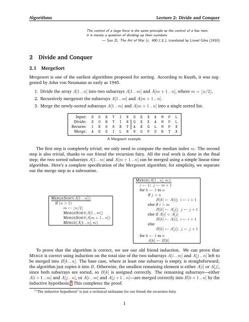
1. <strong>Divide</strong> the array A[1 .. n] into two subarrays A[1 .. m] <strong>and</strong> A[m + 1 .. n], where m = ⌊n/2⌋.<br />
2. Recursively mergesort the subarrays A[1 .. m] <strong>and</strong> A[m + 1 .. n].<br />
3. Merge the newly-sorted subarrays A[1 .. m] <strong>and</strong> A[m + 1 .. n] into a single sorted list.<br />
Input: S O R T I N G E X A M P L<br />
<strong>Divide</strong>: S O R T I N G E X A M P L<br />
Recurse: I N O S R T A E G L M P X<br />
Merge: A E G I L M N O P S R T X<br />
A Mergesort example.<br />
The first step is completely trivial; we only need to compute the median index m. The second<br />
step is also trivial, thanks to our friend the recursion fairy. All the real work is done in the final<br />
step; the two sorted subarrays A[1 .. m] <strong>and</strong> A[m + 1 .. n] can be merged using a simple linear-time<br />
algorithm. Here’s a complete specification of the Mergesort algorithm; for simplicity, we separate<br />
out the merge step as a subroutine.<br />
MERGESORT(A[1 .. n]):<br />
if (n > 1)<br />
m ← ⌊n/2⌋<br />
MERGESORT(A[1 .. m])<br />
MERGESORT(A[m + 1 .. n])<br />
MERGE(A[1 .. n], m)<br />
MERGE(A[1 .. n], m):<br />
i ← 1; j ← m + 1<br />
for k ← 1 to n<br />
if j > n<br />
B[k] ← A[i]; i ← i + 1<br />
else if i > m<br />
B[k] ← A[j]; j ← j + 1<br />
else if A[i] < A[j]<br />
B[k] ← A[i]; i ← i + 1<br />
else<br />
B[k] ← A[j]; j ← j + 1<br />
for k ← 1 to n<br />
A[k] ← B[k]<br />
To prove that the algorithm is correct, we use our old friend induction. We can prove that<br />
MERGE is correct using induction on the total size of the two subarrays A[i .. m] <strong>and</strong> A[j .. n] left to<br />
be merged into B[k .. n]. The base case, where at least one subarray is empty, is straightforward;<br />
the algorithm just copies it into B. Otherwise, the smallest remaining element is either A[i] or A[j],<br />
since both subarrays are sorted, so B[k] is assigned correctly. The remaining subarrays—either<br />
A[i + 1 .. m] <strong>and</strong> A[j .. n], or A[i .. m] <strong>and</strong> A[j + 1 .. n]—are merged correctly into B[k + 1 .. n] by the<br />
inductive hypothesis. 1 This completes the proof.<br />
1 “The inductive hypothesis” is just a technical nickname for our friend the recursion fairy.<br />
1
Algorithms Lecture 2: <strong>Divide</strong> <strong>and</strong> <strong>Conquer</strong><br />
Now we can prove MERGESORT correct by another round of straightforward induction. 2 The<br />
base cases n ≤ 1 are trivial. Otherwise, by the inductive hypothesis, the two smaller subarrays<br />
A[1 .. m] <strong>and</strong> A[m + 1 .. n] are sorted correctly, <strong>and</strong> by our earlier argument, merged into the correct<br />
sorted output.<br />
What’s the running time? Since we have a recursive algorithm, we’re going to get a recurrence<br />
of some sort. MERGE clearly takes linear time, since it’s a simple for-loop with constant work per<br />
iteration. We get the following recurrence for MERGESORT:<br />
T (1) = O(1), T (n) = T ⌈n/2⌉ + T ⌊n/2⌋ + O(n).<br />
2.2 Aside: Domain Transformations<br />
Except for the floor <strong>and</strong> ceiling, this recurrence falls into case (b) of the Master Theorem [CLR,<br />
§4.3]. If we simply ignore the floor <strong>and</strong> ceiling, the Master Theorem suggests the solution T (n) =<br />
O(n log n). We can easily check that this answer is correct using induction, but there is a simple<br />
method for solving recurrences like this directly, called domain transformation.<br />
First we overestimate the time bound, once by pretending that the two subproblem sizes are<br />
equal, <strong>and</strong> again to eliminate the ceiling:<br />
T (n) ≤ 2T ⌈n/2⌉ + O(n) ≤ 2T (n/2 + 1) + O(n).<br />
Now we define a new function S(n) = T (n + α), where α is a constant chosen so that S(n) satisfies<br />
the Master-ready recurrence S(n) ≤ 2S(n/2) + O(n). To figure out the appropriate value for α, we<br />
compare two versions of the recurrence for T (n + α):<br />
S(n) ≤ 2S(n/2) + O(n) =⇒ T (n + α) ≤ 2T (n/2 + α) + O(n)<br />
T (n) ≤ 2T (n/2 + 1) + O(n) =⇒ T (n + α) ≤ 2T ((n + α)/2 + 1) + O(n + α)<br />
For these two recurrences to be equal, we need n/2 + α = (n + α)/2 + 1, which implies that α = 2.<br />
The Master Theorem tells us that S(n) = O(n log n), so<br />
T (n) = S(n − 2) = O((n − 2) log(n − 2)) = O(n log n).<br />
We can use domain transformations to remove floors, ceilings, <strong>and</strong> lower order terms from any<br />
recurrence. But now that we know this, we won’t bother actually grinding through the details!<br />
2.3 QuickSort<br />
Quicksort was discovered by Tony Hoare in 1962. In this algorithm, the hard work is splitting the<br />
array into subsets so that merging the final result is trivial.<br />
1. Choose a pivot element from the array.<br />
2. Split the array into three subarrays containing the items less than the pivot, the pivot itself,<br />
<strong>and</strong> the items bigger than the pivot.<br />
3. Recursively quicksort the first <strong>and</strong> last subarray.<br />
2 Many textbooks draw an artificial distinction between several different flavors of induction: st<strong>and</strong>ard/weak (‘the<br />
principle of mathematical induction’), strong (’the second principle of mathematical induction’), complex, structural,<br />
transfinite, decaffeinated, etc. Those textbooks would call this proof “strong” induction. I don’t. All induction proofs<br />
have precisely the same structure: Pick an arbitrary object, make one or more simpler objects from it, apply the inductive<br />
hypothesis to the simpler object(s), infer the required property for the original object, <strong>and</strong> check the base cases. Induction<br />
is just recursion for proofs.<br />
2
Algorithms Lecture 2: <strong>Divide</strong> <strong>and</strong> <strong>Conquer</strong><br />
Input: S O R T I N G E X A M P L<br />
Choose a pivot: S O R T I N G E X A M P L<br />
Partition: M A E G I L N R X O S P T<br />
Recurse: A E G I L M N O P S R T X<br />
A Quicksort example.<br />
Here’s a more formal specification of the Quicksort algorithm. The separate PARTITION subroutine<br />
takes the original position of the pivot element as input <strong>and</strong> returns the post-partition pivot<br />
position as output.<br />
QUICKSORT(A[1 .. n]):<br />
if (n > 1)<br />
Choose a pivot element A[p]<br />
k ← PARTITION(A, p)<br />
QUICKSORT(A[1 .. k − 1])<br />
QUICKSORT(A[k + 1 .. n])<br />
PARTITION(A[1 .. n], p):<br />
if (p = n)<br />
swap A[p] ↔ A[n]<br />
i ← 0; j ← n<br />
while (i < j)<br />
repeat i ← i + 1 until (i = j or A[i] ≥ A[n])<br />
repeat j ← j − 1 until (i = j or A[j] ≤ A[n])<br />
if (i < j)<br />
swap A[i] ↔ A[j]<br />
if (i = n)<br />
swap A[i] ↔ A[n]<br />
return i<br />
Just as we did for mergesort, we need two induction proofs to show that QUICKSORT is correct—<br />
weak induction to prove that PARTITION correctly partitions the array, <strong>and</strong> then straightforward<br />
strong induction to prove that QUICKSORT correctly sorts assuming PARTITION is correct. I’ll leave<br />
the gory details as an exercise for the reader.<br />
The analysis is also similar to mergesort. PARTITION runs in O(n) time: j − i = n at the<br />
beginning, j − i = 0 at the end, <strong>and</strong> we do a constant amount of work each time we increment i or<br />
decrement j. For QUICKSORT, we get a recurrence that depends on k, the rank of the chosen pivot:<br />
T (n) = T (k − 1) + T (n − k) + O(n)<br />
If we could choose the pivot to be the median element of the array A, we would have k = ⌈n/2⌉,<br />
the two subproblems would be as close to the same size as possible, the recurrence would become<br />
T (n) = 2T ⌈n/2⌉ − 1 + T ⌊n/2⌋ + O(n) ≤ 2T (n/2) + O(n),<br />
<strong>and</strong> we’d have T (n) = O(n log n) by the Master Theorem.<br />
Unfortunately, although it is theoretically possible to locate the median of an unsorted array<br />
in linear time, the algorithm is fairly complicated, <strong>and</strong> the hidden constant in the O() notation is<br />
quite large. So in practice, programmers settle for something simple, like choosing the first or last<br />
element of the array. In this case, k can be anything from 1 to n, so we have<br />
<br />
T (n) = max T (k − 1) + T (n − k) + O(n)<br />
1≤k≤n<br />
In the worst case, the two subproblems are completely unbalanced—either k = 1 or k = n—<strong>and</strong><br />
the recurrence becomes T (n) ≤ T (n − 1) + O(n). The solution is T (n) = O(n 2 ). Another common<br />
heuristic is ‘median of three’—choose three elements (usually at the beginning, middle, <strong>and</strong> end<br />
of the array), <strong>and</strong> take the middle one as the pivot. Although this is better in practice than just<br />
3
Algorithms Lecture 2: <strong>Divide</strong> <strong>and</strong> <strong>Conquer</strong><br />
choosing one element, we can still have k = 2 or k = n − 1 in the worst case. With the medianof-three<br />
heuristic, the recurrence becomes T (n) ≤ T (1) + T (n − 2) + O(n), whose solution is still<br />
T (n) = O(n 2 ).<br />
Intuitively, the pivot element will ‘usually’ fall somewhere in the middle of the array, say between<br />
n/10 <strong>and</strong> 9n/10. This suggests that the average-case running time is O(n log n). Although<br />
this intuition is correct, we are still far from a proof that quicksort is usually efficient. I’ll formalize<br />
this intuition about average cases in a later lecture.<br />
2.4 The Pattern<br />
Both mergesort <strong>and</strong> <strong>and</strong> quicksort follow the same general three-step pattern of all divide <strong>and</strong><br />
conquer algorithms:<br />
1. Split the problem into several smaller independent subproblems.<br />
2. Recurse to get a subsolution for each subproblem.<br />
3. Merge the subsolutions together into the final solution.<br />
If the size of any subproblem falls below some constant threshold, the recursion bottoms out.<br />
Hopefully, at that point, the problem is trivial, but if not, we switch to a different algorithm instead.<br />
Proving a divide-<strong>and</strong>-conquer algorithm correct usually involves strong induction. Analyzing<br />
the running time requires setting up <strong>and</strong> solving a recurrence, which often (but unfortunately not<br />
always!) can be solved using the Master Theorem, perhaps after a simple domain transformation.<br />
2.5 Multiplication<br />
Adding two n-digit numbers takes O(n) time by the st<strong>and</strong>ard iterative ‘ripple-carry’ algorithm, using<br />
a lookup table for each one-digit addition. Similarly, multiplying an n-digit number by a one-digit<br />
number takes O(n) time, using essentially the same algorithm.<br />
What about multiplying two n-digit numbers? At least in the United States, every grade school<br />
student (supposedly) learns to multiply by breaking the problem into n one-digit multiplications<br />
<strong>and</strong> n additions:<br />
31415962<br />
× 27182818<br />
251327696<br />
31415962<br />
251327696<br />
62831924<br />
251327696<br />
31415962<br />
219911734<br />
62831924<br />
853974377340916<br />
We could easily formalize this algorithm as a pair of nested for-loops. The algorithm runs in O(n 2 )<br />
time—altogether, there are O(n 2 ) digits in the partial products, <strong>and</strong> for each digit, we spend constant<br />
time.<br />
We can do better by exploiting the following algebraic formula:<br />
(10 m a + b)(10 m c + d) = 10 2m ac + 10 m (bc + ad) + bd<br />
4
Algorithms Lecture 2: <strong>Divide</strong> <strong>and</strong> <strong>Conquer</strong><br />
Here is a divide-<strong>and</strong>-conquer algorithm that computes the product of two n-digit numbers x <strong>and</strong> y,<br />
based on this formula. Each of the four sub-products e, f, g, h is computed recursively. The last<br />
line does not involve any multiplications, however; to multiply by a power of ten, we just shift the<br />
digits <strong>and</strong> fill in the right number of zeros.<br />
MULTIPLY(x, y, n):<br />
if n = 1<br />
return x · y<br />
else<br />
m ← ⌈n/2⌉<br />
a ← ⌊x/10 m ⌋; b ← x mod 10 m<br />
d ← ⌊y/10 m ⌋; c ← y mod 10 m<br />
e ← MULTIPLY(a, c, m)<br />
f ← MULTIPLY(b, d, m)<br />
g ← MULTIPLY(b, c, m)<br />
h ← MULTIPLY(a, d, m)<br />
return 10 2m e + 10 m (g + h) + f<br />
You can easily prove by induction that this algorithm is correct. The running time for this algorithm<br />
is given by the recurrence<br />
T (n) = 4T (⌈n/2⌉) + O(n), T (1) = 1,<br />
which solves to T (n) = O(n 2 ) by the Master Theorem (after a simple domain transformation).<br />
Hmm. . . I guess this didn’t help after all.<br />
But there’s a trick, first published by Anatoliĭ Karatsuba in 1962. 3 We can compute the middle<br />
coefficient bc + ad using only one recursive multiplication, by exploiting yet another bit of algebra:<br />
ac + bd − (a − b)(c − d) = bc + ad<br />
This trick lets use replace the last three lines in the previous algorithm as follows:<br />
FASTMULTIPLY(x, y, n):<br />
if n = 1<br />
return x · y<br />
else<br />
m ← ⌈n/2⌉<br />
a ← ⌊x/10 m ⌋; b ← x mod 10 m<br />
d ← ⌊y/10 m ⌋; c ← y mod 10 m<br />
e ← FASTMULTIPLY(a, c, m)<br />
f ← FASTMULTIPLY(b, d, m)<br />
g ← FASTMULTIPLY(a − b, c − d, m)<br />
return 10 2m e + 10 m (e + f − g) + f<br />
The running time of Karatsuba’s FASTMULTIPLY algorithm is given by the recurrence<br />
T (n) ≤ 3T (⌈n/2⌉) + O(n), T (1) = 1.<br />
After a domain transformation, we can plug this into the Master Theorem to get the solution T (n) =<br />
O(n lg 3 ) = O(n 1.585 ), a significant improvement over our earlier quadratic-time algorithm. 4<br />
3 However, the same basic trick was used non-recursively by Gauss in the 1800s to multiply complex numbers using<br />
only three real multiplications.<br />
4 Karatsuba actually proposed an algorithm based on the formula (a + c)(b + d) − ac − bd = bc + ad. This algorithm<br />
also runs in O(n lg 3 ) time, but the actual recurrence is a bit messier: a − b <strong>and</strong> c − d are still m-digit numbers, but a + b<br />
<strong>and</strong> c + d might have m + 1 digits. The simplification presented here is due to Donald Knuth.<br />
5
Algorithms Lecture 2: <strong>Divide</strong> <strong>and</strong> <strong>Conquer</strong><br />
Of course, in practice, all this is done in binary instead of decimal.<br />
We can take this idea even further, splitting the numbers into more pieces <strong>and</strong> combining them<br />
in more complicated ways, to get even faster multiplication algorithms. Ultimately, this idea leads<br />
to the development of the Fast Fourier transform, a more complicated divide-<strong>and</strong>-conquer algorithm<br />
that can be used to multiply two n-digit numbers in O(n log n) time. 5 We’ll talk about Fast Fourier<br />
transforms in detail in the next lecture.<br />
2.6 Exponentiation<br />
Given a number a <strong>and</strong> a positive integer n, suppose we want to compute a n . The st<strong>and</strong>ard naïve<br />
method is a simple for-loop that does n − 1 multiplications by a:<br />
SLOWPOWER(a, n):<br />
x ← a<br />
for i ← 2 to n<br />
x ← x · a<br />
return x<br />
This iterative algorithm requires n multiplications.<br />
Notice that the input a could be an integer, or a rational, or a floating point number. In fact,<br />
it doesn’t need to be a number at all, as long as it’s something that we know how to multiply. For<br />
example, the same algorithm can be used to compute powers modulo some finite number (an operation<br />
commonly used in cryptography algorithms) or to compute powers of matrices (an operation<br />
used to evaluate recurrences <strong>and</strong> to compute shortest paths in graphs). All that’s required is that a<br />
belong to a multiplicative group. 6 Since we don’t know what kind of things we’re mutliplying, we<br />
can’t know how long a multiplication takes, so we’re forced analyze the running time in terms of<br />
the number of multiplications.<br />
There is a much faster divide-<strong>and</strong>-conquer method, using the simple formula a n = a ⌊n/2⌋ ·a ⌈n/2⌉ .<br />
What makes this approach more efficient is that once we compute the first factor a ⌊n/2⌋ , we can<br />
compute the second factor a ⌈n/2⌉ using at most one more multiplication.<br />
FASTPOWER(a, n):<br />
if n = 1<br />
return a<br />
else<br />
x ← FASTPOWER(a, ⌊n/2⌋)<br />
if n is even<br />
return x · x<br />
else<br />
return x · x · a<br />
The total number of multiplications is given by the recurrence T (n) ≤ T (⌊n/2⌋) + 2, with the<br />
base case T (1) = 0. After a domain transformation, the Master Theorem gives us the solution<br />
T (n) = O(log n).<br />
5 This fast algorithm for multiplying integers using FFTs was discovered by Arnold Schönhange <strong>and</strong> Volker Strassen in<br />
1971.<br />
6 A multiplicative group (G, ⊗) is a set G <strong>and</strong> a function ⊗ : G × G → G, satisfying three axioms:<br />
1. There is a unit element 1 ∈ G such that 1 ⊗ g = g ⊗ 1 for any element g ∈ G.<br />
2. Any element g ∈ G has a inverse element g −1 ∈ G such that g ⊗ g −1 = g −1 ⊗ g = 1<br />
3. The function is associative: for any elements f, g, h ∈ G, we have f ⊗ (g ⊗ h) = (f ⊗ g) ⊗ h.<br />
6
Algorithms Lecture 2: <strong>Divide</strong> <strong>and</strong> <strong>Conquer</strong><br />
Incidentally, this algorithm is asymptotically optimal—any algorithm for computing a n must<br />
perform Ω(log n) multiplications. In fact, when n is a power of two, this algorithm is exactly optimal.<br />
However, there are slightly faster methods for other values of n. For example, our divide-<strong>and</strong>conquer<br />
algorithm computes a 15 in six multiplications (a 15 = a 7 · a 7 · a; a 7 = a 3 · a 3 · a; a 3 = a · a · a),<br />
but only five multiplications are necessary (a → a 2 → a 3 → a 5 → a 10 → a 15 ). Nobody knows of an<br />
algorithm that always uses the minimum possible number of multiplications.<br />
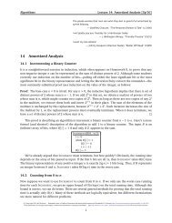
2.7 Optimal Binary Search Trees<br />
This last example combines the divide-<strong>and</strong>-conquer strategy with recursive backtracking.<br />
You all remember that the cost of a successful search in a binary search tree is proportional to<br />
the number of ancestors of the target node. 7 As a result, the worst-case search time is proportional<br />
to the depth of the tree. To minimize the worst-case search time, the height of the tree should be<br />
as small as possible; ideally, the tree is perfectly balanced.<br />
In many applications of binary search trees, it is more important to minimize the total cost of<br />
several searches than to minimize the worst-case cost of a single search. If x is a more ‘popular’<br />
search target than y, we can save time by building a tree where the depth of x is smaller than the<br />
depth of y, even if that means increasing the overall depth of the tree. A perfectly balanced tree<br />
is not the best choice if some items are significantly more popular than others. In fact, a totally<br />
unbalanced tree of depth Ω(n) might actually be the best choice!<br />
This situation suggests the following problem. Suppose we are given a sorted array of n keys<br />
A[1 .. n] <strong>and</strong> an array of corresponding access frequencies f[1 .. n]. Over the lifetime of the search<br />
tree, we will search for the key A[i] exactly f[i] times. Our task is to build the binary search tree<br />
that minimizes the total search time.<br />
Before we think about how to solve this problem, we should first come up with a good recursive<br />
definition of the function we are trying to optimize! Suppose we are also given a binary search tree<br />
T with n nodes; let vi denote the node that stores A[i]. Up to constant factors, the total cost of<br />
performing all the binary searches is given by the following expression:<br />
Cost(T, f[1 .. n]) =<br />
=<br />
n<br />
f[i] · #ancestors of vi<br />
i=1<br />
n<br />
f[i] ·<br />
i=1<br />
n<br />
j=1<br />
<br />
vj is an ancestor of vi<br />
Here I am using the extremely useful Iverson bracket notation to transform Boolean expressions into<br />
integers—for any Boolean expression X, we define [X] = 1 if X is true, <strong>and</strong> [X] = 0 if X is false. 8<br />
Since addition is commutative, we can swap the order of the two summations.<br />
Cost(T, f[1 .. n]) =<br />
n<br />
n<br />
j=1 i=1<br />
f[i] · <br />
vj is an ancestor of vi<br />
Finally, we can exploit the recursive structure of the binary tree by splitting the outer sum into a<br />
sum over the left subtree of T , a sum over the right subtree of T , <strong>and</strong> a ‘sum’ over the root of T .<br />
7<br />
An ancestor of a node v is either the node itself or an ancestor of the parent of v. A proper ancestor of v is either the<br />
parent of v or a proper ancestor of the parent of v.<br />
8<br />
In other words, [X] has precisely the same semantics as !!X in C.<br />
7<br />
(*)
Algorithms Lecture 2: <strong>Divide</strong> <strong>and</strong> <strong>Conquer</strong><br />
Suppose vr is the root of T .<br />
r−1<br />
Cost(T, f[1 .. n]) =<br />
n<br />
j=1 i=1<br />
+<br />
n<br />
i=1<br />
r+1<br />
<br />
+<br />
j=1 i=1<br />
f[i] · <br />
vj is an ancestor of vi<br />
f[i] · <br />
vr is an ancestor of vi<br />
n<br />
f[i] · <br />
vj is an ancestor of vi<br />
We can simplify all three of these partial sums. Since any node in the left subtree is an ancestor<br />
only of nodes in the left subtree, we can change the upper limit of the first inner summation from<br />
n to r − 1. Similarly, we can change the lower limit of the last inner summation from 1 to r + 1.<br />
Finally, the root vr is an ancestor of every node in T , so we can remove the bracket expression from<br />
the middle summation.<br />
r−1<br />
Cost(T, f[1 .. n]) =<br />
r<br />
j=1 i=1<br />
+<br />
n<br />
f[i]<br />
i=1<br />
r+1<br />
<br />
+<br />
j=1 i=r+1<br />
f[i] · <br />
vj is an ancestor of vi<br />
n<br />
f[i] · <br />
vj is an ancestor of vi<br />
Now the first <strong>and</strong> third summations look exactly like our earlier expression (*) for Cost(T, f[1 .. n]).<br />
We finally have our recursive definition!<br />
Cost(T, f[1 .. n]) = Cost(left(T ), f[1 .. r − 1]) +<br />
n<br />
f[i] + Cost(right(T ), f[r + 1 .. n])<br />
The base case for this recurrence is, as usual, n = 0; the cost of the empty tree, over the empty set<br />
of frequency counts, is zero.<br />
Now our task is to compute the tree Topt that minimizes this cost function. Suppose we somehow<br />
magically knew that the root of Topt is vr. Then the recursive definition of Cost(T, f) immediately<br />
implies that the left subtree left(Topt) must be the optimal search tree for the keys A[1 .. r − 1] <strong>and</strong><br />
access frequencies f[1 .. r − 1]. Similarly, the right subtree right(Topt) must be the optimal search<br />
tree for the keys A[r + 1 .. n] <strong>and</strong> access frequencies f[r + 1 .. n]. Once we choose the correct key<br />
to store at the root, the Recursion Fairy will automatically construct the rest of the optimal<br />
tree for us. More formally, let OptCost(f[1 .. n]) denote the total cost of the optimal search tree for<br />
the given frequency counts. We immediately have the following recursive definition.<br />
OptCost(f[1 .. n]) = min<br />
1≤r≤n<br />
<br />
i=1<br />
OptCost(f[1 .. r − 1]) +<br />
n<br />
<br />
f[i] + OptCost(f[r + 1 .. n])<br />
Again, the base case is OptCost(f[1 .. 0]) = 0; the best way to organize zero keys, given an empty<br />
set of frequencies, is by storing them in the empty tree!<br />
8<br />
i=1
Algorithms Lecture 2: <strong>Divide</strong> <strong>and</strong> <strong>Conquer</strong><br />
This recursive definition can be translated mechanically into a recursive algorithm, whose running<br />
time T (n) satisfies the recurrence<br />
T (n) = Θ(n) +<br />
n <br />
T (k − 1) + T (n − k) .<br />
k=1<br />
The Θ(n) term comes from computing the total number of searches n i=1 f[i]. The recurrence<br />
looks harder than it really is. To transform it into a more familiar form, we regroup <strong>and</strong> collect<br />
identical terms, subtract the recurrence for T (n − 1) to get rid of the summation, <strong>and</strong> then regroup<br />
again.<br />
n−1 <br />
T (n) = Θ(n) + 2 T (k)<br />
k=0<br />
n−2 <br />
T (n − 1) = Θ(n − 1) + 2 T (k)<br />
k=0<br />
T (n) − T (n − 1) = Θ(1) + 2T (n − 1)<br />
T (n) = 3T (n − 1) + Θ(1)<br />
The solution T (n) = Θ(3 n ) now follows from the annihilator method.<br />
It’s worth emphasizing here that our recursive algorithm does not examine all possible binary<br />
search trees. The number of binary search trees with n nodes satisfies the recurrence<br />
n−1 <br />
N(n) = N(r − 1) · N(n − r), N(0) = 1,<br />
r=1<br />
which has the closed-from solution N(n) = Θ(4 n / √ n). Our algorithm saves considerable time<br />
by searching independently for the optimal left <strong>and</strong> right subtrees. A full enumeration of binary<br />
search trees would consider all possible pairings of left <strong>and</strong> right subtrees; hence the product in the<br />
recurrence for N(n).<br />
9
Algorithms Lecture 2: <strong>Divide</strong> <strong>and</strong> <strong>Conquer</strong><br />
Exercises<br />
1. Most graphics hardware includes support for a low-level operation called blit, or block transfer,<br />
which quickly copies a rectangular chunk of a pixel map (a two-dimensional array of pixel<br />
values) from one location to another. This is a two-dimensional version of the st<strong>and</strong>ard C<br />
library function memcpy().<br />
Suppose we want to rotate an n × n pixel map 90 ◦ clockwise. One way to do this, at least<br />
when n is a power of two, is to split the pixel map into four n/2 × n/2 blocks, move each<br />
block to its proper position using a sequence of five blits, <strong>and</strong> then recursively rotate each<br />
block. Alternately, we could first recursively rotate the blocks <strong>and</strong> then blit them into place.<br />
A B<br />
C D<br />
C A<br />
D B<br />
B D<br />
A C<br />
A B<br />
C D<br />
Two algorithms for rotating a pixelmap.<br />
Black arrows indicate blitting the blocks into place; white arrows indicate recursively rotating the blocks.<br />
The first rotation algorithm (blit then recurse) in action.<br />
(a) Prove that both versions of the algorithm are correct when n is a power of two.<br />
(b) Exactly how many blits does the algorithm perform when n is a power of two?<br />
(c) Describe how to modify the algorithm so that it works for arbitrary n, not just powers of<br />
two. How many blits does your modified algorithm perform?<br />
(d) What is your algorithm’s running time if a k × k blit takes O(k 2 ) time?<br />
(e) What if a k × k blit takes only O(k) time?<br />
10
Algorithms Lecture 2: <strong>Divide</strong> <strong>and</strong> <strong>Conquer</strong><br />
2. (a) Prove that the following algorithm actually sorts its input.<br />
STUPIDSORT(A[0 .. n − 1]) :<br />
if n = 2 <strong>and</strong> A[0] > A[1]<br />
swap A[0] ↔ A[1]<br />
else if n > 2<br />
m = ⌈2n/3⌉<br />
STUPIDSORT(A[0 .. m − 1])<br />
STUPIDSORT(A[n − m .. n − 1])<br />
STUPIDSORT(A[0 .. m − 1])<br />
(b) Would STUPIDSORT still sort correctly if we replaced m = ⌈2n/3⌉ with m = ⌊2n/3⌋?<br />
Justify your answer.<br />
(c) State a recurrence (including the base case(s)) for the number of comparisons executed<br />
by STUPIDSORT.<br />
(d) Solve the recurrence, <strong>and</strong> prove that your solution is correct. [Hint: Ignore the ceiling.]<br />
Does the algorithm deserve its name?<br />
<br />
.<br />
(e) Prove that the number of swaps executed by STUPIDSORT is at most n<br />
2<br />
3. (a) Suppose we are given two sorted arrays A[1 .. n] <strong>and</strong> B[1 .. n] <strong>and</strong> an integer k. Describe<br />
an algorithm to find the kth smallest element in the union of A <strong>and</strong> B in Θ(log n) time.<br />
For example, if k = 1, your algorithm should return the smallest element of A ∪ B; if<br />
k = n, your algorithm should return the median of A ∪ B.) You can assume that the<br />
arrays contain no duplicate elements. [Hint: First solve the special case k = n.]<br />
(b) Now suppose we are given three sorted arrays A[1 .. n], B[1 .. n], <strong>and</strong> C[1 .. n], <strong>and</strong> an<br />
integer k. Describe an algorithm to find the kth smallest element in A in O(log n) time.<br />
(c) Finally, suppose we are given a two dimensional array A[1 .. m][1 .. n] in which every row<br />
A[i][ ] is sorted, <strong>and</strong> an integer k. Describe an algorithm to find the kth smallest element<br />
in A as quickly as possible. How does the running time of your algorithm depend on m?<br />
[Hint: It is possible to find the kth smallest element in an unsorted array in linear time.]<br />
4. (a) Describe <strong>and</strong> analyze an algorithm to sort an array A[1 .. n] by calling a subroutine<br />
SQRTSORT(k), which sorts the subarray A k + 1 .. k + √ n in place, given an arbitrary<br />
integer k between 0 <strong>and</strong> n− √ n as input. (To simplify the problem, assume that √ n is an<br />
integer.) Your algorithm is only allowed to inspect or modify the input array by calling<br />
SQRTSORT; in particular, your algorithm must not directly compare, move, or copy array<br />
elements. How many times does your algorithm call SQRTSORT in the worst case?<br />
(b) Prove that your algorithm from part (a) is optimal up to constant factors. In other words,<br />
if f(n) is the number of times your algorithm calls SQRTSORT, prove that no algorithm<br />
can sort using o(f(n)) calls to SQRTSORT.<br />
(c) Now suppose SQRTSORT is implemented recursively, by calling your sorting algorithm<br />
from part (a). For example, at the second level of recursion, the algorithm is sorting<br />
arrays roughly of size n1/4 . What is the worst-case running time of the resulting sorting<br />
algorithm? (To simplify the analysis, assume that the array size n has the form 22k, so<br />
that repeated square roots are always integers.)<br />
11
Algorithms Lecture 2: <strong>Divide</strong> <strong>and</strong> <strong>Conquer</strong><br />
5. You are at a political convention with n delegates, each one a member of exactly one political<br />
party. It is impossible to tell which political party any delegate belongs to; in particular,<br />
you will be summarily ejected from the convention if you ask. However, you can determine<br />
whether any two delegates belong to the same party or not by introducing them to each<br />
other—members of the same party always greet each other with smiles <strong>and</strong> friendly h<strong>and</strong>shakes;<br />
members of different parties always greet each other with angry stares <strong>and</strong> insults.<br />
(a) Suppose a majority (more than half) of the delegates are from the same political party.<br />
Describe an efficient algorithm that identifies a member (any member) of the majority<br />
party.<br />
(b) Now suppose exactly k political parties are represented at the convention <strong>and</strong> one party<br />
has a plurality: more delegates belong to that party than to any other. Present a practical<br />
procedure to pick a person from the plurality political party as parsimoniously as<br />
possible. (Please.)<br />
c○ Copyright 2007 Jeff Erickson. Released under a Creative Commons Attribution-NonCommercial-ShareAlike 2.5 License (http://creativecommons.org/licenses/by-nc-sa/2.5/)<br />
12