FODITS - Institut für Astronomische und Physikalische Geodäsie ...

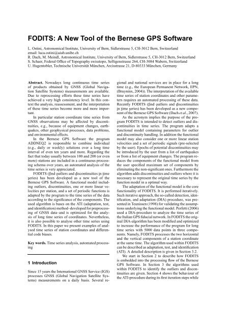
FODITS: A New Tool of the Bernese GPS Software
L. Ostini, Astronomical Institute, University of Bern, Sidlerstrasse 5, CH-3012 Bern, Switzerland
email: luca.ostini@aiub.unibe.ch
R. Dach, M. Meindl, Astronomical Institute, University of Bern, Sidlerstrasse 5, CH-3012 Bern, Switzerland
S. Schaer, Federal Office of Topography swisstopo, Seftigenstrasse 264, CH-3084 Wabern, Switzerland
U. Hugentobler, Technische Universität München, Arcisstrasse 21, D-80333 München, Germany
Abstract. Nowadays long continuous time series
of products obtained by GNSS (Global Navigation
Satellite Systems) measurements are available.
Due to reprocessing efforts these time series have
achieved a very high consistency level. In this context
the analysis, reassessment, and the interpretation
of these time series become more and more important.
In particular station coordinate time series from
GNSS observations may be affected by discontinuities,
e.g., because of equipment changes, earthquakes,
other geophysical processes, data problems,
and environmental effects.
In the Bernese GPS Software the program
ADDNEQ2 is responsible to combine individual
(e.g., daily or weekly) solutions over a long time
interval of even ten years and more. Regarding the
fact that today usually between 100 and 200 (or even
more) stations are included in a continuous processing
schema over years, an automated analysis of the
time series is very appreciated.
FODITS (f ¯ ind ōutliers and d ¯ iscontinuities īn t ¯ ime
s ¯ eries) has been developed as a new tool of the
Bernese GPS Software. A functional model including
outliers, discontinuities, one or more linear velocities
per station, and a set of periodic functions is
adapted by the program to the time series of the data
according to the significance of the components. The
used algorithm is bases on the ATI (adaptation, test,
and identification) method–developed for preprocessing
of GNSS data–and is optimized for the analysis
of long time series of coordinates. Nevertheless,
it is also possible to analyse other time series using
FODITS. In this paper we present examples of analysed
time series of station coordinates and differential
code biases.
Key words. Time series analysis, automated processing
1 Introduction
Since 15 years the International GNSS Service (IGS)
processes GNSS (Global Navigation Satellite Systems)
measurements on a daily basis. Several re-
gional and national services are in place for a long
time (e.g., the European Permanent Network, EPN,
(Bruyninx, 2004)). The interpretation of the available
time series of station coordinates and other parameters
requires an automated processing of these data.
Recently FODITS (find ōutliers and discontinuities i
¯ ¯
¯ n t ¯ ime series) has been developed as a new component
of the ¯ Bernese GPS Software (Dach et al., 2007).
As the acronym implies the purpose of the program
FODITS is intended to detect outliers and discontinuities
in time series. The program adapts a
functional model containing parameters for outlier
and discontinuity handling. In addition the functional
model may also consider one or more linear station
velocities and a set of periodic signals (pre-selected
by the user). Epochs of potential discontinuities may
be introduced by the user from a list of earthquakes
or from a list of equipment changes. The program reduces
the components of the functional model from
the user specified maximum set of components by
eliminating the non-significant ones. Furthermore the
algorithm adds discontinuities and outliers where it is
necessary to represent the original time series by the
function model in a optimal way.
The adaptation of the functional model is the core
functionality of FODITS. It is performed iteratively.
Such iterative approach, the so-called detection, identification,
and adaptation (DIA) procedure, was presented
in Teunissen (1998) for validating the assumptions
underlying the functional model. Perfetti (2006)
used a DIA-procedure to analyze the time series of
the Italian GPS fiducial network. In FODITS the original
DIA-algorithm has been modified and optimized
to increase the performance of the program for long
time series with 5000 data points in three components.
Namely, FODITS processes the two horizontal
and the vertical components of a station coordinate
at the same time. The algorithm used within FODITS
can be described as adaptation, test, and identification
(ATI). A detailed description is given in Section 3.2.
We start in Section 2 to describe how FODITS
is embedded into the processing flow of the Bernese
GPS Software. In Section 3 the algorithms used
within FODITS to identify the outliers and discontinuities
are given. Section 4 shows the behaviour of
the ATI-procedure during its first iteration steps while

analyzing CODE (Center for Orbit Determination in
Europe) coordinate time series. The paper gives examples
for processed weekly coordinate time series
for some of the stations in the EPN in Section 5.1.
Section 5.2 illustrates an example of the reassessment
of CODE global daily station coordinate time series.
The analysis of the P1-P2 DCB (Differential Code
Biases) is presented as an example for the processing
of non-coordinate one-dimensional time series in
Section 5.3. A summary is given in Section 6.
2 Description of FODITS and its
Embedding in the Bernese GPS
Software
Time series of coordinates may be represented as a set
of coordinate files resulting from the processing of individual
sessions (e.g., hourly, daily, or even weekly
processing scheme). Introducing the coordinates directly
we have to presume a consistent definition of
the geodetic datum. Alternatively, series of coordinates
may be generated by ADDNEQ2 (combining
the normal equations of the individual solutions from
so-called NEQ-Files) with a consistent datum definition
(represented by the coordinates and velocities as
well as a selection list of the reference frame sites).
In that case the coordinates of the individual solution
may be reconstructed from the resulting station coordinates
and velocities (CRD/VEL) in conjunction
with the residuals of the individual contributing normal
equation files with respect to the combined solution
(PLT). In both cases the variance-covariance information
of the individual coordinate solutions may
be considered.
Figure 1 illustrates the embedding of FODITS in
the Bernese GPS Software.
CRD
Predefined
events
STA
ERQ
EVL
NEQ
Select
EVL VEL CRD
FODITS results
CRD VEL STA
ADDNEQ2
CRD VEL PLT
FODITS
FIX
( )
COV
CRD VEL STA FIX
Updated inputs for ADDNEQ2
File abbreviations:
- EVL: Event list
- ERQ: Earthquake list
- NEQ: Normal equations
- CRD: Coordinates
- VEL: Velocities
- STA: Station information
- FIX: List of reference sites
- PLT: Residual time series
- COV: Variance-covariance
Figure 1. Embedding of FODITS in Bernese GPS Software.
Events of potential discontinuities that shall be
tested by FODITS for their significance are given
with the information on the used equipment for each
station (STA) and a list of earthquakes (ERQ) extracted
from an external database, e.g., U.S. Geological
Survey Earthquake Hazards Program (U.S.G.S.,
2008). It is also possible to enforce the program to
set a discontinuity at dedicated epochs and to setup a
certain set of periodic functions in any case–even if
they are not significant. These predefined events are
introduced by a so-called event list file (EVL). Apart
from the program output, FODITS provides the list
of outliers and discontinuities in a station information
file that can directly be introduced into ADDNEQ2 to
generate the updated (final) time series of station coordinates.
In addition the list of reference frame sites
is adapted according to the detected discontinuities.
3 Functionality of FODITS
FODITS allows the analysis of time series up to three
components. GNSS station coordinate time series are
in fact analysed and modelled in their local components
(North, East, and Up). The space variancecovariance
information of coordinates (exported from
ADDNEQ2 through PLT and COV files, see Figure 1)
flows into the least squares adjustment (LSA) if they
are available. The temporal variance-covariance information
is not taken into account in FODITS.
3.1 The Functional Model
For each station j = 1, . . .,nq we define the functional
model y j(ti) consisting of a number of i =
1, . . .,nt,j epochs. The functional model is independently
derived for each station. For that reason and to
improve the readability of the formulas we do not use
the station index j.
The functional model may consist of a set or a
subset of the following components:
– station coordinates c0 at an epoch t0,
– one or more station velocitiesvk(ti−t0)·ηv,k(ti),
– a number of discontinuities dk · ηd,k(ti),
– a list of outliers sk · ηs,k(ti), and
– a set of periodic functions pk with the predefined
frequency fk and the parameters ak and bk:
y(ti) = c0+ (1)
nv
vk(ti − tv,k) · ηv,k(ti) +
k=1
nd
ns
dk · ηd,k(ti) + sk · ηs,k(ti) +
k=1
k=1
np
[ak sin(2πfkti) + bk cos(2πfkti)] · ηp,k(ti).
k=1

The functions ηv,k(ti), ηd,k(ti), ηs,k(ti) and ηp,k(ti)
are either 0 or 1 to indicate the validity of the corresponding
component for the epoch ti. The total number
of discontinuity, outlier, velocity intervals, and
periodic functions are defined by the variables nd, ns,
nv, and np respectively.
The elements of the coordinate time series are
used as pseudo-observations to estimate the parameters
of the functional model. All three components of
a coordinate time series may be processed together.
Instead of station coordinates also other time series
can be introduced to compute functional models.
3.2 The ATI-procedure
The Nassi-Shneiderman diagram (norm DIN-66261)
of FODITS is shown in Figure 2. The time series pro-
Read CRD or CRD VEL PLT
Input Time Series file(s)
Read EVL ERQ STA
Predefined events
Loop over all time series (=over all stations)
Loop find the most probable discontinuity (interation step loop)
Adapt the model with all known events (=parameters)
Parameter estimation by least square adjustment
Test the significance of all parameters set up in the model
No
( COV )
Loop model screening (screening step loop)
Velocities handling (test and merge)
Remove the all non-significant
parameters and the most
non-significant except
the most probable discontinuitiy
(6.)
Are all parameters in the model
significant?
Yes
Yes
Was the most probable
discontinuity
significant?
Exit the Loop
model screening
Find the most probable discontinuity in the time series
Find all probable outliers in the time series
Write CRD VEL PLT EVL OUT Result files
Write CRD VEL STA FIX
Update ADDNEQ2 input files
(1.)
(2.)
(3.)
(11.)
(4.)
(8.)
(5.)
(6.)
(7.)
No
Exit the Loop find
the most probable
discontinuity (12.)
Figure 2. The Nassi-Shneiderman diagram of FODITS.
(9.)
(10.)
(13.)
(14.)
cessing in FODITS may be divided by the following
steps:
1. The coordinate time series are read either from a
list of coordinate files (CRD) or are reconstructed
from the residuals (PLT) in conjunction with the
resulting coordinate and velocities (CRD/VEL)
from the combination of normal equations in the
ADDNEQ2 program. The variance-covariance
information of the coordinate time series may
be provided in a result variance-covariance file
(COV) and in the residual file (PLT).
2. A list of predefined events like, e.g., equipment
changes (from the station information file, STA)
and earthquakes (ERQ), is generated from the input
files. All these events will be tested in step 6
whether they cause significant discontinuities or
not. Components of the functional model can be
introduced by the user (EVL file). There are three
opportunities to influence the procedure: The resulting
functional model will contain these components
independent from their significance. The
components can be introduced as a proposal that
are verified during the processing for their significance.
Specific components of the default functional
model can be suppressed during specific intervals.
3. FODITS analyzes one station at a time and considers
each station independent from the others.
4. A first functional model is defined. It contains
parameters for all predefined events for this station
taken from step 2. In addition, the parameters
for the user-defined periodic functions are set up.
Moreover, a new velocity parameter is set up after
each earthquake event unless alternative userdefined
configuration (no velocities, only one velocity,
or a new velocity parameter after each discontinuity
parameter) is given.
5. The parameters of the functional model are estimated
by LSA using the elements of the time
series as the pseudo-observations.
6. All parameters of the functional model are tested
for significance. All non-significant parameters
are removed from the functional model step-bystep.
7. Velocity changes are tested for significance. Nonsignificant
velocity changes due to earthquakes
are removed from the functional model if userdefined.
8. All possible velocity changes are reconsidered.
The steps 5., 6., and 7. are repeated until no
more non-significant parameters are included in
the functional model.
9. The epoch of the most probable discrepancy between
the time series and the functional model
is identified that can be fixed by a discontinuity.
A new discontinuity is added to the functional
model at this epoch.
10. Probable outliers are identified and also added to
the functional model.
11. The full functional model with all components
described in step 4. together with the new identified
discontinuity and outliers is setup. The procedure
is repeated from step 5.
12. The iterative procedure terminates if the last identified
most probable discontinuity is removed
from the functional model in step 6. because it
is not significant anymore.

13. Result and output files are generated.
14. Input files for ADDNEQ2 are updated.
In summary the algorithm consists of adaptation (step
4.), test (step 6.), and identification (steps 9. and
10.) (ATI) steps. The progress of the algorithm can
be given in terms of screening and iteration steps: a
screening step (adaptation and test steps of the ATIprocedure)
is completed with the handling of velocities
(step 7.) while an iteration (identification step of
the ATI-procedure) is completed with the search for
probable outliers (step 10.) (see Figure 2).
There is an important advantage in setting up
the full functional model and removing the nonsignificant
elements. The most computer time consuming
part is the setup of the components of the
functional model from the pseudo-observations, the
elements of the time series, e.g., coordinates. So it
is preferable if only components need to be removed
and no parameters for a new component of the functional
model has to be added within one iteration step:
the removal can be done on normal equation level
whereas adding new parameters requires a reprocessing
of the complete time series. This significantly increases
the speed of the program.
3.3 Tests of Significance
We verify the significance of all estimated parameters
x = {d,s,p} by the following statistical test:
Tx =
m0
|x|
TQxx(x,x)T
< u1− α
T 2
, (2)
where m0 is the unit weight of the LSA, Qxx(x,x)
is the cofactor matrix of the parameter x, and T is the
transformation matrix of the operation. Moreover, we
have the critical value u1− α of the normal distribu-
2
tion for a user-defined significance level α.
Let’s add two remarks to the significance tests:
First, for periodic functions we test for the significance
of the amplitude. Second, a minimum size of a
detectable discontinuity (|x| > κd · m0) and outlier
(|x| > κs · m0) is specified in relation to the noise
level of the time series and as an absolute threshold
for the horizontal (|xh| > hd, |xh| > hs) and vertical
(|xv| > vd, |xv| > vs) components. In this way, the
computation time can be significantly reduced, and
the user has a better control of the algorithm (e.g.,
events with a size below 1 mm might be detected as
significant in the time series of very good stations,
what makes from the general experience of the GNSS
processing no sense anymore).
3.4 Searching for New Discontinuities
The removal of the most probable discrepancy (in
terms of discontinuity) between the functional model
and the time series requires the identification of the
epoch of such potential discontinuity. In FODITS, the
identification of this epoch is based on the analysis
of the time series residuals with respect to the recent
functional model
v(ti) = y(ti) − Ax(ti), (3)
where A is the design matrix of the updated functional
model.
Because the original statistical test for the identification
step in the DIA-procedure as proposed in
(Teunissen, 1998) is very computer time consuming,
we have implemented a simplified algorithm to detect
the epoch of the most probable discontinuity discrepancy
at
td in a way that g(td) = maxg(ti) (4)
with
g(ti) =
i
w(tk) , where i = 1, . . .,nt. (5)
k=1
The residual time series
w(ti) = v(ti) − A2x(ti) (6)
is obtained by fitting a first degree polynomial function
(described by the design matrix A2) to the original
residual time series v(ti) (see Eq. 3) with the
peculiarity of resampling the time information with
ti = i for i = 1, · · · , nt.
Let’s add a remark to the test time series of Eq. 5:
by employing the residual time series w(ti) (see
Eq. 6) instead of the original residual time series
v(ti) (see Eq. 3) we make the identification step robust
with respect to the data gaps in the time series
(not unusual for time series derived from GNSS data).
3.5 Searching for Additional Outliers
All residuals of Eq. 3 that fulfill
|v(ti)| > κsm0 and (7)
|vh(ti)| > hs or |vv(ti)| > vs
are identified as outliers. Outliers will be added to
the functional model and tested for significance in the
next iteration step of the ATI-procedure.
3.6 Velocity Handling
In long time series the station velocity needs to be
considered. One or more time intervals of velocity parameters
may be considered in the functional model
(see Section 3.1). The (user-defined) criteria to introduce
the velocities in the functional model are:

– no velocities,
– one velocity,
– velocity change after earthquakes, and
– velocity change after discontinuities.
In case of a significant discontinuity at a predefined
epoch due to equipment changes no velocity change
is permitted. On the other hand a velocity change is
allowed after any predefined epoch due to an earthquake.
The ATI-procedure (see Figure 2) verifies for all
pairs of velocities {vm,vn} belonging to the analyzed
station j, with n > m and no more than one
earthquake event between m and n, whether the velocities
are statistically equal or not. We may assume
that vm = vn if the statistical test
Tv =
m0
|vn − vm|
TQxx(vm;vn)T
< u1− α
T 2
(8)
holds.Qxx(vm;vn) is the cofactor matrix of velocity
parameters vm and vn and T is the transformation
matrix of the operation. If significantly equal the two
original velocities and all velocities between them are
then represented by the same velocity parameter in
the next screening step of the ATI-procedure.
3.7 Earthquake Events
Earthquake events, especially registered along the
tectonic plate boundaries, are nowadays monitored all
over the world down to a magnitude of 4.0. By means
of an external earthquake information database, e.g.,
U.S. Geological Survey Earthquake Hazards Program
(U.S.G.S., 2008), we test whether these seismic
events produced discontinuities and/or velocity
changes in the analyzed station coordinate time series.
Therefore, we set up a discontinuity parameter
and allow a velocity change at epoch of the (registered)
earthquake event of magnitude Merq and of
distance derq from the analyzed station if
Mv ≥ Merq and Merq ≥ Mmin, (9)
where
Mv = −11.3475 + 3.2358 · log 10 derq
(10)
is a rule of thumb derived from world-wide felt earthquakes
of different magnitudes, at different distances,
and on different bedrocks–information taken again
from the U.S. Geological Survey Earthquake Hazards
Program (U.S.G.S., 2008). Mmin is user-defined.
3.8 Update of ADDNEQ2 input files
A more consistent ADDNEQ2 reference frame solution
is achieved by updating the list of used equipment
(STA), the list of reference sites (FIX), and the
a priori coordinates and velocities (CRD/VEL) files
with the analyses result of the time series collected
by FODITS (see Figures 1 and 2).
Discontinuity
reasons
Functional
model
Velocities
References
N1 N2 E1 Sra1 Sra2 E2 N5 N4
Intervals 1 2 3 4 5 6 7 8 9
Vel. constr.
1 1 1 2 2 2 3 3 3
t
ref
t v
Is
Figure 3. Hypothetical scenario of velocity changes. The
vertical lines represent the delimitation of the velocity intervals.
The reasons of the delimitations are indicated on
top of them: (Nn) are new identified significant discontinuities,
(En) earthquakes, and (Sran) indicates equipment
changes (r denotes a receiver and a an antenna). The velocity
parameters are enumerated. The reference epoch tref
and the a minimum interval length ∆tv are user-defined
parameters. Set up relative constraints on velocity intervals
are indicated with a connection line. Is is the selected velocity
interval which represents the reference site (if any).
By allowing velocity changes (see Section 3.6)
during the ATI-procedure we may end up with the
time series fragmented in time intervals delimited by
new or predefined events. Figure 3 illustrates an hypothetical
scenario of velocity changes allowed after
earthquakes (En) and new discontinuities (Nn).
Velocity intervals belonging to the same velocity
parameter–after all iteration and screening steps–are
continuous (e.g., velocity intervals 1, 2, and 3 of Figure
3). Updated ADDNEQ2 input files will then contain
the subdivision of the time series in velocity intervals
and, if any, the relative velocity constraints set
up on them. As Figure 3 illustrates, the relative velocity
constraints are set up on pairs of velocity intervals
belonging to the same velocity parameter.
From the experience of the GNSS analysis we
know that a reliable station velocity cannot be derived
from a too short interval of data. For that reason we
introduce two user-defined parameters, a minimum
interval length ∆tv and the reference epoch tref , to
select the main–long enough–velocity interval of stations
(see Figure 3). The procedure of selection of
this main velocity interval can be resumed in:
Time
1. Selection of the velocity parameter as close as the
reference epoch tref for which ∆tv covers the
biggest time interval.

2. Select the main velocity interval belonging to the
selected velocity parameter selected in step 1. as
close as the reference epoch tref .
For long time series of coordinates a datum definition
for station velocities is advisable. This implies
to have only well observed reference sites within the
time interval covered by the time series and, as a
consequence of that, to reject poorly observed reference
sites from the list of reference stations (FIX).
FODITS rejects those reference stations from the list
for which the time interval of the selected velocity
parameter–thus the one including the main velocity
interval–does not cover at least the minimum interval
length ∆tv.
4 Examples of the ATI-procedure
Figures 4 and 5 show both the first four iteration steps
of the ATI-procedure (see Section 3.2) while analyzing
the daily CODE 1 coordinate time series of the
IGS station NTUS, Singapore (Republic of Singapore).
For both time series analyses a velocity change
was allowed only after significant discontinuities due
to predefined earthquake events (see Sections 3.6
and 3.7), the significance level was set to α = 0.01
(see Section 3.3), the additional threshold parameters
for discontinuities were set to κd = 0, hd = 5 mm,
vd = 10 mm (see Section 3.4), and those for outliers
were set to κs = 3.0, hs = 20 mm, vs = 30 mm
(see Section 3.5). Mmin was set to 5.5 magnitudes.
We point out that the additional threshold parameters
for discontinuities–κd, hd, and vd–were set on purpose
to low values for the ATI-procedure to progress
for at least four iteration steps.
We start describing the results of Figure 4. With
the solely aim to better illustrate the behaviour of the
ATI-procedure we did not add on purpose any periodic
functions for the analysis. This allows us to better
visualize the velocity changes and to better perceive
the behaviour of the normalized test time series
g(ti).
The (top-left) subfigure (of Figure 4) shows the
screened functional model after the 1st iteration step
of the ATI-procedure. According to the legend (below
Figure 4) we observe that at both epochs of the two
earthquake events–(E1), a 8.6 magnitude, at epoch
28-Mar-2005 16:05:37, at a distance of 735 km);
and (VE2), a 8.5 magnitude, at epoch 12-Sep-2007
11:06:10, at a distance of 689 km–a discontinuity was
1 Center for Orbit Determination in Europe (CODE), a
consortium consisting of the Astronomical Institute University
of Bern (AIUB, Switzerland), the Federal Office of Topography
(swisstopo, Wabern, Switzerland), and the Bundesamt
für Kartographie und Geodäsie (BKG, Frankfurt a.
M., Germany).
found significant. These two discontinuities due to
earthquake events are also clearly verifiable by eye
in the residual time series. After the first earthquake
(E1), according to the legend, no velocity change was
detected. As consequence the velocity parameter after
(E1) was removed from the functional model during
the screening procedure. On the contrary, after the
second earthquake event (VE2), a significant velocity
change was found. In this case the velocity parameter
after the epoch of (VE2) was therefore kept in the
functional model. From near the end of 2006 until after
mid 2007 we notice a lack of data. Just before the
end of such long interval (of about 9 months), on 25-
Jun-2007, we observe the equipment change (sra):
both receiver and antenna were replaced. According
to the legend, the discontinuity parameter set for this
equipment change was removed from the functional
model after have been found non-significant. After
this three-steps screening procedure the most probable
discrepancy in terms of discontinuity (F ) is identified
by locating the maximal value in the normalized
test time series g(ti) (see Eq. 5).
After the 2nd iteration step (top-right subfigure)
we immediately observe that the (in the previous (1st)
iteration step and labeled with (F)) proposed new discontinuity,
was now found significant (N). As consequence
of that, the ATI-procedure carries on by
searching for for a new most probable discontinuity.
Compared to the situation after the 1st iteration step,
we now have (after this 2nd iteration step) a significant
discontinuity for the equipment change (Sra).
This discontinuity is particularly visible in the northcomponent
of the functional model. Some of the proposed
outliers after the 1st iteration step were found
significant at the end of this 2nd iteration step (see the
thin dashed vertical lines without label in all subfigures).
After the next two iteration steps–the 3rd and 4th–
we only observe how the ATI-procedure proposes a
new discontinuity to compensate the discrepancy between
the functional model and the time series, and
how this proposed discontinuity is then accepted as
significant in the successive iteration step. The significance
of the equipment change (Sra) as well as
the two earthquake events (E1) and (VE2) does not
change anymore.
The number of significant outliers increments
after each iteration step. This is easily explained:
since the residuals as well as the RMS (Root Mean
Square) become smaller and smaller after each
iteration step, more and more residuals fulfill the
criteria and are proposed as outliers.
The configurations and the additional thresholds
used for the analysis shown in Figure 5 are the same
as the ones used for the analysis of Figure 4 except

North [mm]
East [mm]
Up [mm]
g n(t i)
North [mm]
East [mm]
Up [mm]
g n(t i)
25
0
−25
25
0
−25
25
0
−25
1
0
25
0
−25
25
0
−25
25
0
−25
1
0
F
Iteration step 1 − Screening step 3
Iteration step 3 − Screening step 3
N N
F
sra
E1 VE2
2005 2006 2007 2008
Sra
E1 VE2
2005 2006 2007 2008
NTUS 22601M001
N
Iteration step 2 − Screening step 2
Iteration step 4 − Screening step 3
N N N
F
F
Sra
E1 VE2
2005 2006 2007 2008
Sra
E1 VE2
2005 2006 2007 2008
Figure 4. Iteration steps 1 (top-left), 2 (top-right), 3 (bottom-left), and 4 (bottom-right) of the ATI-procedure for the time
series analysis by FODITS of the IGS station NTUS, Singapore (Republic of Singapore). The CODE daily time series
covers a time interval from from 01-Jan-2005 to 20-Apr-2008. For each iteration step the residuals and the functional model
are shown for the three components North, East, and Up. The normalized test time series for the identification of the most
probable discontinuity (gn(ti)) are shown.
Time series
Functional model
Outlier
N New discontinuity
F Most probable discontinuity
v Velocity change
S Equipment change: (Uppercase is significant)
a Antenna r Receiver e Eccentricity
E Earthquake
(Uppercase is significant)

North [mm]
East [mm]
Up [mm]
g n(t i)
North [mm]
East [mm]
Up [mm]
g n(t i)
25
0
−25
25
0
−25
25
0
−25
1
0
25
0
−25
25
0
−25
25
0
−25
1
0
F
Iteration step 1 − Screening step 4
Iteration step 3 − Screening step 3
N N
F
sra
E1 E2
2005 2006 2007 2008
sra
E1 VE2
2005 2006 2007 2008
NTUS 22601M001
N
Iteration step 2 − Screening step 3
Iteration step 4 − Screening step 3
N N N
F
F
Sra
E1 E2
2005 2006 2007 2008
Sra
E1 VE2
2005 2006 2007 2008
Figure 5. Iteration steps 1 (top-left), 2 (top-right), 3 (bottom-left), and 4 (bottom-right) of the ATI-procedure for the time
series analysis by FODITS of the IGS station NTUS, Singapore (Republic of Singapore). The CODE daily time series
covers a time interval from from 2005-01-01 to 2008-04-20. For each iteration step the residuals and the functional model
are shown for the three components North, East, and Up. The normalized test time series for the identification of the most
probable discontinuity (gn(ti)) are shown.
that we ordinarily added periodic parameters (yearly,
half-yearly, monthly, and half-monthly).
The (top-left) subfigure of Figure 5 illustrates
(again) the screened functional model after the 1st
iteration step of the ATI-procedure. Let us compare
it with the screened functional model after the
1st iteration step of Figure 4. Right away we notice
the presence of significant periodic parameters.
In fact all added periodic parameters–yearly, halfyearly,
monthly, and half-monthly–were found significant.
As a consequence of that, this time more
difficult to be observed by eye and rather understand-

able by means of the legend, no significant velocity
change was found after the second earthquake event
(E2). Again compared to the 1st iteration step of Figure
4 we further notice a light different behaviour of
the normalized test time series g(ti). Nevertheless,
the most probable discontinuity (F) was identified exactly
at the same epoch as without additional periodic
functions. An incumbent remark: especially in
the north-component we observe one or more signals
of period of about three/four months that were clearly
not absorbed by the functional model since these periods
were not added to it.
The next three iteration steps of the ATIprocedure
are shown in sequence in the (top-right),
(bottom-left), and (bottom-right) subfigures of
Figure 5. As opposed to the 1st iteration step, we
end up after the 2nd iteration step with a significant
discontinuity due to equipment change (Sra). From a
reasonable point of view the ATI-procedure should
have been stopped after this 2nd or even already after
the 1st iteration step, because in the next two iteration
steps–the 3rd and the 4th–the ATI-procedure
introduces only new discontinuities to compensate
the signals not absorbed by the functional model.
The introduction of these new discontinuities led to
alternatively change the significance of the equipment
change–(sra) to (Sra) and vice versa–and to
even review the significance of the velocity change
after the second earthquake event (E2)!
Let us now add some final remarks to both sequences
of four iteration steps. We saw that the ATIprocedure
keeps adapting the functional model to the
residual time series as long as the new identified discontinuity
parameters was found significant (see Section
3.2). Practically, in absence of limiting criteria,
the ATI-procedure could keep adding new discontinuity
and new outlier parameters to the functional
model as long as the degree of freedom of our inversion
problem does not become negative. It is therefore
task of the user to know and define the right additional
criteria to control the ATI-procedure before a
meaningless adaptation of the model to the time series
begins.
5 Examples for FODITS Processed Time
Series
Two station coordinate time series are analyzed by
FODITS: the weekly EUREF-combined (see Section
5.1) and the CODE global daily solution (see
Section 5.2) where the analysis results were used
to update the input files for a new, more consistent,
ADDNEQ2 solution with reassessed time series.
Not only coordinate time series may be analyzed by
FODITS: an example of this versatility of FODITS
with a non-coordinate, one-dimensional time series
is presented in Section 5.3.
5.1 Time Series of Weekly
EUREF-Combined Station Coordinates
The ATI-procedure–the core algorithm of FODITS–
is applied to weekly station coordinate time series.
Coordinate time series extracted from the combined
solutions computed at BKG (Bundesamt für Kartographie
und Geodäsie, Frankfurt a. Main, Germany)
from the local analysis center contributions
were processed by FODITS. Figure 6 shows four
examples of stations of the EUREF permanent network
(EPN): BZRG, Bozen (Italy) (top-left), GLSV,
Kiev (Ukraine) (top-right), GANP, Ganovce (Slovakia)
(bottom-left) and REYK, Reykjavik (Iceland)
(bottom-right). Yearly, half-yearly, monthly, and halfmonthly
predefined periodic parameters were added
in the functional model of the stations. For all analyses
a velocity change was allowed only after significant
discontinuities due to predefined earthquake
events (see Section 3.6), the significance level was set
to α = 1.0 so that the progress of the ATI-procedure
was controlled only by the additional threshold parameters:
for discontinuities they were set to κd =
1.5, hd = 5 mm, vd = 10 mm (see Section 3.4)
and for outliers they were set to κs = 1.5, hs =
5 mm, vs = 10 mm (see Section 3.5). Mmin was
set to 4.5 magnitudes. In all time series the ATIprocedure
identified the prominent GPS week 1400
model change 2 (the only indicated with (N) for
all stations). Significant discontinuities due to antenna
and receiver changes (Sra) were found for
both stations BZRG and GLSV. Whereas the equipment
change (srae, antenna, receiver, and antenna
eccentricity from 0.0555 m to 0.0630 m in the height)
in the time series of REYK was classified as nonsignificant.
If we look carefully at the time series of
station REYK we may do observe a change in the
noise level after the epoch of (srae) in the up component:
the time interval from (srae) to the last epoch
of the analyzed time series was eventually too short
the recognize the equipment change as significant. An
outlier for the week containing the middle epoch 14-
Nov-2007 was detected instead.
2 At GPS week 1400 significant model changes affect for
both daily global and weekly EPN solutions: switch to the
absolute GNSS PCV model and use of IGS05 terrestrial
reference frame realization conform to the absolute PCV
model. In addition CODE has started to use the global mapping
function (GMF), to use the a priori GPT (Global Pressure
Temperature) model for hydrostatic component for the
troposphere Boehm (2006), to use an updated set of solar
radiation pressure a priori model coefficients for GPS and
GLONASS (see Dach et al. (2007)), and other minor model
updates.

North [mm]
East [mm]
Up [mm]
North [mm]
East [mm]
Up [mm]
0
−10
0
−10
0
−10
10
0
−10
10
0
−10
10
0
−10
BZRG 12751M001
AIUB
2005 2006 2007
AIUB
N
GANP 11515M001
2005 2006 2007
Figure 6. EUREF weekly solution time series.
Time series
Functional model
Outlier
N
Sra
North [mm]
East [mm]
Up [mm]
North [mm]
East [mm]
Up [mm]
N New discontinuity
F Most probable discontinuity
v Velocity change
At epoch 2006-Mar-06 14:18:56 a discontinuity
parameter due to an earthquake of magnitude 4.5
with epicentre of 30 km from station REYK (e1) was
found to be non-significant. Since velocity changes
are allowed only after significant discontinuities due
to predefined earthquake events, no velocity changes
were allowed after that earthquake–which also was
not necessary if we compare into the time series and
functional models in Figure 6.
5.2 Reassessment of Daily CODE Station
Coordinate Time Series
The realization of a more consistent reference frame
is achieved by reassessing the coordinate time series
(see Section 3.8). Daily station coordinates of
CODE’s IGS final solution (2005-2008) are ana-
10
0
−10
−20
10
0
−10
−20
10
0
−10
−20
10
0
−10
−20
10
0
−10
−20
10
0
−10
−20
GLSV 12356M001
AIUB
2005 2006 2007
e1
AIUB
2005 2006 2007
N
REYK 10202M001
N
srae
Sra
S Equipment change: (Uppercase is significant)
a Antenna r Receiver e Eccentricity
E Earthquake (Uppercase is significant)
lyzed by FODITS in this example in order to realize
a more consistent reference frame by the program
ADDNEQ2.
The user-defined parameters for the FODITS
analysis are as follows: a velocity change was allowed
after any earthquake events (see Section 3.6),
the significance level was set to α = 0.01, the additional
threshold parameters for discontinuities were
set to κd = 3.0, hd = 10 mm, vd = 30 mm
(see Section 3.4), and those for outliers were set to
κs = 4.0, hs = 10 mm, vs = 30 mm (see Section
3.5). Mmin was set to 6.0 magnitudes. Furthermore,
the minimum interval length for velocities was
set to ∆tv = 2.5 years while the reference epoch
tref was set to (01-Jan-2000 00:00:00) according to
the IGS05 realization of the reference frame.

North [mm]
East [mm]
Up [mm]
North [mm]
East [mm]
Up [mm]
20
0
−20
20
0
−20
20
0
−20
20
0
−20
20
0
−20
20
0
−20
TLSE 10003M009
AIUB
N
2005 2006 2007 2008
NTUS 22601M001
AIUB
sra
E1 E2
2005 2006 2007 2008
Figure 7. CODE daily solution time series.
Time series
Functional model
Outlier
North [mm]
East [mm]
Up [mm]
North [mm]
East [mm]
Up [mm]
N New discontinuity
F Most probable discontinuity
v Velocity change
−20
−40
0
20
40
−20
−40
0
20
40
−20
−40
0
20
40
40
20
0
−20
−40
40
20
0
−20
−40
40
20
0
−20
−40
Sr
CEDU 50138M001
sa
Sa
AIUB
2005 2006 2007 2008
PETP 12355M002
se se
e1 ve2ve3e4 ve5
AIUB
2005 2006 2007 2008
S Equipment change: (Uppercase is significant)
a Antenna r Receiver e Eccentricity
E Earthquake (Uppercase is significant)
Table 1. Summary of the FODITS analysis of daily station coordinates of CODE’s IGS final solution (2005-2008).
Number of analyzed stations 238
Total number of all significant discontinuities detected 224
Total number of proposed discontinuities due to equipment changes 103
Number of significant discontinuities due to equipment changes 21
Total number of proposed discontinuities due earthquake events (M > 6.0 mag) 87
Number of significant discontinuities due to earthquake events 9
Total number of new significant discontinuities identified 197
- Number of discontinuities due to model change (1) (introduction of absolute PCV models, GPS week 1400) 81
Resulting number of new discontinuities of unknown reason 116
Total number of new significant identified outliers 3139
Total number of velocity changes 32
Total number of relative constraints on velocity parameters 397
Number of reference sites contributing to datum definition before the FODITS analysis 146
Number of reference sites contributing to datum definition after the FODITS analysis 104
Resulting number of rejected reference sites 42
N

North
East
North [mm]
East [mm]
Up [mm]
Station velocities of stacked CODE daily solutions (2005−2008) after
reassesment procedure with color−coded velocity improvements
Up
−25
−50
0
25
50
−25
−50
0
25
50
−25
−50
0
25
50
Reference sites only
2cm/Jahr
2cm/Jahr
2cm/Jahr
−30 −20 −10 0 10 20 30
mm/y
North
East
Up
Non−reference sites only
2cm/Jahr
2cm/Jahr
2cm/Jahr
−30 −20 −10 0 10 20 30
FODITS analyses of maxima improvements of reference sites
KIT3 12334M001
AIUB
N N
2005 2006 2007 2008
KIT3 (max negative)
NKLG (max positive)
North [mm]
East [mm]
Up [mm]
20
0
−20
−40
20
0
−20
−40
20
0
−20
−40
NKLG 32809M002
AIUB
N
2005 2006 2007 2008
Figure 8. Result of the the reassessment procedure of CODE daily solution time series (2005-2008) in terms of station
velocities. (top) station velocities after reassessment: the velocity improvements are color-coded and the improvements are
given for the North, East, and Up components. (bottom) time series of maxima of velocity improvements: (left) maximal
negative and (right) maximal positive.
mm/y

Additional periodic parameters–yearly, half-yearly,
monthly, and half-monthly–were considered in this
FODITS analysis.
Table 1 reports the summary of the results of the
FODITS analysis. The number of detected discontinuities
and outliers in all 238 analyzed stations points
out how important is the automated analysis of the
time series.
Figure 7 illustrates the four results of the FODITS
analysis.
The (top-left) subfigure shows the result of
the FODITS analysis of station TLSE, Toulouse
(France). The discontinuity (N) at epoch 06-Nov-
2006 was found significant. This discontinuity, again,
corresponds to the prominent switch from the relative
to the absolute antenna phase centre modelling
in GPS week 1400 in the IGS processing. Table 1 reports
the impact of this model change on the results
of the FODITS analysis.
The (top-right) subfigure of Figure 7 shows the
result of the FODITS coordinate time series analysis
of station CEDU, Ceduna (Australia). Two of the
three equipment changes produced significant discontinuities:
the first one was a receiver change (from
a AOA ICS-4000Z ACT (GPS+GLONASS) to an
ASHTECH UZ-12 (GPS-only)) at epoch 11-May-
2005 04:00:00, while the second one was practically
due to the removal and montage of the same antenna–
in fact the antenna AOAD/M T AUST was first substitute
by the antenna LEIAT504 AUST on 27-Jun-
2006, then, the latter was again re-substituted by
the original antenna AOAD/M T AUST about twenty
days later. Since the two last equipment changes were
chronologically close to each other, FODITS rightly
identified only one of them–the first one–as significant.
The (bottom-left) subfigure of Figure 7 shows the
result of the FODITS coordinate time series analysis
of station NTUS, Singapore (Republic of Singapore).
This result corresponds to the result of the ATIprocedure
of Figure 5 after 1st iteration step with the
exception that more outliers were identified, this due
to the slight different criteria for outliers: the horizontal
additional threshold hs = 10 mm for this analysis
was smaller compared to the hs = 20 mm of the
analysis presented in Section 4. We remind that the
two discontinuities correspond to the two earthquakes
8.6 magnitude at epoch 28-Mar-2005 16:05:37 at a
distance of 735 km (E1) and 8.5 magnitude at epoch
12-Sep-2007 11:06:10 at a distance of 689 km (E2).
No significant velocity change was found after any of
these two earthquakes.
The (bottom-right) subfigure of Figure 7 shows
the result of the FODITS coordinate time series
analysis of station PETP, Petropavlovsk-Kamchatka
(Kamchatka Region, Russian Federation). None of
the two equipment changes (labeled with (se), where,
according to the legend, e stays for antenna eccentricity)
and five earthquake events–the first (e1) a
6.2 magnitude at epoch 22-Jun-2006 13:04:49 at a
distance of 134 km, the second (ve2) a 6.5 magnitude
at epoch 28-Aug-2006 21:30:13 at a distance
of 225 km, the third (ve3) a 8.3 magnitude at epoch
15-Nov-2006 11:08:29 at a distance of 815 km, the
fourth (e4) a 8.1 magnitude at epoch 13-Jan-2007
04:13:56 at a distance of 813 km, and the fifth (ve5)
a 6.4 magnitude at epoch 30-May-2007 20:13:17 at a
distance of 136 km–apparently generated significant
discontinuities in the coordinate time series. Namely,
FODITS rather inserted a new discontinuity (N) between
earthquake events (ve3) and (e4). The real behaviour
of the station PETP between the epochs of
the first (e1) and the last (ve5) earthquake events remains
unknown. Nevertheless, the discontinuity (N)
introduced by FODITS solves our issue to reassess
the time series.
After have analyzed all station coordinate time series
FODITS used the collected analysis results to
updated the list of used equipment (STA) (with the
relative constraints on the fragmented velocity intervals
(see Section 3.8)), the list of reference sites
(FIX), and the a priori coordinates and velocities files
(CRD/VEL) for the successive and (in this example)
final more consistent reference frame realization
computed by ADDNEQ2 (see Section 3.8).
Figure 8 reports the result in terms of station velocities
and velocity improvements with respect to the
first coordinate set solution performed by ADDNEQ2
before the reassessment procedure. In the figure we
make the distinction between reference sites (leftcolumn)
and non-reference sites (right-column). In
all components (North, East, and Up) of all velocity
fields we hardly see regional correlations of velocity
improvements. We rather see prominent velocity
improvements at single stations that are not regionally
correlated to each other instead. For reference
sites the velocity improvements varies from a
negative maximum of -37.4 mm/y to a positive maximum
of 35.3 mm/y. The analyzed coordinate time series
of the maximum negative (station KIT3, Kitab,
Uzbekistan) and maximum positive (NKLG, Libreville,
Gabon) velocity improvements are illustrated
in the bottom part of Figure 8. In both time series
FODITS found a new discontinuity (N) at epoch of
the prominent model change in GPS week 1400 (see
Table 1).
5.3 Use of FODITS for Other Applications
The algorithm to analyze time series cannot only be
applied to daily or weekly coordinate time series, but
also to the results from a kinematic positioning or
any other time series. The easiest interface is the so-

Obs+Mod [ns]
Res [ns]
Obs+Mod [ns]
Res [ns]
8
6
4
2
0
−2
−4
−6
2
0
−2
−4
10
8
6
4
2
0
0.5
0.0
−0.5
no outliers interval
no periods interval
AREQ 42202M005
no periods interval
set discontinuity
1994 1996 1998 2000 2002 2004 2006 2008
AMC2 40472S004
2000 2002 2004 2006 2008
Figure 9. Re-aligned P1-P2 differential code bias (DCB)
time series analyzed by FODITS. In the (top) series of
both subfigures the pseudo-observations (magenta) are
shown together with the functional model (blue). Predefined
events and intervals are indicated, too. In the (bottom)
series of both subfigures the series of residuals with respect
to the functional model are shown.
called PLT files that usually contains the residuals of
the ADDNEQ2 solutions. Figure 9 gives an example.
It shows the time series of P1-P2 DCB (differential
code bias) corrections for two GNSS stations
for 15 years. In this case only one component was
analyzed. The standard deviation of the observations
were considered in the analysis.
By the EVL file the user has the opportunity to
set up discontinuities, outliers, and periodic components
either conditionally (tested for significance) or
unconditionally (fixed) at given epochs. By the EVL
file these three components of the functional model
can also be removed unconditionally from the functional
model during specific intervals. This is why we
may introduce signals of same period with both different
or the same phases. These detailed control op-
tions may be very useful to influence the results from
FODITS in a special way (e.g., to keep the discontinuity
for the model change at the GPS week 1400
at this epoch, even if there are not data during this
interval because the station was inactive). Of course
this opens a wide field for special experiments. In the
case of processing the DCB time series these options
were used to suppress the outlier detection for intervals
with a higher noise level or to define intervals
without periodic functions, e.g., because the thermic
environment for the receiver seems to be different
than in other intervals.
6 Summary
FODITS, a new component of the Bernese GPS
Software, allows the analysis of time series up to
three components per series. The spatial variancecovariance
information is considered as far as it is
available. The program is mainly used in combination
with ADDNEQ2, the program for the combination of
the normal equation to generate time series.
Basically, the core of FODITS consists in a functional
model with discontinuity, outlier, periodic parameters,
and one or more linear station velocities.
The corresponding parameters are set up in the functional
model in order to adapt the model to the time
series. The epochs for outliers and discontinuities information
may either be predefined or automatically
identified. The identification of these model components
may be seen as a rejection/reduction of discrepancies
between the time series of the data and
the functional model. The algorithm starts with the
biggest and end with the smallest discrepancy. The
adaptation, test, and identification procedure (ATIprocedure)
works iteratively until no further new
identified discrepancies are found to be significant.
The significance level is user-defined. The time series
are analyzed independently from one another.
Peculiar input/output interfaces have been designed
for station coordinate time series reassessment
purposes. Such time series are read by FODITS
directly from ADDNEQ2 outputs result, or, from
a series of coordinate files. Informations of equipment
changes and earthquakes can be considered by
FODITS, too, so that discontinuity parameters at their
epochs can be set up and be tested for significance.
By means of a user-defined events list file (EVL) one
has the opportunity to set up conditionally or unconditionally
any kind of parameters of the functional
model, or, define intervals of time where no parameters
should be set up in the model. The collection
of the FODITS analysis results allows it finally to
update the a priori information for a subsequently
ADDNEQ2 solution which takes into account found
peculiar events in the time series.

The functionality of FODITS has been verified
with different types of examples: coordinate time series
from a daily or weekly processing or even a
multi-year time series of P1-P2 DCB. In all cases
FODITS has generated proper results in a highly automated
mode.
References
Boehm J. (2006), A. Niell, P. Tregoning, H. Schuh, Global
Mapping Function (GMF): A new empirical mapping
function based on numerical weather model data, Geophysical
Research Letters, Vol 33, 2006.
Bruyninx C. (2004), The EUREF Permanent Network: a
multi-disciplinary network serving surveyors as well as
scientists, GeoInformatics, Vol 7, pp. 32-35.
Dach R. (2007), U. Hugentobler, P. Fridez, M. Meindl, eds.
(2007), Bernese GPS Software, Version 5.0, Astronomical
Institute, University of Bern, February 2007.
Koch K.-R. (1999), Parameter Estimation and Hypothesis
Testing in Linear Models. 2nd edition, Springer, Berlin,
January 1999.
Ostini L. (2007), Analysis of GNSS Station Coordinate
Time Series. Diploma thesis at the Astronomical Institute,
University of Bern, February 2007.
Perfetti N. (2006), Detection of station coordinate discontinuities
within the Italian GPS Fiducial Network, Journal
of Geodesy, Volume 80, Number 7, October 2006, pp.
381-396(16).
Teunissen P.J.G. (1998). Quality Control and GPS. In
GPS for Geodesy, Teunissen P.J.G., A. Kleusberg,
eds.(1998). Springer-Verlag, Berlin, Heidelberg, New
York, ISBN 3-540-63661-7.
U.S.G.S. (2008), U.S. Geological Survey,
the global Earthquake Data Base, URL:
http://neic.usgs.gov/neis/epic/epic global.html.