texture-based color image segmentation using local contrast ...
texture-based color image segmentation using local contrast ...
texture-based color image segmentation using local contrast ...

Create successful ePaper yourself
Turn your PDF publications into a flip-book with our unique Google optimized e-Paper software.
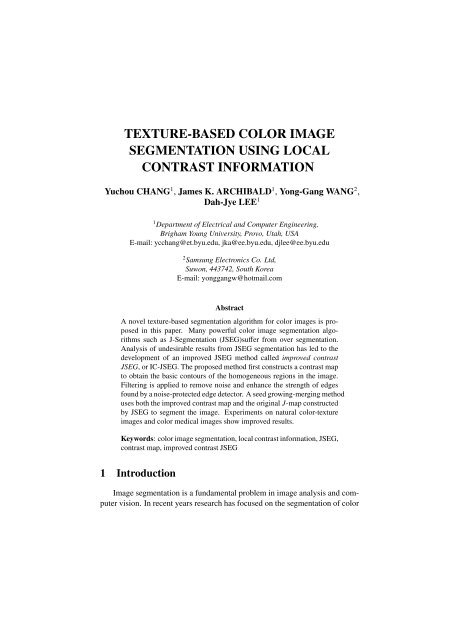
TEXTURE-BASED COLOR IMAGE<br />
SEGMENTATION USING LOCAL<br />
CONTRAST INFORMATION<br />
Yuchou CHANG 1 , James K. ARCHIBALD 1 , Yong-Gang WANG 2 ,<br />
Dah-Jye LEE 1<br />
1 Department of Electrical and Computer Engineering,<br />
Brigham Young University, Provo, Utah, USA<br />
E-mail: ycchang@et.byu.edu, jka@ee.byu.edu, djlee@ee.byu.edu<br />
2 Samsung Electronics Co. Ltd,<br />
Suwon, 443742, South Korea<br />
E-mail: yonggangw@hotmail.com<br />
Abstract<br />
A novel <strong>texture</strong>-<strong>based</strong> <strong>segmentation</strong> algorithm for <strong>color</strong> <strong>image</strong>s is proposed<br />
in this paper. Many powerful <strong>color</strong> <strong>image</strong> <strong>segmentation</strong> algorithms<br />
such as J-Segmentation (JSEG)suffer from over <strong>segmentation</strong>.<br />
Analysis of undesirable results from JSEG <strong>segmentation</strong> has led to the<br />
development of an improved JSEG method called improved <strong>contrast</strong><br />
JSEG, or IC-JSEG. The proposed method first constructs a <strong>contrast</strong> map<br />
to obtain the basic contours of the homogeneous regions in the <strong>image</strong>.<br />
Filtering is applied to remove noise and enhance the strength of edges<br />
found by a noise-protected edge detector. A seed growing-merging method<br />
uses both the improved <strong>contrast</strong> map and the original J-map constructed<br />
by JSEG to segment the <strong>image</strong>. Experiments on natural <strong>color</strong>-<strong>texture</strong><br />
<strong>image</strong>s and <strong>color</strong> medical <strong>image</strong>s show improved results.<br />
Keywords: <strong>color</strong> <strong>image</strong> <strong>segmentation</strong>, <strong>local</strong> <strong>contrast</strong> information, JSEG,<br />
<strong>contrast</strong> map, improved <strong>contrast</strong> JSEG<br />
1 Introduction<br />
Image <strong>segmentation</strong> is a fundamental problem in <strong>image</strong> analysis and computer<br />
vision. In recent years research has focused on the <strong>segmentation</strong> of <strong>color</strong>
<strong>image</strong>s, since grayscale <strong>image</strong>s can not satisfy the needs in many application<br />
domains. Color <strong>image</strong> <strong>segmentation</strong> divides a <strong>color</strong> <strong>image</strong> into a set of disjointed<br />
regions which are homogeneous with respect to some properties consistent<br />
with human visual perception, such as <strong>color</strong>s or <strong>texture</strong>s.<br />
In this paper, we consider the problem of natural <strong>image</strong> <strong>segmentation</strong> <strong>based</strong><br />
on <strong>color</strong> and <strong>texture</strong> information. Many <strong>texture</strong> or <strong>segmentation</strong> methods have<br />
been proposed in the literature, including [1] [3] [4] [8] [9] [10] [11] [15].<br />
Most of these are <strong>based</strong> on two basic properties of the pixels in relation to<br />
their <strong>local</strong> neighborhoods: discontinuity and similarity. Approaches <strong>based</strong> on<br />
discontinuity partition an <strong>image</strong> by detecting isolated points, lines, and edges.<br />
These are known as edge detection techniques. Similarity-<strong>based</strong> approaches<br />
group similar pixels into different homogenous regions; common methods include<br />
region growing, region splitting, region merging. More recently, new<br />
algorithms have been proposed that improve the accuracy of <strong>segmentation</strong> by<br />
integrating region and boundary information [7] [6] [16].<br />
Image <strong>texture</strong>, by definition, refers to the variation of <strong>color</strong> patterns within<br />
the <strong>image</strong>. Image regions with high levels of <strong>texture</strong> are typically nonhomogenous.<br />
For this reason, it is difficult to rely entirely on <strong>color</strong> discrimination to<br />
identify both homogeneous regions and the boundaries or edges between those<br />
regions. In [5], the JSEG method is proposed for the unsupervised <strong>segmentation</strong><br />
of <strong>color</strong> <strong>image</strong>s. In JSEG, <strong>color</strong>s are first quantized and then <strong>image</strong>s are<br />
spatially segmented. In practice, the boundary detection used by JSEG often<br />
produces results that exhibit over-<strong>segmentation</strong>, in which homogenous regions<br />
are unnecessarily and undesirably split into smaller subregions.<br />
In [2], a <strong>contrast</strong>-<strong>based</strong> <strong>color</strong> <strong>image</strong> <strong>segmentation</strong> method is proposed.<br />
Based on the subjective observations of ten participants, the authors concluded<br />
that perceived <strong>color</strong> <strong>contrast</strong> is weakly correlated with luminance and <strong>color</strong><br />
levels, as encoded in the CIE L ∗ a ∗ b ∗ <strong>color</strong> space. Although their <strong>segmentation</strong><br />
results are better than those of the original JSEG method with respect to over<strong>segmentation</strong>,<br />
the algorithm does not consider <strong>image</strong>s with complex <strong>texture</strong>s.<br />
Because the algorithm uses a single threshold for <strong>contrast</strong>, it often merges different<br />
regions – themselves each homogenous – into a single region, resulting<br />
in under-<strong>segmentation</strong>.<br />
In this paper, we propose a new algorithm <strong>based</strong> on JSEG for the <strong>segmentation</strong><br />
of <strong>color</strong> <strong>image</strong>s. Key to the new approach is a more effective measure<br />
of region homogeneity. Section 2 reviews the homogeneity measure defined<br />
by JSEG and discusses why it causes over-<strong>segmentation</strong>. Section 3 describes<br />
the new <strong>contrast</strong> map-<strong>based</strong> measure of homogeneity, and Section 4 presents<br />
experimental results that demonstrate the superiority of the new algorithm. Fi-<br />
2
nally, we offer conclusions in Section 5.<br />
2 JSEG Method<br />
The JSEG <strong>segmentation</strong> algorithm begins by reducing the <strong>color</strong>s in the<br />
<strong>image</strong> through quantization <strong>based</strong> on peer group filtering (PGF) and vector<br />
quantization. The result of <strong>color</strong> quantization is a class-map which logically<br />
associates the label of a <strong>color</strong> class with each pixel belonging to the class. The<br />
spatial <strong>segmentation</strong> that follows as the second step in JSEG is <strong>based</strong> on the<br />
information in the class-map. The following notation and discussion are <strong>based</strong><br />
on [5].<br />
Let Z be the set of all (x, y) <strong>image</strong> pixels contained in a particular classmap.<br />
Suppose that Z has been classified into C classes, Zi, i = 1, . . . , C. Define<br />
m to be the spatial mean of all points in Z, and denote the spatial mean of pixels<br />
in Zi as mi. The total variance of all points in Z is given by<br />
<br />
S T = z − m 2 . (1)<br />
z∈Z<br />
We can compute the total variance of points belonging to the same class as<br />
S W =<br />
C <br />
z − mi 2 . (2)<br />
i=1 z∈Zi<br />
A measure of the distribution of <strong>color</strong> classes is then given by<br />
J = (S T − S W)<br />
. (3)<br />
S W<br />
The JSEG algorithm continues by computing, for each pixel, a J value<br />
over a small window centered at that pixel. This results in a J-<strong>image</strong> or J-map<br />
with corresponding pixel values defined by <strong>local</strong> J values. The J-<strong>image</strong>s constructed<br />
at different scales specify <strong>local</strong> homogeneities, which in turn indicate<br />
potential boundary locations. The higher the <strong>local</strong> J value is, the more likely<br />
that the associated pixel is close to a region boundary.<br />
In [5], J values are calculated over the class-map so that <strong>color</strong> or intensity<br />
information of the original pixels is not considered. Fig. 1 shows two simple<br />
class-maps with similarly shaped regions. In this example, the labels “1”, “2”<br />
and “3” correspond to different classifications of data points. As can be seen,<br />
the intensity value of Class 3 is much higher than that of Class 2, while Class<br />
2’s intensity value is just slightly higher than that of Class 1. Despite the<br />
3
intensity differences, Equations (1)-(3) produce identical J values (0.6) for<br />
both two class-maps. Perceptually, the edge between Class 2 and Class 3 is<br />
sharper and has higher <strong>contrast</strong> than the edge between Classes 1 and 2. This<br />
example shows that the J measure can be used to detect boundaries, but the<br />
measure does not reflect the boundary strength. This illustrates one cause of<br />
over-<strong>segmentation</strong> in JSEG results.<br />
Figure 1. Two similar class-maps calculated with a 5×5 window size. Labels indicate<br />
pixel classification in Class 1, 2, or 3.<br />
3 Improved Contrast JSEG<br />
3.1 Contrast Map Construction<br />
We propose a new <strong>color</strong> <strong>image</strong> <strong>segmentation</strong> approach that addresses the<br />
limitations of the JSEG method. Our approach is <strong>based</strong> on the conclusion in [2]<br />
that <strong>color</strong> <strong>contrast</strong> is weakly correlated with luminance and <strong>color</strong> levels. We<br />
assume that the original <strong>image</strong> has first been converted to the CIE L∗a∗b∗ <strong>color</strong><br />
space. For two <strong>color</strong>s representations within that <strong>color</strong> space, c1 = (L∗ 1a∗ 1b∗ 1 )<br />
and c2 = (L∗ 2a∗ 2b∗ 2 ), the Euclidean distance between c1 and c2 is defined by<br />
∆Ec2c1 =<br />
<br />
(L ∗ 2 − L∗ 1 )2 + (a ∗ 2 − a∗ 1 )2 + (b ∗ 2 − b∗ 1 )2 . (4)<br />
This measure of distance approximates the perceptual difference between two<br />
<strong>color</strong>s [14].<br />
For pixel p(i, j) in <strong>image</strong> I(i, j), the <strong>contrast</strong> can be calculated from the 3×3<br />
surrounding window <strong>using</strong> the Euclidean distance in CIE L ∗ a ∗ b ∗ <strong>color</strong> space<br />
4
as<br />
<strong>contrast</strong>(i, j) = MAX <br />
∆Ep(i+m, j+n)p(i, j) − MIN ∆Ep(i+m, j+n)p(i, j) ,<br />
m ∈ {−1, 0, 1}, n ∈ {−1, 0, 1} (5)<br />
However, the <strong>contrast</strong> map constructed <strong>using</strong> values obtained from Equation<br />
(5) is usually noisy, and the noise negatively affects the final <strong>segmentation</strong><br />
result.<br />
3.2 Improved Contrast Map (ICMap<br />
Our approach improves the <strong>contrast</strong> map by reducing the noise and enhancing<br />
the boundary strength <strong>using</strong> a filter proposed in [13]. Based on a<br />
256-grayscale <strong>contrast</strong> map, quantized from <strong>contrast</strong>(i, j), a two-step procedure<br />
is applied to the <strong>image</strong> channels in order to increase the effectiveness of<br />
the smoothing operation. The first step of this procedure is defined by the<br />
following equations.<br />
c (1) (i, j) = c (0) (i, j) + 1<br />
8<br />
c (2) (i, j) = c (1) (i, j) + 1<br />
8<br />
1<br />
1<br />
m=−1 n=−1,<br />
(m,n)(0,0)<br />
1<br />
1<br />
m=−1 n=−1,<br />
(m,n)(0,0)<br />
ς (1) (c (0) (i + m, j + n), c (0) (i, j)) (6)<br />
ς (2) (c (1) (i + m, j + n), c (1) (i, j)) (7)<br />
where ς (p) is the parameterized nonlinear function given by<br />
ς (p) ⎧<br />
u − v<br />
⎪⎨<br />
(u, v) =<br />
⎪⎩<br />
: |u − v| ≤ a (p)<br />
<br />
3a (p) − u + v<br />
sgm(u − v)<br />
2<br />
: a (p) < |u − v| ≤ 3a (p)<br />
0 : |u − v| > 3a (p)<br />
and a (p) is an integer such that 0 < a (p) < L. (In this case L = 256.) In the<br />
filter, small a (p) values preserve the fine details, and large values produce a<br />
strong noise cancellation [12].<br />
The second step of Russo’s filter [13] takes into account the differences<br />
between the pixel to be processed and its neighboring pixels in a slightly different<br />
way: if all these differences are very large, the pixel is (possibly) part of<br />
5<br />
(8)
a boundary that may be considered noise and may be cancelled. (Real boundaries<br />
will be enhanced in a future step.) This step is briefly summarized as<br />
follows.<br />
where<br />
c (3) (i, j) = c (2) (i, j) − (L − 1)∆(i, j) (9)<br />
∆(i, j) = MIN µLA(c (2) (i, j), c (2) (i + m, j + 2)) −<br />
MIN µLA(c (2) (i + m, j + n), c (2) (i, j)) ,<br />
m ∈ {−1, 0, 1}, n ∈ {−1, 0, 1}, (m, n) (0, 0) (10)<br />
and µLA(u, v) denotes the membership function that describes the fuzzy relation<br />
“u is much larger than v”:<br />
⎧ u − v<br />
⎪⎨ : 0 < u − v ≤ L − 1<br />
µLA(u, v) = L − 1<br />
(11)<br />
⎪⎩ 0 : u − v ≤ 0<br />
To enhance the boundaries after <strong>image</strong> filtering, the output of the <strong>color</strong><br />
edge detector is given by<br />
ICMap(i, j) = (L − 1) (1 − MIN {µSM(B1), µSM(B2)}) (12)<br />
where µSM is the membership function for another fuzzy set, and B1 and B2<br />
are Euclidean distances between averages of selected <strong>color</strong> vectors. (See [13]<br />
for a detailed explanation.)<br />
This improved <strong>contrast</strong> map (ICMap) reduces noise and enhances the boundaries<br />
to a large extent.<br />
3.3 A Novel Measure Definition and Spatial Segmentation<br />
A new measure combining the ICMap and J measure in JSEG can be constructed<br />
for <strong>color</strong> <strong>texture</strong>-<strong>based</strong> <strong>segmentation</strong>. The proposed new method is<br />
called IC-JSEG. For an M×N <strong>image</strong>, ICMap is first calculated according to<br />
Equation (5), and then improved according to Equation (12). At this point, the<br />
magnitude is normalized as follows:<br />
where<br />
wIC(i, j) =<br />
ICMap(i, j)<br />
ICMap max<br />
(13)<br />
ICMap max = MAX {ICMap(i, j)} , 0 ≤ i ≤ M − 1, 0 ≤ j ≤ N − 1. (14)<br />
6
The J value (also normalized) of the <strong>local</strong> region is computed according to<br />
Equations (1)-(3). Then the proposed measure is formed by weighting the J as<br />
follows: WIC.<br />
JIC(i, j) = wIC(i, j) · J(i, j). (15)<br />
With the integration of ICMap, the J map can be strengthened to distinguish<br />
the edges from inner details.<br />
Using the new JIC measure, we construct a JIC <strong>image</strong> or map, where pixel<br />
values can be used to indicate the interior and boundary of the region. We<br />
also adopt the multi-scale <strong>segmentation</strong> scheme provided by JSEG, consisting<br />
of three main operations: seed area determination, region growing, and<br />
region merging. Starting at a coarse initial scale, the following processes are<br />
performed repetitively in a multi-scale manner until all the pixels are classified.<br />
1. Seed area determination. A set of initial seed areas is determined to be<br />
the basis for region growing. First, a threshold is set to find the seed<br />
areas: T = µ + δσ, where µ and σ are the average and the standard<br />
deviation of the <strong>local</strong> JIC values in the regions, respectively, and δ is<br />
a constant. Then pixels with JIC values less than T are connected and<br />
considered as a seed.<br />
2. Seed growing. The new regions are grown from the seed regions selected<br />
in Step 1. First, the the <strong>local</strong> JIC values in the remaining unsegmented<br />
part of the regions are averaged. Then, pixels with values below that<br />
average are assigned to an adjacent seed. For the remaining pixels, their<br />
<strong>local</strong> JIC values are calculated. They will be dealt with at the next finer<br />
scale to more accurately locate the boundaries.<br />
Region growing is followed by a region merging operation to give the final<br />
segmented <strong>image</strong>. The <strong>color</strong> histogram for each region is extracted, where<br />
the quantized <strong>color</strong>s from the <strong>color</strong> quantization process are used as the <strong>color</strong><br />
histogram bins. The two regions with the minimum distance between their<br />
histograms are merged together and this process continues until a maximum<br />
distance threshold is reached.<br />
Fig. 2(a) illustrates the effects of applying the new IC-JSEG algorithm to<br />
the “Garden” <strong>image</strong>. Image (a) in the figure shows the original <strong>image</strong>, and<br />
(b) and (c) show the J map and <strong>contrast</strong> map from the original JSEG method,<br />
respectively. Figs. 2(d) and (e) represent the improved <strong>contrast</strong> map and J<br />
map <strong>using</strong> the IC-JSEG algorithm. Figs. 2(f) and (g) show the final segmented<br />
<strong>image</strong>s <strong>using</strong> JSEG and IC-JSEG respectively.<br />
7
(a) (b) (c)<br />
(d) (e)<br />
(f) (g)<br />
Figure 2. (a) Original <strong>image</strong> (b) J map (c) Contrast map (d) ICMap (e) JIC map (f)<br />
JSEG <strong>segmentation</strong> result (g) Result from proposed <strong>segmentation</strong> method<br />
4 Experimental Results<br />
The proposed algorithm was applied to a set of natural <strong>color</strong> <strong>image</strong>s with<br />
varying <strong>texture</strong>s and to a set of medical <strong>image</strong>s, and the results were compared<br />
with <strong>segmentation</strong> results of the original JSEG algorithm. To test the overall<br />
robustness of the algorithm, our experiments did not include any fine-tuning<br />
of parameters for individual <strong>image</strong>s. Parameters common to both JSEG and<br />
IC-JSEG were set to identical values for the experiments shown. Fig. 3 shows<br />
the <strong>segmentation</strong> results obtained by the JSEG and IC-JSEG methods.<br />
From Fig. 3, we can see that the results obtained from the proposed IC-<br />
JSEG method are better than those obtained <strong>using</strong> the original JSEG method.<br />
With JSEG, the lawn and trees are split apart into many small regions. In<br />
<strong>contrast</strong>, IC-JSEG keeps them as an integral part which more closely matches<br />
human visual perception. Furthermore, for the mountain, lake, buildings, and<br />
8
(a) (b) (c)<br />
Figure 3. (a) Original natural <strong>color</strong>-<strong>texture</strong> <strong>image</strong>s, (b) Results of JSEG method, (c)<br />
Results of the proposed method.<br />
9
so forth, IC-JSEG preserves more homogeneous regions than does JSEG.<br />
The new IC-JSEG method was also applied to three <strong>color</strong> medical <strong>image</strong>s<br />
to test its performance, as shown in Fig. 4. From the results of these <strong>color</strong>ed<br />
cell <strong>image</strong>s, we can see that IC-JSEG detects more homogeneous regions<br />
than the JSEG method does. Since the IC-JSEG method strengthens edges to<br />
discriminate different homogeneous regions, it can also detect trivial homogeneous<br />
regions. Although IC-JSEG segments the <strong>image</strong>s into more regions,<br />
these segmented regions conform more closely to human visual perception,<br />
and they are not considered to be evidence of over-<strong>segmentation</strong>.<br />
(a) (b) (c)<br />
Figure 4. (a) Original natural <strong>color</strong>-<strong>texture</strong> <strong>image</strong>s, (b) Results of JSEG method, (c)<br />
Results of the proposed method.<br />
5 Conclusion<br />
Color and <strong>texture</strong> are critical factors in human visual perception. Many<br />
<strong>segmentation</strong> approaches use both factors to obtain homogeneous regions for<br />
10
<strong>segmentation</strong>. In this paper, a new measure of homogeneity is proposed for<br />
<strong>segmentation</strong> <strong>based</strong> on <strong>color</strong> <strong>texture</strong>. The measure integrates textural homogeneity<br />
and edge information to overcome the drawbacks of the JSEG method<br />
on which our overall algorithm is <strong>based</strong>. After analyzing the over-<strong>segmentation</strong><br />
problem of the JSEG method, we proposed the use of <strong>contrast</strong> visual information<br />
to form a <strong>contrast</strong> map. We adopted noise removal and edge enhancement<br />
strategies to construct an improved <strong>contrast</strong> map to form explicit outlines of<br />
major objects in the <strong>image</strong>. Next, the improved <strong>contrast</strong> map (ICMap) and<br />
original J-map are combined to form a new JIC map. Based on the new JIC<br />
map we use a seed growing-merging method to segment the <strong>image</strong>. Experiments<br />
performed on both natural and medical <strong>image</strong>s show that the proposed<br />
method is robust for both and produces segmented <strong>image</strong>s that better match<br />
human perception than the original JSEG method.<br />
Acknowledgments<br />
The authors extend thanks ro our colleague Hong-Xing Qin at Shanghai<br />
Jiaotong University for sharing the <strong>color</strong> medical <strong>image</strong>s.<br />
References<br />
[1] Chang, T., Kuo, C.-C.J. 1993, Texture analysis and classification with<br />
tree-structured wavelet transform, IEEE Transactions on Image Processing,<br />
Vol. 2, No. 4, pp. 429-441.<br />
[2] Chen, H.C., Chien. W.J., Wang S.J., 2004, Contrast-<strong>based</strong> <strong>color</strong> <strong>image</strong><br />
<strong>segmentation</strong>, IEEE Signal Processing Letters, Vol. 11, No. 7, pp. 641-<br />
644.<br />
[3] Comaniciu, D., Meer, P., 1997, Robust analysis of feature spaces: <strong>color</strong><br />
<strong>image</strong> <strong>segmentation</strong>, IEEE Int. Conf. on Computer Vision and Pattern<br />
Recognition, San Juan, Puerto Rico, pp. 750-755.<br />
[4] Comaniciu, D., Meer, P., 2002, Mean shift: a robust approach toward<br />
feature space analysis, IEEE Transactions on Pattern Analysis and Machine<br />
Intelligence, Vol. 24, No. 5, pp. 603-619.<br />
[5] Deng, Y., Manjunath, B.S., 2001, Unsupervised <strong>segmentation</strong> of <strong>color</strong><strong>texture</strong><br />
regions in <strong>image</strong>s and video, IEEE Transactions on Pattern Analysis<br />
and Machine Intelligence, Vol. 23, No. 8, pp. 800-810.<br />
11
[6] Fan, J., Yau, D.K.Y., Elmagarmid, A.K., Aref, W.G., 2001, Automatic<br />
<strong>image</strong> <strong>segmentation</strong> by integrating <strong>color</strong>-edge extraction and seeded region<br />
growing, IEEE Transactions on Image Processing, Vol. 10, No. 10,<br />
pp. 1454-1466.<br />
[7] Freixenet, J., Muñoz, X., Raba, D., Marti, J., Cufi, X., 2002, Yet another<br />
survey on <strong>image</strong> <strong>segmentation</strong>: region and boundary information integration,<br />
Proc. 7th European Conference on Computer Vision – Part III,<br />
Copenhagen, Denmark, pp. 408-422.<br />
[8] Luo, J., Gray, R.T., Lee, H.C., 1998, Incorporation of derivative priors<br />
in adaptive Bayesian <strong>color</strong> <strong>image</strong> <strong>segmentation</strong>, IEEE Int. Conf. on<br />
Image Processing, Chicago, IL, pp. 780-784.<br />
[9] Luo, Q., Khoshgoftaar, T.M., 2006, Unsupervised multiscale <strong>color</strong> <strong>image</strong><br />
<strong>segmentation</strong> <strong>based</strong> on MDL principle, IEEE Transactions on Image<br />
Processing, Vol. 15, No. 9, pp. 2755-2761.<br />
[10] Pappas, T.N., 1992, An adaptive clustering algorithm for <strong>image</strong> <strong>segmentation</strong>,<br />
IEEE Transactions on Signal Processing, Vol. 40, No. 4, pp. 901-<br />
914.<br />
[11] Randen, T., Husoy, J.H. 1999, Texture <strong>segmentation</strong> <strong>using</strong> filters with<br />
optimized energy separation, IEEE Transactions on Image Processing,<br />
Vol. 8, No. 4, pp. 571-582.<br />
[12] Russo, F., 2003, A method for estimation and filtering of Gaussian noise<br />
in <strong>image</strong>s, IEEE Transactions on Instrumentation and Measurement, Vol.<br />
52, No. 4, pp. 1148-1154.<br />
[13] Russo, F., Lazzari, A., 2005, Color edge detection in presence of Gaussian<br />
noise <strong>using</strong> nonlinear prefiltering, IEEE Transactions on Instrumentation<br />
and Measurement, Vol. 54, No. 1, pp. 352-358.<br />
[14] Ruzon M.A., Tomasi, C., 2001, Edge, junction, and corner detection<br />
<strong>using</strong> <strong>color</strong> distributions, IEEE Transactions on Pattern Analysis and<br />
Machine Intelligence, Vol. 23, No. 11, pp. 1281-1295.<br />
[15] Unser, M., 1995, Texture classification and <strong>segmentation</strong> <strong>using</strong> wavelet<br />
frames, IEEE Transactions on Image Processing, Vol. 4, No. 11, pp.<br />
1549-1560.<br />
[16] Xu, J., Shi, P.F., 2003, Natural <strong>color</strong> <strong>image</strong> <strong>segmentation</strong>, Proc. IEEE<br />
Int. Conf. Image Processing, Vol. 1, Barcelona, Spain, pp. 973-976.<br />
12