JRA2 Progress report on IR multispectral imaging - Eu-ARTECH

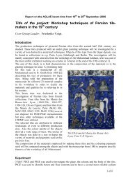
THIRD ANNUAL REPORT - DELIVERABLE N. 27
<strong>JRA2</strong> – New methods in diagnostics: Imaging and
spectroscopy
<strong>Progress</strong> <strong>report</strong> on IR multispectral imaging - IR
transparency and system assembling
Eu-ARTECH
Access, Research and Technology for the conservation
of the European Cultural Heritage
Integrating Activity
implemented as
Integrated Infrastructure Initiative
Contract number: RII3-CT-2004-506171
Project Co-ordinator: Prof. Brunetto Giovanni Brunetti
Reporting period: from June 1 st 2005 to May 31 st 2006
Project funded by the European Community
under the “Structuring the European Research Area”
Specific ProgrammeResearch Infrastructures action
1

DELIVERABLE n.27
<strong>JRA2</strong>- <strong>Progress</strong> <strong>report</strong> on IR multispectral imaging - IR transparency and system
assembling
Subtask 2.3- Assembling of nIR imaging equipments - Development of two new
complementary NIR imaging spectroscopy methods.
Subtask 2.4 Evaluation of the device
Resp. : OADC
During this <strong>report</strong>ing period, the set-up of the prototypical form of the spectrograph (already
developed and described in the previous <strong>report</strong>s) continued with adjustments of the
alignments of the various optical components. The performances were improved.
The measurements on the various samples, already developed in the previous periods, also
continued.
In Appendix 2 of the present Annex 14, are <strong>report</strong>ed most of the spectra that have been
recorded during the last six months.
Subtask 2.1 - Preparation and characterisation of standards of layered painting materials
and Subtask 2.2- Transmission and reflection of IR radiation on layered standards
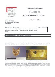
Within the period between the 12 th and the 24 th month special reference samples were
developed on wooden panels of gradually higher paint layer thickness in order to
study the transmission and reflection of the IR radiation through them. The way that
these reference samples are created is displayed in figure 1.1a. Multi-spectral spectra
of these samples will be acquired in the visible, near infrared (nIR) and mid infrared
(mIR) area of the spectrum (up to 4500nm).
Figure 1.1a: Reference sample (way of fabrication of gradually higher thickness )
The reference samples are painted on a common white ground and with the same binding medium in
order to minimize the uncertainty to our applied algorithms during the tests.
Ground : CaCO3 + animal glue
Binding Medium : Egg yolk
In appendix 1 all the first testing measurements on the panels are provided. For the
time being the Perkin ELMER lambda 900 spectrophotometer was used in the
wavelength range of 200nm-2400nm. These measurements will serve as a reference
2

for the testing of the device under development. Within the next months and after the
first assembly of the device, the measurements will be performed using the new device
and the new developed method will be tested in the extensive wavelength range
between 800nm and 4500nm.
Materials and methodology of creation of the reference panels (standards)
Samples of pigments in paint layers of gradually higher thickness.
The panels with samples of different (gradually higher) thickness were prepared in successive
steps, as follows: first, all eight parts of one pigment sample were painted at once in 2 or 3
layers of paint, then one part was masked out and the remaining seven layers were painted
again in 2 or 3 layers. Then two parts were masked and the remaining six were painted, and so
forth. Between each step, the paint was allowed to dry satisfactorily. The panels were setaside
for a month to dry well before the first measurements are taken.
The panels for the samples of different thickness were prepared by lightly scoring rectangles,
separated in 8 parts each of 2x5cm. These were then split in two lengthwise, one half painted
in 3 layers of carbon black with egg as a binding medium and the other scored in pencil with
diagonal lines, again on half of its area.
Figure 1.1.2a: Samples of 10 pigments in paint layers of gradually higher thickness.
3

Subtask 2.3: Assembling of nIR spectroscopic imaging equipment
Description of the overall developed system
The system will be capable of acquiring spectra in diffuse reflectance mode from
800nm up to 4500nm. This is a wavelength area that is not examined extensively up
to now in the field of artworks materials identification using IR radiation (imaging or
spectroscopy in diffuse reflectance mode).
The aim is the generation of mapping images of a Region Of Interest (ROI) or the
whole painting as far as the materials distribution is concerned. The UV –Vis -nIR
spectral area is extensively examined. Using the device that will be assembled, the
spectral area of examination will extended up to 4500nm. The basic idea of the
interferometer that is widely used in the available FTIR systems will be used in order
to send monochromatic radiation to the measurement point. The range of the
excitation system is 680nm up to 4800nm. The overall diagram of the system is
provided in fig. 1.2.1a
Figure 1.2.1a: overall diagram of the system
The radiation is produced in the spectrometer using the source and the interferometer
and the beam splitter. Then the beam is inserted in the fiber optic bundle. After the
fiber optic bundle the beam is condensed to the measurement area using the lens
system installed on the external integration sphere (fig. 1.2.1.3d). The diffuse
4

eflected light is collected to the detector which is also installed on the integration
shpere (fig. 1.2.1.4a)
The basic characteristics of the assembled device are provided in table 3.2.2a
Table 3.2.2a:
Parameter Value
1. Wavelength range :
800-4500 nm
2. Measurement Spot Size: 2-4 mm diameter depending on
the wavelength range
3. Time of measurement (spectra 4-10 sec
acquisition in all the wavelength range)
4. Wavelength resolution 0,1-6,4 nm (variable)
5. Parts to be assembled (brochures with
technical specs)
5.1. MCT HgCdTe detector TE 800-4500nm
cooled (Not Liquid Nitrogen)
5.2 Matched Pre-Amplifiers
5.3 Fiber optics 650nm to 5000 nm
Heavy Metal Fluoride glass
fibers (SG TM fiber)
5.4 Integration Sphere (diffuse
reflectance measurement)
6. Drivers of the system, libraries in
Visual Studio (C++ or Basic)
5
Remote gold integrating sphere
(for diffuse reflectance
measurement)
Will be developed with the
assembly of the system
Use of a standard interferometer for a basic spectrometer:
A basic NIR-mIR spectrometer; from the commercial spectrometer available either
the PE Spectrum One NTS or a Nicolet NIR or a Bruker spectrometer are the
preferred systems in terms of energy throughput; the MIR scanner from Oriel is very
limited in energy to meet the overall goals; The PE system is finally preferred for
price /performance reasons;
External Integration Sphere:
An external integration sphere is the much best approach as far as wl range and
signal/noise are concerned in order to provide the possibility to the user to perform in
situ measurements. The integration sphere is gold coated in order to reflect the
radiation within the wavelength range of 800nm up to 4500nm.
nIR-mIR fibers:
The solutions are:
1. gold coated lightpipes which are subject to low energy throughout and very high
senistivity to mechanical movement,
2. chalcogenide (CaF2) fibers are critical in mechanical movement and tend to break,
transmission characteristics. They are superior to gold coated light pipes,

3. heavy metal fluorides (e.g. Zr) seem to be the most promising solution, as they are
mechanically stable with high energy throuput, price may be a criterium;
Detector:
The possibilities compatible with he solution of the PE spectrometer were: 1. DTGS
and MCT:
The MCT detector shows about a 100 fold higher sensitivity than the standard DTGS
detector; they are available with Peltier thermostatting without liquid nitrogen
coutercooling at a justifiable price.
Part of the used spectrophotometer
The interferometer and the beam splitter of the Perkin Elmer Spectrum One NTS is
used in order to produce the radiation which radiates the object (fig. 1.2.1.1).
Figure 1.2.1.1: The interferometer and the beam splitter of PE Spectrum One NTS
that is used.
6

Fiber optic bundle
The IR fiber bundle optic that is used has an attenuation curve provided in figure
1.2.1.2. The material of the fiber optic is finally heavy metal Zr fluoride.
Figure 1.2.1.2: Attenuation curve of the fiber optic that is used for the
nIR-mIR multispectral mapping imaging device.
Integration sphere design and assembly
The probe for in situ measurement is assembled using an integration sphere of
gold surface in order to have the possibility to integrate the radiation in the
specified wavelengths up to 4500nm. The spot size of the probe is a circle
with a diameter of 2mm approximately. This is changing while the excitation
wavelength is changing. The final spot size in relation with the wavelength is
subjected to further study.
The design of the integration sphere is displayed in Fig 1.2.1.3a-b and the final
developed sphere in fig. 1.2.1.3c
Figure 1.2.1.3a: Integration sphere that s developed and used for diffused
reflectance measurements from 800nm up to 4500nm the dimensions are in
INCHES.
7

Condensing lens
Figure 1.2.1.3b: Integration sphere that is developed and used for diffused
reflectance measurements from 800nm up to 4500nm the dimensions are in
INCHES.
Figure 1.2.1.3c: Integration sphere that will be used for diffused reflectance
measurements from 800nm up to 4500nm.
Detector
The diffused reflected radiation from the measuring area will be guided to the
receiving detector which is an (HgCdTe) Mercury Cadmium Telluride (MCT)
detector (800nm – 4500nm) mounted on a 3-stage cooler, in a TO-3 housing
on the integration sphere (fig. 1.2.1.4a). In figure 1.2.1.4b and c the MCT
sensors technical information is provided (The way that the sensor is
constructed (b) and the electronic circuit used to calculate the amplifiers that
will be used for the amplification of the received signal (c)). The detectivity
curve of the sensor is provided in figure 1.2.1.4c (MCT-5-TE).
8
collimating lens

9
MCT-Detector
Figure 1.2.1.4a: The detector and the way that is mounted on the integration
sphere
Figure 1.2.1.4b: The detector (way that the
detector is constructed
Figure 1.2.1.4b: the electronic circuit used
to calculate the matched amplifiers that will
be used for the amplification of the received
signal)
Figure 1.2.1.4c: The detector sensitivity curve (800nm – 4500nm)

The sensor is interconnected with the suitable electronic pre-amplifier because
the sufficiency of the received power is critical (figure 1.2.1.4d).
Figure 1.2.1.4d: preamplifier for the detector
Initial evaluation of the system
Measurements were acquired from the already developed reference samples in order
to justify the penetration of the radiation to the paint layers of the artworks. The
measurements were applied to the reference panel with the pigments that are painted
with gradually increasing thickness (fig. 1.1.2a). The spectra that are acquired with
the developed device are the same with the previous spectra acquired with the Perkin
Elmer lambda 900 (provided in Appendix 1) in the overlapping area 800-2500nm.
This fact ensures that the device works efficiently.
The radiation penetrates even the thickest layers since the spectra have lower
reflectivity over the white background while the thickness increases. In the case of the
black background the reflectivity increases while the thickness of the layer increase.
These measurements are shown in appendix 2. A golden sample is also measured in
order to validate the operation of the system. The result is shown in fig. 1.2.1.5. As
expected the gold has a reflectivity of almost 100% in the specific wavelength area
(800nm-4500nm).
In the NIR spectral region (800-2500 nm) overtone and combination vibrational
modes are active, whereas in the 2500-4200 nm region some fundamental vibrations
can be observed. Almost all the absorption bands observed in the NIR arise from
overtones of functional groups containing hydrogen atoms (C-H, N-H, O-H) or
combinations involving stretching and bending modes of vibration of such groups. A
great degree of complexity characterizes the spectra acquired in this region. As a
result, spectral assignments to specific vibrational modes are not always possible.
10

Figure 1.2.1.5 Gold sample measurement (90% reflectivity)
(800nm – 4500nm)
11

APPENDIX 1
Vertical axis (Reflectivity R%) - Horizontal axis Wavelengths (200-2400nm)
Lead White
(over Black)
100
90
80
70
60
50
40
30
20
10
0
0 500 1000 1500 2000 2500
Yellow Ochre
(over Black)
60
50
40
30
20
10
0
0 500 1000 1500 2000 2500
Warm Ochre
(over Black)
50
45
40
35
30
25
20
15
10
5
0
0 500 1000 1500 2000 2500
12
(over White)
90
80
70
60
50
40
30
20
10
0 500 1000 1500 2000 2500
(over White)
70
60
50
40
30
20
10
0
0 500 1000 1500 2000 2500
80
70
60
50
40
30
20
10
(over White)
0
0 500 1000 1500 2000 2500

Red Ochre
(over Black)
35
30
25
20
15
10
5
0
0 500 1000 1500 2000 2500
Sienna Burnt
(over Black)
30
25
20
15
10
5
0
0 500 1000 1500 2000 2500
Hematite
(over Black)
40
35
30
25
20
15
10
5
0
0 500 1000 1500 2000 2500
13
70
60
50
40
30
20
10
(over White)
0
0 500 1000 1500 2000 2500
(over White)
70
60
50
40
30
20
10
0
0 500 1000 1500 2000 2500
60
50
40
30
20
10
(over White)
0
0 500 1000 1500 2000 2500

Caput Mortuum
(over Black)
70
60
50
40
30
20
10
0
0 500 1000 1500 2000 2500
Umber Raw(over Black)
50
45
40
35
30
25
20
15
10
5
0
0 500 1000 1500 2000 2500
Cinnabar
(over Black)
70
60
50
40
30
20
10
0
0 500 1000 1500 2000 2500
14
0.8
0.7
0.6
0.5
0.4
0.3
0.2
0.1
(over White)
0
0 500 1000 1500 2000 2500
60
50
40
30
20
10
0
(over White)
-10
0 500 1000 1500 2000 2500
70
60
50
40
30
20
10
(over White)
0
0 500 1000 1500 2000 2500

Minium
(over Black)
90
80
70
60
50
40
30
20
10
0
0 500 1000 1500 2000 2500
Green Earth
(over Black)
30
25
20
15
10
5
0
-5
-10
-15
0 500 1000 1500 2000 2500
Malachite
(over Black)
40
30
20
10
0
-10
-20
0 500 1000 1500 2000 2500
15
0.35
0.3
0.25
0.2
0.15
0.1
0.05
-0.05
-0.1
140
120
100
0
80
60
40
20
(over White)
0
0 500 1000 1500 2000 2500
(over White)
-0.15
0 500 1000 1500 2000 2500
60
50
40
30
20
10
0
-10
(over White)
-20
0 500 1000 1500 2000 2500

Azzurite
(over Black)
40
35
30
25
20
15
10
5
0
0 500 1000 1500 2000 2500
Ultramarine
(over Black)
25
20
15
10
5
0
-5
-10
0 500 1000 1500 2000 2500
Indigo
(over Black)
25
20
15
10
5
0
-5
0 500 1000 1500 2000 2500
16
80
70
60
50
40
30
20
10
0
(over White)
-10
0 500 1000 1500 2000 2500
80
70
60
50
40
30
20
10
(over White)
0
0 500 1000 1500 2000 2500
100
90
80
70
60
50
40
30
20
10
(over White)
0
0 500 1000 1500 2000 2500

Cobalt Blue(over Black)
60
50
40
30
20
10
0
-10
0 500 1000 1500 2000 2500
17
(over White)
70
60
50
40
30
20
10
0
0 500 1000 1500 2000 2500

APPENDIX 2
Vertical axis (Reflectivity R%) - Horizontal axis Wavelengths (800-4500nm)
% Reflectance
30
25
20
15
10
5
0
800 1200 1600 2000 2400 2800 3200 3600 4000
% Reflectance
80
70
60
50
40
30
20
10
Wavelength nm
Azurite b1
Azurite b2
Azurite b3
Azurite b4
Azurite b5
Azurite b6
Azurite b7
Azurite b8
0
800 1200 1600 2000 2400 2800 3200 3600 4000
Wavelength nm
Azurite on black and white
Caput Mortuum on black and white
Caput Mortuum b1
Caput Mortuum b2
Caput Mortuum b3
Caput Mortuum b4
Caput Mortuum b5
Caput Mortuum b6
Caput Mortuum b7
Caput Mortuum b8
% Reflectance
100
90
80
70
60
50
40
30
20
10
% Reflectance
100
80
60
40
20
0
800 1200 1600 2000 2400 2800 3200 3600 4000
Wavelength nm
Azurite w1
Azurite w2
Azurite w3
Azurite w4
Azurite w5
Azurite w6
Azurite w7
Azurite w8
Caput Mortuum w1
Caput Mortuum w2
Caput Mortuum w3
Caput Mortuum w4
Caput Mortuum w5
Caput Mortuum w6
Caput Mortuum w7
Caput Mortuum w8
0
800 1200 1600 2000 2400 2800 3200 3600 4000
Wavelength nm
18

% Reflectance
100
90
80
70
60
50
40
30
20
10
0
800 1200 1600 2000 2400 2800 3200 3600 4000
% Reflectance
40
30
20
10
Wavelength nm
Cinnabar on black and white
Cinnabar b1
Cinnabar b2
Cinnabar b3
Cinnabar b4
Cinnabar b5
Cinnabar b6
Cinnabar b7
Cinnabar b8
0
800 1200 1600 2000 2400 2800 3200 3600 4000
Wavelength nm
% Reflectance
100
Green Earth on black and white
Green Earth b1
Green Earth b2
Green Earth b3
Green Earth b4
Green Earth b5
Green Earth b6
Green Earth b7
Green Earth b8
% Reflectance
60
50
40
30
20
10
90
80
70
60
50
40
30
20
10
Cinnabar w1
Cinnabar w2
Cinnabar w3
Cinnabar w4
Cinnabar w5
Cinnabar w6
Cinnabar w7
Cinnabar w8
0
800 1200 1600 2000 2400 2800 3200 3600 4000
Wavelength nm
Green Earth w1
Green Earth w2
Green Earth w3
Green Earth w4
Green Earth w5
Green Earth w6
Green Earth w7
Green Earth w8
0
800 1200 1600 2000 2400 2800 3200 3600 4000
Wavelength nm
19

Hematite on black and white
80
40
Hematite w1
Hematite w2
Hematite w3
Hematite w4
Hematite w5
Hematite w6
Hematite w7
Hematite w8
70
60
30
50
40
Hematite b1
Hematite b2
Hematite b3
Hematite b4
Hematite b5
Hematite b6
Hematite b7
Hematite b8
20
30
% Reflectance
% Reflectance
20
10
10
800 1200 1600 2000 2400 2800 3200 3600 4000
0
800 1200 1600 2000 2400 2800 3200 3600 4000
0
Wavelength nm
Wavelength nm
Indigo on black and white
10
100
90
Indigo w1
Indigo w2
Indigo w3
Indigo w4
Indigo w5
Indigo w6
Indigo w7
Indigo w8
80
8
70
60
Indigo b1
Indigo b2
Indigo b3
Indigo b4
Indigo b5
Indigo b6
Indigo b7
Indigo b8
6
50
40
% Reflectance
% Reflectance
30
4
20
10
0
800 1200 1600 2000 2400 2800 3200 3600 4000
Wavelength nm
800 1200 1600 2000 2400 2800 3200 3600 4000
2
Wavelength nm
20

% Reflectance
90
80
70
60
50
40
30
20
10
0
800 1200 1600 2000 2400 2800 3200 3600 4000
% Reflectance
50
40
30
20
10
Wavenumber nm
Lead White b1
Lead White b2
Lead White b3
Lead White b4
Lead White b5
Lead White b6
Lead White b7
Lead White b8
0
800 1200 1600 2000 2400 2800 3200 3600 4000
Wavelength nm
Lead White on black and white
% Reflectance
100
Malachite on black and white
Malachite b1
Malachite b2
Malachite b3
Malachite b4
Malachite b5
Malachite b6
Malachite b7
Malachite b8
% Reflectance
80
70
60
50
40
30
20
10
90
80
70
60
50
40
30
20
10
Lead White w1
Lead White w2
Lead White w3
Lead White w4
Lead White w5
Lead White w6
Lead White w7
Lead White w8
0
800 1200 1600 2000 2400 2800 3200 3600 4000
Wavenumber nm
Malachite w1
Malachite w2
Malachite w3
Malachite w4
Malachite w5
Malachite w6
Malachite w7
Malachite w8
0
800 1200 1600 2000 2400 2800 3200 3600 4000
Wavelength nm
21

% Reflectance
100
90
80
70
60
50
40
30
20
10
0
800 1200 1600 2000 2400 2800 3200 3600 4000
% Reflectance
40
35
30
25
20
15
10
5
Wavelength nm
Minium on black and white
Minium b1
Minium b2
Minium b3
Minium b4
Minium b5
Minium b6
Minium b7
Minium b8
0
800 1200 1600 2000 2400 2800 3200 3600 4000
Wavelength nm
% Reflectance
120
110
100
Red Ochre on black and white
Red Ochre b1
Red Ochre b2
Red Ochre b3
Red Ochre b4
Red Ochre b5
Red Ochre b6
Red Ochre b7
Red Ochre b8
% Reflectance
90
80
70
60
50
40
30
20
10
90
80
70
60
50
40
30
20
10
Minium w1
Minium w2
Minium w3
Minium w4
Minium w5
Minium w6
Minium w7
Minium w8
0
800 1200 1600 2000 2400 2800 3200 3600 4000
Wavelength nm
0
800 1200 1600 2000 2400 2800 3200 3600 4000
Wavelength nm
Red Ochre w1
Red Ochre w2
Red Ochre w3
Red Ochre w4
Red Ochre w5
Red Ochre w6
Red Ochre w7
Red Ochre w8
22

% Reflectance
40
35
30
25
20
15
10
5
0
800 1200 1600 2000 2400 2800 3200 3600 4000
% Reflectance
16
14
12
10
8
6
4
Wavelength nm
Sienna Burnt on black and white
Sienna Burnt b1
Sienna Burnt b2
Sienna Burnt b3
Sienna Burnt b4
Sienna Burnt b5
Sienna Burnt b6
Sienna Burnt b7
Sienna Burnt b8
2
800 1200 1600 2000 2400 2800 3200 3600 4000
Wavelength nm
% Reflectance
Ultramarine on black and white
Ultramarine b1
Ultramarine b2
Ultramarine b3
Ultramarine b4
Ultramarine b5
Ultramarine b6
Ultramarine b7
Ultramarine b8
% Reflectance
90
80
70
60
50
40
30
20
10
Sienna Burnt w1
Sienna Burnt w2
Sienna Burnt w3
Sienna Burnt w4
Sienna Burnt w5
Sienna Burnt w6
Sienna Burnt w7
Sienna Burnt w8
0
800 1200 1600 2000 2400 2800 3200 3600 4000
100
90
80
70
60
50
40
30
20
10
Wavelength nm
Ultramarine w1
Ultramarine w2
Ultramarine w3
Ultramarine w4
Ultramarine w5
Ultramarine w6
Ultramarine w7
Ultramarine w8
0
800 1200 1600 2000 2400 2800 3200 3600 4000
Wavelength nm
23

% Reflectance
16
14
12
10
8
6
4
2
800 1200 1600 2000 2400 2800 3200 3600 4000
% Reflectance
50
40
30
20
10
Wavelength nm
Umber Raw on black and white
Umber Raw b1
Umber Raw b2
Umber Raw b3
Umber Raw b4
Umber Raw b5
Umber Raw b6
Umber Raw b7
Umber Raw b8
0
800 1200 1600 2000 2400 2800 3200 3600 4000
Wavelength nm
% Reflectance
Warm Ochre on black and white
Warm Ochre b1
Warm Ochre b2
Warm Ochre b3
Warm Ochre b4
Warm Ochre b5
Warm Ochre b6
Warm Ochre b7
Warm Ochre b8
% Reflectance
70
60
50
40
30
20
10
Umber Raw w1
Umber Raw w2
Umber Raw w3
Umber Raw w4
Umber Raw w5
Umber Raw w6
Umber Raw w7
Umber Raw w8
0
800 1200 1600 2000 2400 2800 3200 3600 4000
100
90
80
70
60
50
40
30
20
10
Wavelength nm
Warm Ochre w1
Warm Ochre w2
Warm Ochre w3
Warm Ochre w4
Warm Ochre w5
Warm Ochre w6
Warm Ochre w7
Warm Ochre w8
0
800 1200 1600 2000 2400 2800 3200 3600 4000
Wavelength nm
24

% Reflectance
80
70
60
50
40
30
20
10
0
800 1200 1600 2000 2400 2800 3200 3600 4000
Wavelength nm
Yellow Ochre on black and white
Yellow Ochre b1
Yellow Ochre b2
Yellow Ochre b3
Yellow Ochre b4
Yellow Ochre b5
Yellow Ochre b6
Yellow Ochre b7
Yellow Ochre b8
% Reflectance
80
70
60
50
40
30
20
10
Yellow Ochre w1
Yellow Ochre w2
Yellow Ochre w3
Yellow Ochre w4
Yellow Ochre w5
Yellow Ochre w6
Yellow Ochre w7
Yellow Ochre w8
0
800 1200 1600 2000 2400 2800 3200 3600 4000
Wavelength nm
25

<strong>JRA2</strong>-Task 3 - System assembling of the CNR-INOA new device.
(Resp. CNR-INOA)
During the first semester of the third year of the project the following activities have been carried out:
1. Improvement of the filter holders
2. Realization of a better bundle prototype
3. System assembling
4. First test of the system (14 images at different IR wavelength)
As mentioned in previous <strong>report</strong>s, the detection system is made of 14 photodiodes to cover the spectral region
from 800 nm to 2400 nm. Each sensor is equipped with an interferential filter. The first 3 channels are equipped
with Si photodiodes; from 4 to 11 channel InGaAs photodiodes are used and, finally for channels 12 to 14 preamplified
thermoelettrically cooled photodiodes are used. The 14 identified photodiodes are resumed in Table 1.
The central wavelength and bandwidth of the corresponding filter is indicated.
Table 1. Sensors identified for the detection system.
CHANNEL PHOTOTDIODE λfilter [nm] Δλfilter [nm]
1 Hamamatsu S2386 5K 800 10
2 Hamamatsu S2386 5K 850 67
3 Hamamatsu S2386 5K 952 67
4 Hamamatsu G8370-01 1030 55
5 Hamamatsu G8370-01 1112 66
6 Hamamatsu G8370-01 1200 66
7 Hamamatsu G8370-01 1300 90
8 Hamamatsu G8370-01 1400 90
9 Hamamatsu G8370-01 1500 90
10 Hamamatsu G8370-01 1600 90
11 Hamamatsu G8371-01 1700 90
12 Hamamatsu G6122 1820 100
13 Hamamatsu G6122 1930 112
14 Hamamatsu G6122-03 2265 590
26

Fiber Bundle
After the final improvement of the filter holders, efforts have been put in:
-Optimising the fiber bundle
-Channel gain equalisation
-Calibration
Figure 1. Microscope images of the bundle section.
Several attempts have been carried out to realize a compact and ordered fiber bundle. Best “hand made” solution
obtained, error 30μm. The best solution is shown in Figure 1, where two microscope images are <strong>report</strong>ed.
Although an error of 30 μm is acceptable, it is important to be reproducible in making of the bundle. Thereore,
efforts are currently carried out in order to:
study a method for producing aligned fiber bundles with error < 3 μm
use acustom mechanical masks for the fiber alignment (see figure 2).
Figure 2. Drawing of a possible mechanical mask for fiber alignement
27

A first test of the system was carried out, operating with a single fiber, properly filtered with the 14 devices
described above.
The mechanical system of the scanner with the arrangement of the fiber-filter is shown in Figure 3a. In Figure 3
b, the region of the sample painting explored by the scanner is shown.
a)
b)
Figure 3 – a) Mechanical scanning system; b) Selected area for the scanning
In Figure 4 is <strong>report</strong>ed the first ensemble of 14 images taken at different IR wavelength. The images are excellent
and represent (at least for the moment) the best ever obtained IR mutispectral images in terms of coupling of
spatial resolution and IR wavelength range.
14 NIR
bands
Figure 4 – First IR multispectral images taken with the newly assembled IR-scanner device.
28