A Novel Technique for Computing and Partitioning Cloud ... - euclipse
A Novel Technique for Computing and Partitioning Cloud ... - euclipse
A Novel Technique for Computing and Partitioning Cloud ... - euclipse
Create successful ePaper yourself
Turn your PDF publications into a flip-book with our unique Google optimized e-Paper software.
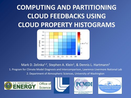
COMPUTING AND PARTITIONING<br />
CLOUD FEEDBACKS USING<br />
CLOUD PROPERTY HISTOGRAMS<br />
Mark D. Zelinka 1,2 , Stephen A. Klein 1 , & Dennis L. Hartmann 2<br />
1. Program <strong>for</strong> Climate Model Diagnosis <strong>and</strong> Intercomparison, Lawrence Livermore National Lab<br />
2. Department of Atmospheric Sciences, University of Washington
Goals<br />
• To provide a clean <strong>and</strong> simple method of computing cloud<br />
feedbacks that is highly in<strong>for</strong>mative<br />
• Clean:<br />
– compute cloud feedback from ISCCP simulator-interpreted cloud<br />
changes directly (not inferred)<br />
– st<strong>and</strong>ard definition of “cloud” <strong>and</strong> radiation code across models<br />
• Simple:<br />
– no need to correct <strong>for</strong> non-cloud effects<br />
– no partial radiative perturbation calculations are needed<br />
– can use monthly mean model output<br />
• In<strong>for</strong>mative:<br />
– can quantify the contribution to cloud feedback from changing<br />
amounts of individual cloud types (high, middle, low) <strong>and</strong> from<br />
individual processes (Δaltitude, Δoptical depth, Δtotal amount)
Data & Methodology<br />
• Doubled CO 2 equilibrium slab ocean model simulations from 12 GCMs<br />
as part of CFMIP1<br />
• ISCCP simulator run inline during integration<br />
– Produce distribution of cloud fraction (as function of CTP <strong>and</strong> τ) that is<br />
consistent with how a satellite-borne passive sensor would “view” the<br />
model atmosphere<br />
– Simulated cloud fractions are defined consistently across models<br />
• We compute cloud radiative kernels sensitivity of TOA radiation to<br />
cloud fraction changes in each CTP-τ bin<br />
• <strong>Cloud</strong> feedback = Δcloud fraction times cloud kernel normalized by ΔT sfc
Recipe <strong>for</strong> Constructing<br />
<strong>Cloud</strong> Radiative Kernels<br />
Input model mean zonal mean T <strong>and</strong> q profiles to Fu-Liou code<br />
Compute clear-sky TOA fluxes<br />
Compute overcast-sky fluxes <strong>for</strong> each CTP <strong>and</strong> τ bin by setting the<br />
LWC / IWC profiles to values appropriate <strong>for</strong> each cloud type<br />
Subtract overcast TOA fluxes in each bin from the clear-sky flux<br />
to compute a histogram of overcast sky cloud <strong>for</strong>cing<br />
Divide by 100 to get W m -2 % -1<br />
Repeat every calculation <strong>for</strong> 24 solar zenith angles, all latitudes,<br />
12 months, <strong>and</strong> 10 surface albedo bins between 0 <strong>and</strong> 1
Global Annual Mean <strong>Cloud</strong> Kernels<br />
CTP (hPa) CTP (hPa) CTP (hPa)<br />
LW<br />
SW<br />
Net<br />
τ<br />
W m -2 % -1<br />
W m -2 % -1<br />
W m -2 % -1
1xCO 2<br />
2xCO 2<br />
Change<br />
-0.4 % K -1<br />
CTP (hPa) CTP (hPa) CTP (hPa)<br />
<strong>Cloud</strong> Fraction<br />
τ<br />
x <strong>Cloud</strong> Radiative Kernels<br />
at each location <strong>and</strong> month,<br />
then averaged annually,<br />
globally, <strong>and</strong> across models…
1xCO 2<br />
2xCO 2<br />
Change<br />
-0.4 % K -1<br />
CTP (hPa) CTP (hPa) CTP (hPa)<br />
<strong>Cloud</strong> Fraction<br />
τ τ<br />
<strong>Cloud</strong> Feedback<br />
LW<br />
0.27 Wm -2 K -1<br />
SW<br />
0.44 Wm -2 K -1<br />
Net<br />
0.71 Wm -2 K -1
LW<br />
SW<br />
Net<br />
<strong>Cloud</strong> Kernel Adjusted ΔCRF<br />
Kernel minus<br />
Adjusted ΔCRF<br />
0.27 W m -2 K -1 0.21 W m -2 K -1 0.06 W m -2 K -1<br />
0.44 W m -2 K -1 0.44 W m -2 K -1 -0.01 W m -2 K -1<br />
0.70 W m -2 K -1 0.65 W m -2 K -1 0.04 W m -2 K -1
LW <strong>Cloud</strong> Kernel<br />
(W m-2 K-1 )<br />
SW <strong>Cloud</strong> Kernel<br />
(W m-2 K-1 )<br />
HadSM4 HadSM3 HadGSM1<br />
1.05<br />
1.02<br />
R 2 : 87%<br />
UIUC LOSENS CCCMA<br />
0.84<br />
0.83<br />
R 2 : 74%<br />
HadSM4 1.12 HadSM3 HadGSM1<br />
1.11<br />
R 2 : 95%<br />
R 2 : 89%<br />
R 2 : 48%<br />
R 2 : 97%<br />
UIUC 1.53 LOSENS 1.00 CCCMA 1.06<br />
Adjusted ΔCRF (W m -2 K -1 )<br />
0.97<br />
R 2 : 80%<br />
1.22<br />
R 2 : 87%<br />
1.14<br />
R 2 : 94%<br />
R 2 : 88% R 2 : 61% R 2 : 94%
• LW • Net • SW
Mean<br />
Cfrac<br />
Σ=52.5 %<br />
ΔAmount<br />
Σ=-0.42 %K -<br />
1<br />
Δτ<br />
Σ=0 % K -1<br />
τ τ<br />
• Decompose the cloud changes into<br />
ΔAMOUNT<br />
ΔALTITUDE<br />
ΔOPTICAL DEPTH<br />
ΔCfrac<br />
Σ=-0.42 %K -<br />
1<br />
ΔAltitude<br />
Σ=0 % K -1<br />
Residual<br />
Σ=0 % K -1
Mean<br />
Cfrac<br />
Σ=52.5 %<br />
ΔAmount<br />
Σ=-0.42 %K -<br />
1<br />
Δτ<br />
Σ=0 % K -1<br />
τ τ<br />
ΔCfrac<br />
Σ=-0.42 %K -<br />
1<br />
ΔAMOUNT = cloud fraction altered<br />
in proportion to amount in 1xCO2 histogram; no change in vertical or<br />
optical depth distribution<br />
ΔAltitude<br />
Σ=0 % K -1<br />
Residual<br />
Σ=0 % K -1
Mean<br />
Cfrac<br />
Σ=52.5 %<br />
ΔAmount<br />
Σ=-0.42 %K -<br />
1<br />
Δτ<br />
Σ=0 % K -1<br />
τ τ<br />
ΔALTITUDE = anomalous vertical<br />
distribution within each τ bin<br />
ΔCfrac<br />
Σ=-0.42 %K -<br />
1<br />
ΔAltitude<br />
Σ=0 % K -1<br />
Residual<br />
Σ=0 % K -1<br />
ΔOPTICAL DEPTH = anomalous optical<br />
depth distribution within each CTP bin
Mean<br />
Cfrac<br />
Σ=52.5 %<br />
ΔAmount<br />
Σ=-0.42 %K -<br />
1<br />
Δτ<br />
Σ=0 % K -1<br />
τ τ<br />
ΔCfrac<br />
Σ=-0.42 %K -<br />
1<br />
ΔAltitude<br />
Σ=0 % K -1<br />
Residual<br />
Σ=0 % K -1
Amount<br />
-0.30 W m -2 K -1<br />
Optical Depth<br />
0.16 W m -2 K -1<br />
LW <strong>Cloud</strong> Feedback<br />
0.26 W m -2 K -1<br />
Altitude<br />
0.44 W m -2 K -1<br />
Residual<br />
-0.04 W m -2 K -1
Amount<br />
0.66 W m -2 K -1<br />
Optical Depth<br />
-0.05 W m -2 K -1<br />
SW <strong>Cloud</strong> Feedback<br />
0.46 W m -2 K -1<br />
Altitude<br />
-0.03 W m -2 K -1<br />
Residual<br />
-0.11 W m -2 K -1
Amount<br />
0.36 W m -2 K -1<br />
Optical Depth<br />
0.09 W m -2 K -1<br />
Net <strong>Cloud</strong> Feedback<br />
0.71 W m -2 K -1<br />
Altitude<br />
0.41 W m -2 K -1<br />
Residual<br />
-0.15 W m -2 K -1
• LW • Net • SW
Conclusions (1 of 2)<br />
• <strong>Cloud</strong> radiative kernels allow computation of cloud feedback directly<br />
from cloud property histograms generated by ISCCP simulator<br />
– St<strong>and</strong>ard radiative transfer <strong>and</strong> definition of “cloud” across models<br />
– Non-cloud changes are automatically excluded (no adjustments necessary)<br />
– Relatively simple calculation (multiply two matrices) on monthly mean output<br />
– Ability to quantify contribution to feedback from individual cloud types<br />
• Feedbacks computed with cloud kernels compare very well with those<br />
computed by adjusting the change in cloud <strong>for</strong>cing [Soden et al. (2008)]<br />
• Ensemble (10 model) mean results:<br />
– LW <strong>and</strong> SW cloud feedbacks are positive, with SW nearly twice as as large as LW<br />
– More than half of the global mean net cloud feedback can be attributed to the<br />
combined response of middle- <strong>and</strong> high-level clouds<br />
– High cloud changes induce wider range of LW <strong>and</strong> SW cloud feedbacks across<br />
models than do low clouds
Conclusions (2 of 2)<br />
• Increasing cloud top altitude is dominant contributor to the positive<br />
global mean LW <strong>and</strong> net cloud feedbacks (positive in every model)<br />
– Positive impact of rising clouds is 50% larger than negative impact of reductions in<br />
cloud amount on LW cloud feedback (but varies considerably across models)<br />
• Decreasing total cloud fraction is dominant contributor to global mean<br />
positive SW cloud feedback (positive in every model)<br />
– Inter-model spread is greater than <strong>for</strong> any other feedback component<br />
– Overall cloud amount reductions have 2x as large an impact on SW as on LW fluxes<br />
• Large negative net cloud feedback at high latitudes is caused by<br />
increased optical depth, not increased cloud amount<br />
– Results from increased cloud water content <strong>and</strong> phase changes from ice to liquid<br />
• Draft of paper: email zelinka1@llnl.gov or Google “Mark Zelinka”


