Harmonious Hashing

Harmonious Hashing
Bin Xu 1 , Jiajun Bu 1 , Yue Lin 2 Chun Chen 1 , Xiaofei He 2 , Deng Cai 2
1 Zhejiang Provincial Key Laboratory of Service Robot,
College of Computer Science, Zhejiang University, China
{xbzju,bjj,chenc}@zju.edu.cn
2 State Key Lab of CAD&CG, College of Computer Science, Zhejiang University, China
linyue29@gmail.com, {xiaofeihe,dengcai}@cad.zju.edu.cn
Abstract
Hashing-based fast nearest neighbor search technique
has attracted great attention in both research
and industry areas recently. Many existing hashing
approaches encode data with projection-based hash
functions and represent each projected dimension
by 1-bit. However, the dimensions with high variance
hold large energy or information of data but
treated equivalently as dimensions with low variance,
which leads to a serious information loss. In
this paper, we introduce a novel hashing algorithm
called Harmonious Hashing which aims at learning
hash functions with low information loss. Specifically,
we learn a set of optimized projections to
preserve the maximum cumulative energy and meet
the constraint of equivalent variance on each dimension
as much as possible. In this way, we could
minimize the information loss after binarization.
Despite the extreme simplicity, our method outperforms
superiorly to many state-of-the-art hashing
methods in large-scale and high-dimensional nearest
neighbor search experiments.
1 Introduction
In managing or mining massive databases with millions of
data samples and thousands of features, fast approximate
nearest neighbor (ANN) search is one of the most fundamental
and important techniques in many machine learning
and data mining problems, such as retrieval, classification
and clustering [Muja and Lowe, 2009; Jégou et al., 2011;
Hajebi et al., 2011]. Among various fast ANN search solutions,
hashing-based technique has attracted great attention
in past years. It has been actively studied, for both research
and industry purposes, due to its substantially reduced storage
cost and sub-linear query time.
Many existing hashing approaches encode data via
projection-based hash functions and generate binary codes
by thresholding. They try to preserve the pairwise distance
(e.g., Euclidean distance) of data samples on the original
space by Hamming distance on the obtained binary feature
space. Locality-Sensitive Hashing (LSH) [Indyk and
Motwani, 1998; Charikar, 2002], and its kernelized version
Normalized variance
16
14
12
10
8
6
4
2
1
0
1 10 20 30 40 50 60 70 80 90 100 110 120128
Dimension of projected data
SH
Ours
Precision of the first 100 samples
0.7
0.65
0.6
0.55
0.5
0.45
0.4
0.35
0.3
0.25
0.2
0.15
0.1
0.05
0
16 32 48 64 96 128
# of bits
SH
Ours
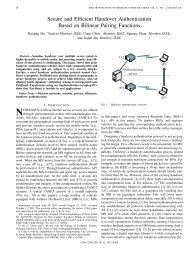
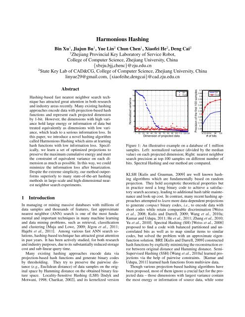
Figure 1: An illustrative example on a database of 1 million
samples. Left: normalized variance (divided by the median
value) on each projected dimension; Right: nearest neighbor
search precision at top-100 samples on different number of
bits. Spectral Hashing and our method are compared.
KLSH [Kulis and Grauman, 2009] are well known hashing
algorithms which are fundamentally based on random
projection. They hold asymptotic theoretical properties but
in practice need a long binary code to achieve a satisfactory
search accuracy, leading to additional hash table maintenance
and look-up cost. In contrast, many recent hashing approaches
attempted to learn more data-dependent projections
to generate compact binary codes, i.e., to encode data with
short codes while retain comparable discrimination [Weiss
et al., 2008; Kulis and Darrell, 2009; Wang et al., 2010a;
Kumar and Udupa, 2011; He et al., 2011; Zhang et al., 2010;
Yu et al., 2010]. Spectral Hashing (SH) [Weiss et al., 2008]
proposed to find a code with balanced partitioned and uncorrelated
bits as well as to map similar items to similar
codes, but solved the problem with an approximate eigenfunction
solution. BRE [Kulis and Darrell, 2009] constructed
hash functions by explicitly minimizing the reconstruction error
between original distance and Hamming distance. Semi-
Supervised Hashing (SSH) [Wang et al., 2010a] learned projections
via the help of pairwise constraints. [Kumar and
Udupa, 2011] learned hash functions from multiview data.
Though various projection-based hashing algorithms have
been proposed, most of them ignore a crucial fact for the projected
data – those dimensions with largest variance contain
the most energy or information of source data, while some

other dimensions are less informative. However, each dimension
is encoded into 1-binary bit and the Hamming distance
has equivalent weight on each bit, no matter what the original
dimension is, i.e., there is a serious information loss for the
dimensions with high variance. A few recent researches have
considered this unbalanced problem. In [Wang et al., 2010b],
the authors firstly claimed that this problem decreased the
search performance substantially. To address it, they learned
the bit-correlated hash functions sequentially and each new
bit was to correct the errors made by previous bits. However
such a greedy algorithm would be dependent on the selection
of true (or pseudo) labels and how to get the labels is also a
problem. Liu et al. designed a two-layer hashing function to
represent each top dimension (eigenvector) by 2 bits to avoid
the influence of low quality dimensions [Liu et al., 2011].
However the performance of the heuristic setting of 2-bit depends
on the data distribution and using 2-bit means that we
could only use half of the projections, losing the information
in the rest.
Different with the previous works, in this paper we propose
a novel hashing method called Harmonious Hashing
(HamH), which aims at learning hash functions with minimum
information loss. The main idea is to adjust the projected
data for uniform energy distribution on each dimension.
Specifically, we learn a set of optimized projections
which hold the maximum cumulative energy and meet the
constraint of equivalent variance on each dimension as much
as possible. In this way, we could preserve the maximum
energy and minimize the information loss after binarization.
Our method has a non-iterative and closed form solution.
More detailedly, our Harmonious Hashing algorithm is
derived from the original eigenvector definition of Spectral
Hashing but outperforms it a lot in our large-scale and highdimensional
nearest neighbor search experiments. Fig.1 is
an illustrative example on GIST1M database with 1 million
data samples. We plot the normalized variance (divided by
the median value) on each (continuous) projected dimension.
For Spectral Hashing (blue dot, sorted), the variance varies in
a large range, while for our method, it is more uniform – the
normalized variance is distributed around 1. As a result, the
performance of our method is much better. Besides Spectral
Hashing, our method is comparable or outperforms to many
state-of-the-art hashing methods in our experiments.
2 Preliminaries
Our work comes of the eigenvector formulation of Spectral
Hashing. In this section, we briefly review and analyze it.
2.1 Spectral Hashing
Given a data set X = [x1, x2, . . . , xn] T ∈ R n×m with n
samples and each row x T i ∈ Rm is a m-dimensional data
vector. Let Y = [y1, y2, . . . , yn] T ∈ R n×k be the k-bit
Hamming embedding (binary codes of length k) for all the
samples and An×n be the symmetric weight matrix. To seek
a qualified code, Spectral Hashing requires each bit to have
half number of +1 or −1 and the bits to be uncorrelated to
each other, as well as maps similar samples to similar binary
codes. Its objective function can be written as:
min
tr(Y T LY )
Y
s.t. Y (i, j) ∈ {−1, 1}
Y T 1 = 0
Y T Y = I
where L = D − A is the graph Laplacian [Chung, 1997] and
D is a diagonal matrix with Dii =
j Aij and 1 (0) is a
column vector with all ones (zeros).
It was stated that even for a single bit (k = 1), solving
problem (1) is equivalent to balanced graph partitioning
and is NP hard [Weiss et al., 2008]. For k-bits the problem
is even harder, but by removing the binary constraint
Y (i, j) ∈ {−1, 1} to make Y continuous, the optimization
becomes a well-studied problem whose solutions are the k
eigenvectors of L with minimal eigenvalues. Then simply
thresholding these eigenvectors to generate balanced binary
codes. Though this approach is very intuitive, it can only
compute the codes of items in the database (training data) but
not for an out-of-sample, i.e., a new query sample. Instead of
solving the eigenvector solution, Spectral Hashing adopted
an approximate eigenfunction solution with the assumption
of uniform data distribution. The eigenfunction solution is
not the focus of our work, thus we skip it here.
Beside those very recent related work in Section 1, we also
find some interesting clues in Spectral Hashing (SH) [Weiss
et al., 2008]. The authors said ’using PCA to align the axes,
and assuming an uniform distribution on each axis works surprisingly
well...’. Although this discovery is very interesting
and useful, the authors failed to offer further analysis to it
but just make an eigenfunction extension for learning out-ofsample
codes. Many later methods were inspired by Spectral
Hashing’s original eigenvector formulation or the eigenfunction
extension, but none of them have analyzed this issue theoretically.
In the analysis of our model (Section 3.4), We find
that the idea of uniform (energy) distribution is hidden in the
original definition of Spectral Hashing.
3 Harmonious Hashing
3.1 A Naive Extension of Spectral Hashing
We propose a naive out-of-sample extension of Spectral
Hashing from its relaxed eigenvector formulation. This naive
approach is the origin of our Harmonious Hashing algorithm.
Without loss of generality, for the rest of this paper,
we assume that the data samples are zero-centered, i.e.,
n
i=1 xi = 0, and the affinity matrix is calculated by its symmetric
normalization, then we have:
à = D −1/2 AD −1/2
(1)
(2)
˜L = I − Ã (3)
where ˜ L is the normalized graph Laplacian. For out-ofsample
extension, let the k-dimensional embedding Y be calculated
by k linear projections from original data X, i.e.,
Y = XW , W ∈ R m×k and each column of W is a projection
vector. Substituting the linear projection and the normalized

graph Laplacian into the relaxed continuous version of problem
(1) and replacing the orthogonal constraint, we could get
a naive out-of-sample extension of Spectral Hashing as:
max
W
tr(W T X T ÃXW )
s.t. W T X T 1 = 0
W T W = I.
The constraint W T X1 = 0 always holds since the data is
zero-centered. Thus the solutions of problem (4) are the k
eigenvectors of the matrix XT ÃX with maximal eigenvalues.
By this way, we could compute the binary code for both
training data and query data in the same manner: projecting
the data by Y = XW and thresholding at zero for each bit.
As this method is a naive extension of Spectral Hashing, we
denote it by nSH for short.
However, there remains a critical problem for both SH and
nSH – traditional constructing method for the affinity matrix
A is costly for a large database, e.g., building a kNN graph
has a complexity of O(n2 log k). Though it is computed offline,
for millions of samples, the computation is too slow.
Thus for the nSH algorithm, we adopt to build a landmarkbased
graph, or an anchor graph which has been proved to
be efficient and effective in many recent work [Zhang et al.,
2009; Liu et al., 2010; Xu et al., 2011; Lin et al., 2012; Lu
et al., 2012]. Let U = {u1, . . . , ud} ⊂ Rm denote a set of
d landmarks sampled from the database. To build the anchor
graph based on the landmarks, we essentially find the sparse
weight matrix Z ∈ Rn×d so that each data sample can be
approximated by its nearby landmarks:
xi ≈
ujzij, (5)
j∈N 〈i〉
where N 〈i〉 denotes the index set of s nearest landmarks of
xi. We compute zij by kernel regression method:
K(xi, uj)
zij =
j ′ ∈N K(xi, uj
〈i〉 ′),
where K is a pre-given kernel function [Xu et al., 2011; Lin et
al., 2012]. Solving Z has a complexity of O(nd log s). Then
the affinity matrix is calculated by a low-rank formulation as
A = ZZ T and its normalization is
(4)
(6)
à = D −1/2 ZZ T D −1/2 = HH T , (7)
where H = D −1/2 Z. As a result, we could re-write the
objective function of nSH as:
max
W
s.t. W T W = I.
tr(W T X T HH T XW )
Through in-depth analysis of problem (8), we receive the
main idea of our method. We describe it in the next section.
3.2 Observation and Motivation
We first introduce the definition of cumulative energy:
Definition Let C ∈ R m×m be the covariance matrix of
any data set, its full eigen-decomposition can be written as
(8)
C = UΛU T where Λ is the diagonal matrix of sorted eigenvalues
of C, i.e., Λii = λi and λ1 ≥ λ2 ≥, . . . , ≥ λm. The
eigenvalues represent the distribution of the source data’s energy
among each of the eigenvectors. Then the cumulative
energy content g for the k-th eigenvector is the sum of the
energy content across all of the first k eigenvalues:
gk(C) =
k
|Λii| (9)
i=1
Now going back to problem (8), let ˜ C = X T HH T X,
which plays a very similar role as the covariance matrix but
integrates more graph-based structure information. We name
it as graph covariance matrix. The solution of problem (8)
for k-bit embedding is the top-k eigenvectors of ˜ C with maximal
eigenvalues, forming the matrix W ∗ ∈ R m×k . ˜ C is a
positive semi-definite matrix, i.e., all of its eigenvalues are
nonnegative, then the object of problem (8) is formulated as
tr(W ∗T ˜ CW ∗ ) = tr( ˜ Λ) =
k
˜Λii = gk( ˜ C), (10)
i=1
which indicates that to solve the problem of (8), we essentially
find a set of k eigenvectors holding the maximum cumulative
energy. An intuitive next step would be projecting
the source data by W ∗ , i.e., Y = XW ∗ , and then thresholding
at zero (or median) to obtain the binary codes, just as
most traditional hashing methods did.
However this approach ignores a crucial fact of the projected
data Y – the top dimensions hold the most energy of
source data while the rest dimensions keep much less energy,
since the eigenvalue decreases dramatically for many
real data. From another point, we could observe the variance
of the projected data: the top dimensions have large variances
while the rest are much smaller. The variance of one dimension
reflects its energy or information of the data. However,
each dimension is represented by 1-binary bit equivalently.
As a result, some bits are energy overloaded and some are
less informative. Hamming distance has equivalent weight
on each bit, i.e., general projected data does not match the
Hamming distance metric well.
To solve the problem above, we propose a novel approach
which preserves the maximum cumulative energy, and at
the same time allocates the energy into each projection uniformly
by restricting the variance of each projected dimension
equally. We adopt a non-iterative algorithm to solve it.
3.3 Learning Algorithm
It is observed that, if W is an optimal solution of problem (8),
then so is ˜ W = W E with E ∈ R k×k an arbitrary orthogonal
matrix (E T E = EE T = I), since
tr(E T W T ˜ CW E) = tr(W T ˜ CW ) = gk( ˜ C). (11)
That is to say, there is an infinite set of (continuous) projected
data in the form of Y = XW E, that can preserve the maximum
cumulative energy. Our objective is to find some Y in
this set with equivalent variance on each dimension to guarantee
uniform energy distribution. We design a loss function

as:
Q(Y, E) = Y − XW E 2 F
s.t. Y T Y = Diag(σ1)
E T E = I,
(12)
where Diag(σ1) is a diagonal matrix with each diagonal element
equal to the scalar σ and · F is the Frobenius norm
of a matrix. σ is a specific variance value but we just denote
it by a symbol now and discuss its effect later in Section 3.4.
By observation, we find that given any arbitrary orthogonal
matrix E0 , we could get an optimal Y fitting the object by
solving the following single problem:
min Y − XW E0
Y
2 F
s.t. Y T Y = Diag(σ1).
(13)
That is to say, there is still an infinite candidate set of Y holding
the maximum cumulative energy and equivalent variance.
But in other words, any Y in this set is qualified for our object,
thus we just pick one of them. Solving the single problem
(13), we should use the following theorem.
Theorem 3.1 Given any real valued matrix Y ∈ R n×k and
V ∈ R n×k (n ≥ k), and any real valued vector u ∈ R k ≥ 0,
suppose the singular value decomposition of V is V = P ∆Q,
then the optimal solution to the following problem is Y ∗ =
P Diag( √ u)Q, where Diag(·) is a diagonal matrix.
min Y − V
Y
2 F
s.t. Y T Y = Diag(u).
(14)
The proof of this theorem is presented in the Appendix.
Let V = XW E0 (any arbitrary orthogonal matrix E0), the
optimal solution of problem (13) is Y ∗ = √ σP Q.
With the fixed Y ∗ , we want to find an unique optimal E by
minimizing the reconstruction error of problem (12), i.e., to
solve a second single problem as:
min
E
s.t. ET E = I,
Y ∗ − XW E 2 F
(15)
whose optimal solution is E ∗ = GS, where G and S are the
left and right singular vectors of the k × k matrix W T X T Y ∗ ,
i.e., W T X T Y ∗ = GΣS, which has been investigated in
some previous works [Yu and Shi, 2003; Chen et al., 2011;
Gong and Lazebnik, 2011]
NOTE: since picking any Y in the infinite set meeting
our object has almost the same effect to uniformly distribute
the data energy along each dimension, our optimization algorithm
for problem (12) is non-iterative. It stops when we
solve E ∗ of problem (15) for the first time, which guarantees
the light weight of the optimization.
By now, we have obtained a k-bit data embedding as
Y = XW E ∗ for the in-sample data X (training data), where
W is the top-k eigenvectors of ˜ C and E ∗ is the solution of
problem (15), then we cut Y at zero to get the binary codes.
For any out-of-sample query data xq, we use the same strategy
to generate its binary code bq, i.e.,
bq = (sgn(xqW E ∗ ) + 1)/2. (16)
3.4 Analysis
Let’s consider the value of variance σ for each dimension of
Y , which represents a corresponding degree of energy. A
natural conclusion is that: when the maximum energy of all
the dimensions is fixed, asking each dimension’s energy to
be equal to each other has the same effect to constrain each
energy to be a specific value. This can be observed from our
optimization algorithm above. As Y ∗ = √ σP Q, the value of
σ only does a scaling to Y ∗ , as well as to the value of Σ but
not to G and S in the SVD of W T X T Y ∗ = GΣS. As a result,
E ∗ remains the same no matter what the σ is. We could
just set σ to 1 for simplicity, i.e., Y T Y = I. Surprisingly, we
find this constraint appeared in the relaxed eigenvector definition
of Spectral Hashing – the authors said it is to enforce the
bits to be uncorrelated, but a hidden effect is to make the variance
on each dimension equally, as well as the energy, which
conforms with the idea of our Harmonious Hashing model.
However the eigenfunction solution of Spectral Hashing lost
this constraint.
Two very recent hashing algorithms Iterative Quantization
(ITQ) [Gong and Lazebnik, 2011] and Isotropic Hashing
(IsoH) [Kong and Li, 2012] have close relationship to our
model. ITQ balances the variance on each dimension by iteratively
minimizing the quantization error, but its local optimum
cannot guarantee equivalent variance. IsoH iteratively
minimizes the reconstruction error of the the covariance matrix
and a diagonal matrix, but their optimization on the small
covariance matrix seems to be too restricted – the algorithm
is unstable in large-scale and high-dimensional experiments.
Moreover, both ITQ and IsoH focus on PCA-projections,
while we derive our algorithm from Spectral Hashing, which
utilizes more data structure information.
4 Experimental Results
In this section, we evaluate the performance of our method for
nearest neighbor search task on two real world large-scale and
high-dimensional databases GIST1M and ImageNet, and
compare with many state-of-the-art hashing approaches. Our
experiments are implemented on a computer with double 2.0
GHz CPU and 64GB RAM.
4.1 Date Statistics and Experimental Setup
• GIST1M database has 1 million GIST descriptors from
the web 1 . It is a well known database for the task of approximate
nearest neighbor search. Each GIST descriptor
(one sample) is a dense vector of 960 dimensions.
• ImageNet is an image database organized according to
the WordNet nouns hierarchy, in which each node of the
hierarchy is depicted by hundreds and thousands of images
2 . We downloaded about 1.2 million images’ BoW
representations from 1,000 nodes. A visual vocabulary
of 1,000 visual words is adopted, i.e., each image is represented
by a 1,000-length sparse vector.
For both of the two databases, we randomly select 1,000 data
samples as out-of-sample test queries and the rest samples
1 http://corpus-texmex.irisa.fr/
2 http://www.image-net.org/index

Precision
0.5
0.45
0.4
0.35
0.3
0.25
0.2
0.15
0.1
HamH
ITQ
IsoH
KLSH
AGH
LSH
SH
0.05
100 500 1000 2000 3000
# of retrieved samples
5000
(a) 32 bits
Precision
0.6
0.55
0.5
0.45
0.4
0.35
0.3
0.25
0.2
0.15
HamH
ITQ
IsoH
KLSH
AGH
LSH
SH
0.1
100 500 1000 2000 3000
# of retrieved samples
5000
(b) 64 bits
Precision
0.6
0.55
0.5
0.45
0.4
0.35
0.3
0.25
0.2
0.15
HamH
ITQ
IsoH
KLSH
AGH
LSH
SH
0.1
100 500 1000 2000 3000
# of retrieved samples
5000
(c) 96 bits
Precision
0.6
0.55
0.5
0.45
0.4
0.35
0.3
0.25
0.2
0.15
HamH
ITQ
IsoH
KLSH
AGH
LSH
SH
0.1
100 500 1000 2000 3000
# of retrieved samples
5000
(d) 128 bits
Figure 2: Precision at different number of retrieved samples on GIST1M database with 32, 64, 96 and 128 bits respectively.
Precision
0.4
0.35
0.3
0.25
0.2
0.15
HamH
ITQ
IsoH
KLSH
AGH
LSH
SH
0.1
100 500 1000 2000 3000
# of retrieved samples
5000
(a) 32 bits
Precision
0.5
0.45
0.4
0.35
0.3
0.25
0.2
0.15
HamH
ITQ
IsoH
KLSH
AGH
LSH
SH
0.1
100 500 1000 2000 3000
# of retrieved samples
5000
(b) 64 bits
Precision
0.6
0.55
0.5
0.45
0.4
0.35
0.3
0.25
0.2
HamH
ITQ
IsoH
KLSH
AGH
LSH
SH
0.15
100 500 1000 2000 3000
# of retrieved samples
5000
(c) 96 bits
Precision
0.6
0.55
0.5
0.45
0.4
0.35
0.3
0.25
0.2
HamH
ITQ
IsoH
KLSH
AGH
LSH
SH
0.15
100 500 1000 2000 3000
# of retrieved samples
5000
(d) 128 bits
Figure 3: Precision at different number of retrieved samples on ImageNet database with 32, 64, 96 and 128 bits respectively.
Table 1: Basic statistics of the two databases.
GIST1M ImageNet
# of samples 1,000,000 1,261,406
# of dimensions 960 1,000
is sparse no yes
are treated as training data. Some basic statistics of the two
databases are listed in Table 1.
To evaluate the performance of nearest neighbor search, we
should first obtain the groundtruth neighbors. Following the
criterion used in many previous works [Weiss et al., 2008;
Wang et al., 2010a; 2010b], the groundtruth neighbors are
obtained by brute force search with Euclidean distance. A
data sample is considered to be a true neighbor if it lies in the
top-1 percent samples closest to the query.
To run our model, we build a landmark-based graph. We
should determine the number of landmarks, the local size s
of nearby landmarks and the kernel function. However from
experiments, we find that the model HamH is not sensitive to
the parameters (since all the graph information is embedded
in a small graph covariance matrix ˜ C). In all of our experiments
below, we fix all the parameters the same as [Xu et
al., 2011], i.e., we use the quadratic kernel and set s = 5.
We select landmarks randomly form the training data and the
number is fixed to be twice the number of binary bits, i.e., for
a 32-bit code, we use 64 landmarks. The random selection
procedure and fixed number of landmarks can guarantee the
efficiency as well as the robustness of our model.
4.2 Compared Approaches
We compare the proposed Harmonious Hashing (HamH) algorithm
with the following state-of-the-art hashing methods:
• SH: Spectral Hashing [Weiss et al., 2008].
• LSH ⋆ : Locality-Sensitive Hashing [Charikar, 2002].
We generated the random projections via a (0, 1) normal
distribution.
• KLSH: Kernelized Locality-Sensitive Hashing [Kulis
and Grauman, 2009], constructing random projections
using the kernel function and a set of examples.
• AGH: Anchor Graph Hashing [Liu et al., 2011] with
two-layer hash functions generates r bits actually use the
r/2 lower eigenvectors twice.
• ITQ: Iterative Quantization [Gong and Lazebnik, 2011],
minimizing the quantization loss by rotating the PCAprojected
data.
• IsoH ⋆ : Isotropic Hashing [Kong and Li, 2012], learning
projection functions with isotropic variances for PCAprojected
data. We implemented the Lift and Projection
algorithm to solve the optimization problem.
Among these approaches, LSH and KLSH are random projection
methods and the others are learning-based methods.
ITQ and IsoH are two very recent proposed hashing methods
with close relationship to our method. The methods with ⋆
are implemented by ourselves strictly according to their papers
and the others are provided by the original authors.
4.3 Results
We first compute the precision (percent of true neighbors)
under the Hamming ranking evaluation, i.e., the Hamming
distance of the query and each database sample is calculated
and sorted. The precision values at different number of retrieved
samples are recorded in Fig.2 and Fig.3. We vary the
length of binary codes from 32 bits to 128 bits to see the
performance of all the methods on compact codes and relatively
long codes. Despite the simplicity of our method, it

Precision of the first 500 samples
0.5
0.45
0.4
0.35
0.3
0.25
0.2
HamH
ITQ
0.15
IsoH
KLSH
0.1
AGH
0.05
LSH
SH
0
16 32 48 64
# of bits
96 128
(a) GIST1M database
Precision of the first 500 samples
0.5
0.45
0.4
0.35
0.3
0.25
0.2
HamH
ITQ
0.15
IsoH
KLSH
0.1
AGH
0.05
LSH
SH
0
16 32 48 64
# of bits
96 128
(b) ImageNet database
Figure 4: Precision at first 500 samples on different number
of bits on (a) GIST1M and (b) ImageNet databases.
Table 2: Training time (in seconds) of all the methods.
GIST1M ImageNet
32 bits 64 bits 128 bits 32 bits 64 bits 128 bits
HamH 201.05 208.72 228.83 313.62 331.10 371.02
ITQ 128.76 205.47 377.43 201.47 327.19 573.49
IsoH 34.17 35.27 40.77 59.05 60.53 65.60
KLSH 104.09 108.14 109.71 133.89 136.98 136.08
AGH 267.80 313.53 492.07 352.94 409.90 630.26
LSH 2.60 3.93 5.52 3.77 6.17 9.67
SpH 137.06 242.08 662.17 194.28 339.65 950.24
performs comparably to or outperforms the other methods on
each database and each code length, proving its effectiveness
and stability. As discussed in section 1, random projection
algorithms play well on a long code – KLSH achieves a high
precision on 96 or 128 bits but performs poorly on a short
code. Both GIST1M and ImageNet are large-scale and highdimensional,
but GIST1M has dense features and ImageNet
has sparse (BoW) features. Compare Fig.2 to Fig.3, some
methods performs better on the dense set while some others
performs better on the sparse set, i.e., they are sensitive to the
data characteristic. However, our method HamH focusing on
the data energy distribution is more robust – it performs well
on both sets. On the ImageNet database, IsoH performs almost
the second best on each code length. However, on the
GIST1M database, it seems to be unstable: IsoH performs
well on a short code but drops its precision on a long code.
In Fig.4, we plot the precision of the first 500 retrieved
samples on different length of binary bits. It can be seen that,
the algorithms perform differently on the dense and sparse
sets, while our method performs well on both sets.
Finally, we record the training time of all the methods in
Table 2. Our method HamH is at an intermediate level of
training cost. However, considering the large scale of the
databases and the training process running totally off-line, the
time of each method is acceptable. On the query process, they
have similar steps (projection and binarization), both very efficient,
so we skip the comparison.
5 Conclusion
We have designed an extremely simple but effective binary
code generating method Harmonious Hashing, which adjusts
the projected dimensions via uniform energy distribution.
With a non-iterative and efficient solution, our method out-
performs or is comparable to many state-of-the art methods
for nearest neighbor search experiments on large-scale and
high-dimensional databases. However, we find that with a
small code (32 or 64 bits), our method (as well as many other
learning-based algorithms) has arrived at a competitive level
of search accuracy, but improvement is limited when more
bits are adopted. From the view of data energy, the most energy
is kept in the top dimensions, so the later ones do not
help much. But for random projection methods, the situation
is totally opposite. How to combine learning projections and
random projections is an interesting future work.
6 Acknowledgments
This work was supported by National Basic Research Program
of China (973 Program) under Grant 2013CB336500,
National Natural Science Foundation of China: 61173186,
61222207, 61125203, 91120302, Scholarship Award for Excellent
Doctoral Student granted by Ministry of Education.
A Appendix
A.1 Proof of Theorem 3.1
To solve the problem (14), we introduce the Lagrange function
(with multipliers saved in Λ ∈ Rk×k ) defined as:
L(Y, Λ) = Y − V 2 F + tr(Λ(Y T Y − Diag(u))). (17)
Suppose Y ∗ is the optimal solution, according to the KKT
conditions, we have
Stationarity :
∂L
∂Yd
|Y =Y ∗ = 0, d = 1, . . . , k (17a)
P rimal F easibility : Y ∗T Y ∗ = Diag(u) (17b)
By Eq.(17a), we get V = Y ∗ Θ, where Θ = Λ + I is symmetric
since Y T Y − Diag(u) is symmetric. When k ≤ n,
assume Y ∗ and V are full column rank, then Θ is invertible.
Let the SVD of V be V = P ∆Q, then Y ∗ = P ∆QΘ −1 .
Substituting V and Y ∗ into the original object function, the
resulting objective is to maximize
O = tr(QΘ −1 Q T ∆ 2 ) = tr(H∆ 2 ) =
k
d=1
hddδ 2 dd, (18)
where H = QΘ −1 Q T . According to the Primal Feasibility:
Diag(u) = Y ∗T Y ∗ = QY ∗T Y ∗ Q T = H T ∆ 2 H. (19)
That is to say, for any d, k
j=1 h2 dj δ2 jj = ud and then
h 2 dd δ2 dd ≤ k
j=1 h2 dj δ2 jj = ud, thus
hddδdd ≤ √ ud. (20)
As a result, the object value of Eq.(18) has a upper bound of
k
O = hddδ 2 k √
dd ≤ udδdd. (21)
d=1
d=1
To achieve the maximum, for any d, the equality of Eq.(20)
holds, i.e., hdd = √ udδ −1
dd and hdj|j=d = 0, or
H = Diag( √ u)∆ −1 . (22)
Since H = QΘ−1QT , we could get the optimal solution as
Y ∗ = P ∆QΘ −1 = P ∆HQ = P Diag( √ u)Q. (23)
This theorem can be seen as a generalized version of theorem
2.1 in [Chen et al., 2011].

References
[Charikar, 2002] M.S. Charikar. Similarity estimation techniques
from rounding algorithms. In Proceedings of the
thiry-fourth annual ACM symposium on Theory of computing,
pages 380–388, 2002.
[Chen et al., 2011] X. Chen, Y. Qi, B. Bai, Q. Lin, and J.G.
Carbonell. Sparse latent semantic analysis. In SIAM 2011
International Conference on Data Mining, pages 474–485,
2011.
[Chung, 1997] F.R.K. Chung. Spectral graph theory, volume
92. Amer Mathematical Society, 1997.
[Gong and Lazebnik, 2011] Y. Gong and S. Lazebnik. Iterative
quantization: A procrustean approach to learning binary
codes. In IEEE Conference on Computer Vision and
Pattern Recognition, pages 817–824, 2011.
[Hajebi et al., 2011] K. Hajebi, Y. Abbasi-Yadkori, H. Shahbazi,
and H. Zhang. Fast approximate nearest-neighbor
search with k-nearest neighbor graph. In Proceedings of
the Twenty-Second international joint conference on Artificial
Intelligence, pages 1312–1317, 2011.
[He et al., 2011] J. He, R. Radhakrishnan, S.F. Chang, and
C. Bauer. Compact hashing with joint optimization of
search accuracy and time. In IEEE Conference on Computer
Vision and Pattern Recognition, pages 753–760,
2011.
[Indyk and Motwani, 1998] P. Indyk and R. Motwani. Approximate
nearest neighbors: towards removing the curse
of dimensionality. In Proceedings of the thirtieth annual
ACM symposium on Theory of computing, pages 604–613,
1998.
[Jégou et al., 2011] H. Jégou, M. Douze, and C. Schmid.
Product quantization for nearest neighbor search. IEEE
Transactions on Pattern Analysis and Machine Intelligence,
33(1):117–128, 2011.
[Kong and Li, 2012] W. Kong and W.J. Li. Isotropic hashing.
In Advances in Neural Information Processing Systems,
pages 1655–1663, 2012.
[Kulis and Darrell, 2009] B. Kulis and T. Darrell. Learning
to hash with binary reconstructive embeddings. Advances
in neural information processing systems, pages 1042–
1050, 2009.
[Kulis and Grauman, 2009] B. Kulis and K. Grauman. Kernelized
locality-sensitive hashing for scalable image
search. In IEEE International Conference on Computer
Vision, pages 2130–2137, 2009.
[Kumar and Udupa, 2011] S. Kumar and R. Udupa. Learning
hash functions for cross-view similarity search. In Proceedings
of the Twenty-Second international joint conference
on Artificial Intelligence, pages 1360–1365, 2011.
[Lin et al., 2012] Y. Lin, R. Jin, D. Cai, and X. He. Random
projection with filtering for nearly duplicate search.
In Proceedings of the Twenty-Sixth Conference on Artificial
Intelligence, pages 641–647, 2012.
[Liu et al., 2010] W. Liu, J. He, and S.F. Chang. Large graph
construction for scalable semi-supervised learning. In Proceedings
of the 27th International Conference on Machine
Learning, pages 679–686, 2010.
[Liu et al., 2011] W. Liu, J. Wang, S. Kumar, and S.F.
Chang. Hashing with graphs. In Proceedings of the 28th
International Conference on Machine Learning, pages 1–
8, 2011.
[Lu et al., 2012] Yao Lu, Wei Zhang, Ke Zhang, and Xiangyang
Xue. Semantic context learning with large-scale
weakly-labeled image set. In Proceedings of the 21st ACM
international conference on Information and knowledge
management, pages 1859–1863, 2012.
[Muja and Lowe, 2009] M. Muja and D.G. Lowe. Fast approximate
nearest neighbors with automatic algorithm
configuration. In International Conference on Computer
Vision Theory and Applications, pages 331–340, 2009.
[Wang et al., 2010a] J. Wang, S. Kumar, and S.F. Chang.
Semi-supervised hashing for scalable image retrieval. In
IEEE Conference on Computer Vision and Pattern Recognition,
pages 3424–3431, 2010.
[Wang et al., 2010b] J. Wang, S. Kumar, and S.F. Chang.
Sequential projection learning for hashing with compact
codes. In Proceedings of International Conference on Machine
Learning, pages 1127–1134, 2010.
[Weiss et al., 2008] Y. Weiss, A. Torralba, and R. Fergus.
Spectral hashing. Advances in neural information processing
systems, pages 1753–1760, 2008.
[Xu et al., 2011] B. Xu, J. Bu, C. Chen, D. Cai, X. He,
W. Liu, and J. Luo. Efficient manifold ranking for image
retrieval. In Proceedings of the 34th international ACM
SIGIR conference on Research and development in Information,
pages 525–534, 2011.
[Yu and Shi, 2003] S.X. Yu and J. Shi. Multiclass spectral
clustering. In IEEE International Conference on Computer
Vision, pages 313–319, 2003.
[Yu et al., 2010] Zhou Yu, Deng Cai, and Xiaofei He. Errorcorrecting
output hashing in fast similarity search. In Proceedings
of the Second International Conference on Internet
Multimedia Computing and Service, pages 7–10, 2010.
[Zhang et al., 2009] K. Zhang, J.T. Kwok, and B. Parvin.
Prototype vector machine for large scale semi-supervised
learning. In Proceedings of the 26th Annual International
Conference on Machine Learning, pages 1233–
1240, 2009.
[Zhang et al., 2010] Dell Zhang, Jun Wang, Deng Cai, and
Jinsong Lu. Self-taught hashing for fast similarity search.
In Proceedings of the 33rd international ACM SIGIR conference
on Research and development in information retrieval,
pages 18–25, 2010.