Madden–Julian Oscillation analog and intraseasonal variability in a ...

More documents

Recommendations

Info

$Lecture notes for Math 522 Spring 2012 (Rudin chapter 7)$

$Math 320 - Fall 2010 HW #7 Selected Solutions Problem 5.1.32 Let ...$

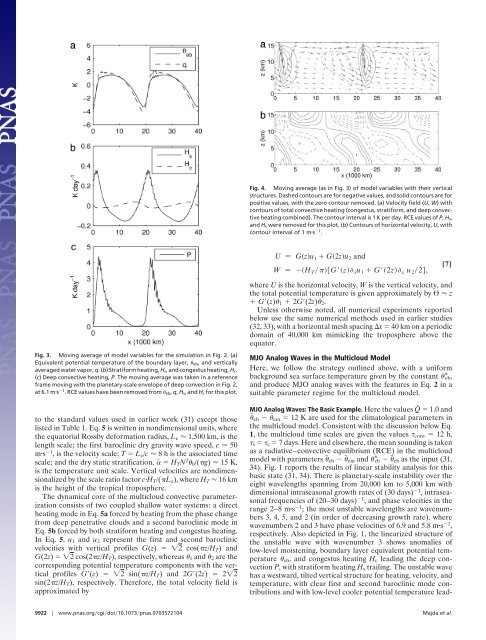
Fig. 3. Moving average of model variables for the simulation in Fig. 2. (a) Equivalent potential temperature of the boundary layer, eb, and vertically averaged water vapor, q.(b) Stratiform heating, Hs, and congestus heating, Hc. (c) Deep convective heating, P. The moving average was taken in a reference frame moving with the planetary-scale envelope of deep convection in Fig. 2, at 6.1 ms 1 . RCE values have been removed from eb, q, Hs, and Hc for this plot. to the standard values used in earlier work (31) except those listed in Table 1. Eq. 5 is written in nondimensional units, where the equatorial Rossby deformation radius, Le 1,500 km, is the length scale; the first baroclinic dry gravity wave speed, c 50 ms 1 , is the velocity scale; T Le/c 8 h is the associated time scale; and the dry static stratification, HTN 2 0/(g) 15 K, is the temperature unit scale. Vertical velocities are nondimensionalized by the scale ratio factor cHT/(Le), where HT 16 km is the height of the tropical troposphere. The dynamical core of the multicloud convective parameterization consists of two coupled shallow water systems: a direct heating mode in Eq. 5a forced by heating from the phase change from deep penetrative clouds and a second baroclinic mode in Eq. 5b forced by both stratiform heating and congestus heating. In Eq. 5, u1 and u2 represent the first and second baroclinic velocities with vertical profiles G(z) 2 cos(z/HT) and G(2z) 2 cos(2z/HT), respectively, whereas 1 and 2 are the corresponding potential temperature components with the vertical profiles G(z) 2 sin(z/HT) and 2G(2z) 22 sin(2z/HT), respectively. Therefore, the total velocity field is approximated by Fig. 4. Moving average (as in Fig. 3) of model variables with their vertical structures. Dashed contours are for negative values, and solid contours are for positive values, with the zero contour removed. (a) Velocity field (U, W) with contours of total convective heating (congestus, stratiform, and deep convective heating combined). The contour interval is 1 K per day. RCE values of P, Hs, and Hc were removed for this plot. (b) Contours of horizontal velocity, U, with contour interval of 1 ms 1 . U Gzu 1 G2zu 2 and W H TGz xu 1 G2z x u 22, [7] where U is the horizontal velocity, W is the vertical velocity, and the total potential temperature is given approximately by z G(z)1 2G(2z)2. Unless otherwise noted, all numerical experiments reported below use the same numerical methods used in earlier studies (32, 33), with a horizontal mesh spacing x 40 km on a periodic domain of 40,000 km mimicking the troposphere above the equator. MJO Analog Waves in the Multicloud Model Here, we follow the strategy outlined above, with a uniform background sea surface temperature given by the constant * eb, and produce MJO analog waves with the features in Eq. 2 in a suitable parameter regime for the multicloud model. MJO Analog Waves: The Basic Example. Here the values Q˜ 1.0 and eb em 12 K are used for the climatological parameters in the multicloud model. Consistent with the discussion below Eq. 1, the multicloud time scales are given the values conv 12 h, s c 7 days. Here and elsewhere, the mean sounding is taken as a radiative–convective equilibrium (RCE) in the multicloud model with parameters eb em and * eb eb as the input (31, 34). Fig. 1 reports the results of linear stability analysis for this basic state (31, 34). There is planetary-scale instability over the eight wavelengths spanning from 20,000 km to 5,000 km with dimensional intraseasonal growth rates of (30 days) 1 , intraseasonal frequencies of (20–30 days) 1 , and phase velocities in the range 2–8 ms 1 ; the most unstable wavelengths are wavenumbers 3, 4, 5, and 2 (in order of decreasing growth rate), where wavenumbers 2 and 3 have phase velocities of 6.9 and 5.8 ms 1 , respectively. Also depicted in Fig. 1, the linearized structure of the unstable wave with wavenumber 3 shows anomalies of low-level moistening, boundary layer equivalent potential temperature eb, and congestus heating Hc leading the deep convection P, with stratiform heating Hs trailing. The unstable wave has a westward, tilted vertical structure for heating, velocity, and temperature, with clear first and second baroclinic mode contributions and with low-level cooler potential temperature lead- 9922 www.pnas.orgcgidoi10.1073pnas.0703572104 Majda et al.
Table 2. Behavior of the MJO analog wave as the climatological parameters Q˜ and eb em are varied Q˜ eb em, K k for which (k) 0 k* (k*), day 1 ing and within the deep convection. All of these features are present in the MJO (7, 23). Thus, the requirements from linear theory listed in Eq. 3 are satisfied for this regime. Next, we discuss nonlinear simulations with these parameters. A small-amplitude symmetric perturbation of the first baroclinic velocity field is added to the basic RCE, and, by monitoring the bulk domain-averaged quantities (32), a statistical steady state is achieved by t 700 days. To illustrate the resulting statistical steady state from t 800–1,500 days, consider the contour plots of deep convective heating P(x, t) in Fig. 2. The main feature of this figure is a wavenumber-2 wave moving eastward at 6.1 ms 1 . This phase speed agrees well with the phase speed of 6.9 ms 1 predicted from linear theory for wavenumber 2. There is overall a distinct intraseasonal propagating envelope in the active and inactive phases of deep convection. Within the envelope of this wave are intense smallerscale fluctuations moving westward. The fluctuations occur irregularly, and there are often long breaks between intense deep convective events. These features also are characteristic of the MJO (7). The wave in Fig. 2 moves eastward rather than westward for random reasons. Because the model here has no rotation, there are both eastward- and westward-propagating unstable waves shown in Fig. 1, and one might expect to sometimes see a standing wave pattern. For a discussion of the competition between propagating and standing waves, see supporting information (SI) Text. Fig. 3 shows averages from t 1,000–1,500 days in a reference frame moving with the wave at 6.1 ms 1 , which provides an effective low-frequency filter on the wave. These averages show the same progression that was seen in the linear wave: congestus heating leads deep convective heating, which, in turn, leads stratiform heating. The velocity field (see Eq. 7) of the wave average is shown in Fig. 4. Note the tilted structure with easterlies at low levels to the east of the deep convective heating and at higher levels to the west of the deep convective heating. Also note the strong low-level westerlies just west of the deep convective heating; this structure resembles the westerly wind burst that accompanies an MJO event (7, 23). To summarize, there is an MJO analog wave with wavenumber 2 satisfying all of the requirements in Eq. 2 within the multicloud model; furthermore, the phase speed of this wave is predicted well by linear theory. For more discussion of this standard MJO analog wave, see SI Text and SI Figs. 5–10. The MJO Analog with Varying Climatological Parameters. Here we study the behavior of the MJO analog wave as the climatological ⎪cp(k*)⎪, ms 1 (k 2), day 1 ⎪cp (k 2)⎪, ms 1 knl 1.0 11 2–12 4 0.042 5.0 0.028 6.8 2 5.6 1.0 12 2–9 3 0.034 5.8 0.025 6.9 2 6.1 1.0 14 2–5 3 0.018 5.8 0.016 7.1 2 6.7 1.0 15 2–3 2 0.0098 7.2 0.0098 7.2 2 7.0 1.0 16 2 2 0.0021 7.3 0.0021 7.3 1.0 17 None — 0 — — — — — 0.8 12 None — 0 — — — — — 0.85 12 2 2 0.0054 7.7 0.0054 7.7 0.9 12 2–3 2 0.012 7.4 0.012 7.4 2 7.5 0.95 12 2–5 3 0.023 6.0 0.019 7.2 2 6.5 1.0 12 2–9 3 0.034 5.8 0.025 6.9 2 6.1 1.05 12 2 4 0.049 4.7 0.031 6.6 — — The linear growth rate and phase speed at wavenumber k are denoted (k) and cp(k), respectively, and the wavenumber of the maximum growth rate is k*. The wavenumber and phase speed of the simulated nonlinear wave are denoted knl and cnl, respectively. —, not applicable. ⎪cnl⎪, ms 1 parameters Q˜ and eb em are varied with the remaining parameters in the multicloud model fixed. Increasing eb em yields a mean climatology with a relatively drier middle troposphere, and decreasing Q˜ weakens the mean moisture gradient. Intuitively both of these effects should reduce the growth rate and the band of unstable wavenumbers. Table 2 contains a summary of the linear stability analysis about the varying climatological mean state, which confirms this intuition. In particular, as eb em increases through the values 15, 16, and 17 K, the number of unstable modes decreases from 2 to 1 to 0 and remains concentrated on the largest wavenumbers k 2, 3 with diminishing growth rate. Similar behavior from linear theory occurs as Q˜ is decreased in the range 1.0 Q˜ 0.8. As reported in Table 2, if Q˜ is increased to 1.05 with eb em 12 K, then all wavenumbers become unstable with growth rate constant at small scales; however, the largest growth rates, even in this situation, occur on the planetary scales. Note that even this extreme limit behavior is not what happens with the catastrophic instability of wave-CISK (conditional instability of the second kind) at small scales. By following the same procedure as in the standard example above, numerical simulations were carried out for a wide range of the parameters reported in Table 2. In all cases, a wavenumber-2 traveling wave that is an MJO analog emerged in the statistical steady state with a speed in the range 5–8 ms 1 ; furthermore, as indicated in Table 2, linear theory provides an excellent estimate for this wave speed. As the climatological parameters vary, the intensity of the wave fluctuations within the propagating envelope changes dramatically. This result, and other results, are shown in SI Text, SI Figs. 11–17, and SI Table 3. Among other things in SI Text, there are discussions of the effects of varying s, c, and conv; imposing a spatially varying sea surface temperature; and adding a uniform easterly barotropic mean wind. Concluding Discussion An MJO analog model with all of the features in Eq. 2 has been developed here by using a recent multicloud model (31–34) with intraseasonal time scales for the multicloud dynamics in Eq. 1. The only nonlinearities in the model as listed in Eq. 4 are low-level moisture advection and convective switches so that other mechanisms, such as those listed below Eq. 4, are completely absent. Nevertheless, the results reported in Figs. 2–4 show qualitative fidelity with key features of the observational record in the zonal direction of the actual MJO (7, 23). The analog MJO waves move at speeds of 5–7 ms 1 , and linear instability theory successfully predicts their phase speed. With all Majda et al. PNAS June 12, 2007 vol. 104 no. 24 9923 APPLIED MATHEMATICS
Page 1 and 2: Madden-Julian Oscillation analog an
Page 3: Fig. 1. Linear stability analysis w

Madden–Julian Oscillation analog and intraseasonal variability in a ...

You also want an ePaper? Increase the reach of your titles

Delete template?

Save as template?