Math 320 - Fall 2010 HW #7 Selected Solutions Problem 5.1.32 Let ...

Math 320 - Fall 2010
HW #7 Selected Solutions
Problem 5.1.32
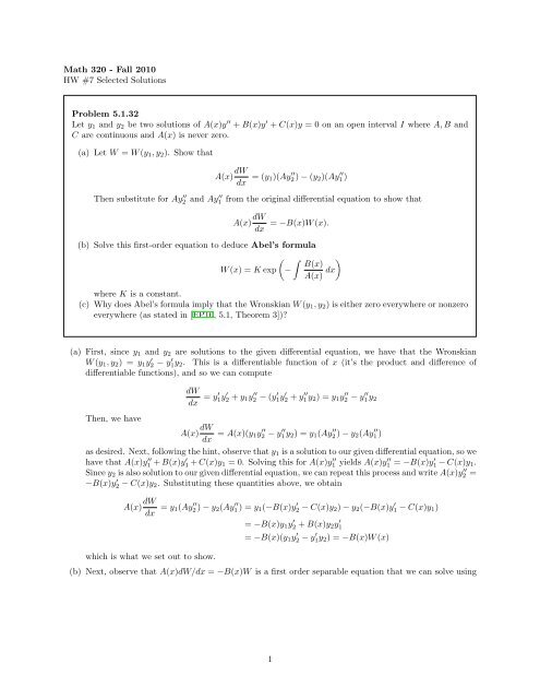
Let y1 and y2 be two solutions of A(x)y ′′ + B(x)y ′ + C(x)y = 0 on an open interval I where A, B and
C are continuous and A(x) is never zero.
(a) Let W = W (y1, y2). Show that
A(x) dW
dx
= (y1)(Ay ′′
2 ) − (y2)(Ay ′′
1 )
Then substitute for Ay ′′
2 and Ay ′′
1 from the original differential equation to show that
A(x) dW
dx
= −B(x)W (x).
(b) Solve this first-order equation to deduce Abel’s formula
� �
B(x)
W (x) = K exp −
A(x) dx
�
where K is a constant.
(c) Why does Abel’s formula imply that the Wronskian W (y1, y2) is either zero everywhere or nonzero
everywhere (as stated in [EP10, 5.1, Theorem 3])?
(a) First, since y1 and y2 are solutions to the given differential equation, we have that the Wronskian
W (y1, y2) = y1y ′ 2 − y ′ 1y2. This is a differentiable function of x (it’s the product and difference of
differentiable functions), and so we can compute
Then, we have
dW
dx = y′ 1y ′ 2 + y1y ′′
2 − (y ′ 1y ′ 2 + y ′′
1 y2) = y1y ′′
2 − y ′′
1 y2
A(x) dW
′′
= A(x)(y1y 2 − y
dx ′′
1 y2) = y1(Ay ′′
2 ) − y2(Ay ′′
1 )
as desired. Next, following the hint, observe that y1 is a solution to our given differential equation, so we
have that A(x)y ′′
1 + B(x)y ′ 1 + C(x)y1 = 0. Solving this for A(x)y ′′
1 yields A(x)y ′′
1 = −B(x)y ′ 1 − C(x)y1.
Since y2 is also solution to our given differential equation, we can repeat this process and write A(x)y ′′
2 =
−B(x)y ′ 2 − C(x)y2. Substituting these quantities above, we obtain
A(x) dW
dx
which is what we set out to show.
= y1(Ay ′′
2 ) − y2(Ay ′′
1 ) = y1(−B(x)y ′ 2 − C(x)y2) − y2(−B(x)y ′ 1 − C(x)y1)
= −B(x)y1y ′ 2 + B(x)y2y ′ 1
= −B(x)(y1y ′ 2 − y ′ 1y2) = −B(x)W (x)
(b) Next, observe that A(x)dW/dx = −B(x)W is a first order separable equation that we can solve using
1

our techniques from earlier in the semester.
dW −B(x)
=
W A(x) dx
� �
dW B(x)
= −
W A(x) dx
�
B(x)
ln |W | + C1 = −
A(x) dx
�
B(x)
ln |W | = − dx + C
A(x)
Now, first assume that W > 0. Then we have ln |W | = ln W , and then, taking exp of both sides, and
setting K = eC , we obtain
� �
B(x)
W = exp −
A(x) dx
�
e C � �
B(x)
= K exp −
A(x) dx
�
In this case, note that K = eC is a positive constant.
On the other hand, if W < 0, then ln |W | = ln −W , and so taking exp of both sides yields
� �
B(x)
W = −K exp −
A(x) dx
�
Now, since K = e C is positive, −K is negative. Then, we can label the value −K as the new constant
K, and obtain the same formula as above W = K exp(− � B(x)/A(x) dx), except now the constant K
is negative.
Finally, if W = 0, then we don’t need to solve a separable equation (in fact, if you look at the
separable equation above, it doesn’t make sense when W = 0 since we’re integrating 1/W ). However,
in this case, when W = 0, we can still use our formula W = K exp(− � B(x)/A(x) dx) simply by
setting K = 0.
(c) [EP10, 5.1 Theorem 3] says something quite peculiar. It claims that the Wronskian W (y1, y2) of two
solutions to a homogeneous second order linear equation is either always zero (in which case y1 and y2
are linearly dependent), or, W (y1, y2) is never zero (in which case y1 and y2 are linearly independent).
However, this seems to leave a gap - what if the Wronskian is sometimes zero, but not always zero?
The formula we proved in [part (b)] explains why this can’t happen.
� �
B(x)
W (x) = K exp −
A(x) dx
�
We know that an exponential function is never zero. Thus, the Wronskian, when it exists, is either
always non-zero (if K �= 0) or, always zero (if K = 0). There are no other possibilities, and so [EP10,
5.1 Theorem 3] makes sense.
2

Problem 5.1.51
A second-order Euler equation is one of the form
where a, b, c are constants.
ax 2 y ′′ + bxy ′ + cy = 0, (1)
(a) Show that if x > 0, then the substitution v = ln x transforms [Equation 1] into the constantcoefficient
linear equation
a d2y + (b − a)dy + cy = 0 (2)
dv2 dv
with independent variable v.
(b) If the roots r1 and r2 of the characteristic equation of [Equation 2] are real and distinct, conclude
that a general solution of the Euler equation in [Equation 1] is y(x) = c1x r1 + c2x r2 .
Observe that [Equation 1] is a second order linear equation, but with non-constant coefficients. The point
of this problem is to transform this non-constant equation into an equation with constant coefficients that
we can easily solve.
One important observation before we get started. The y ′ and y ′′ in [Equation 1] are derivatives with
respect to x. We want to transform them into derivatives with respect to v, so we’ll have to apply the chain
rule.
(a) Note: There’s a slightly shorter way of doing this part; see the paragraph immediately
before [part b]. Since v = ln x, we have x = e v . Then, since y is a function of x, we have
y = y(x) = y(e v ), and so y is also a function of v. Thus, it makes sense to differentiate y with respect
to v, but we must use the chain rule. Recall that if y(x) = y(g(v)), the chain rule can be written
dy
dv
dy
�
� dx
= �
dx g(v) dv
Where dy
dx | g(v) simply denotes the derivative of y with respect to x evaluated at g(v). To obtain an
expression d2 y
dv 2 , we differentiate the above expression
d2y dv2 = d2y dx2 �
� dg dx
�
g(v) dv dv
dy
�
� d
+ �
dx g(v)
2x dv2 This expression follows from [Equation 3]: simply differentiate [Equation 3] with respect to v, using
the product rule, and remember to apply the chain rule when differentiating dy
�
�
dx�
.
g(v)
Returning to the problem, suppose that x = e v , and so dx/dv = d(e v )/dv = e v . Then, y(x) = y(e v ),
and so applying the chain rule above, we have
dy dy
�
� dx
= �
dv dx ev dv
= dy
�
�
� e
dx ev v
d2y dv2 = d2y dx2 �
� de
�
ev v dx dy
�
� d
+ �
dv dv dx ev 2x dv2 = d2y dx2 �
�
�
ev eve v + dy
�
� de
�
dx ev v
dv
= d2y dx2 �
�
� e
ev 2v + dy
�
�
� e
dx ev v
3
(3)

Now, we wish to show that a d2y dv2 + (b − a) dy
dv + cy = 0, so we simply substitute in the expressions we’ve
computed for d 2 y/dv 2 and dy/dv.
a d2 � 2 y
d y
+ (b − a)dy + cy = a
dv2 dv dx2 �
�
� e
ev 2v + dy
�
�
� e
dx ev v
� �
dy
�
�
+ (b − a) � e
dx ev v
�
+ cy
= a d2y dx2 �
�
� e
ev 2v + b dy
�
�
�
dx ev = a d2y dx2 �
�
� x
x
2 + b dy
�
�
� x + cy
dx x
= ay ′′ x 2 + by ′ x + cy
= 0
e v + cy now, recall that x = e v
We obtain the third from last line, since d 2 y/dx 2 |x is simply the second derivative of y with respect to
x evaluated at x - in other words, our good old y ′′ , and similarly dy/dx|x is simply y ′ . The fact that
the last line is 0 is simply because y is a solution to the original [Equation 1].
Alternative: We can get the same derivation as above, going the other way, which has a little
clearer notation. Suppose that y(v) is a function such that y(ln x) is a solution to [Equation 1]. We
wish to show that ay ′′ (v) + (b − a)y ′ (v) + cy(v) = 0. To start off, note that (y(ln x)) ′ = y ′ (ln x)(1/x)
and (y(ln x)) ′′ = y ′′ (ln x)(1/x 2 ) + y ′ (ln x)(−1/x 2 ). Then, we have the following:
0 = ax 2 (y(ln x)) ′′ + bx(y(ln x)) ′ + cy(ln x)
= ax 2 (y ′′ (ln x)(1/x 2 ) − y ′ (ln x)(1/x 2 )) + bxy ′ (ln x)(1/x) + cy(ln x)
= ay ′′ (ln x) − ay ′ (ln x) + by ′ (ln x) + cy(ln x)
= ay ′′ (ln x) + (b − a)y ′ (ln x) + cy(ln x)
= ay ′′ (v) + (b − a)y ′ (v) + cy(v)
(b) After transforming [Equation 1] to [Equation 2] we obtain a second order linear equation with constant
coefficients. Thus, we can solve [Equation 2] simply by finding roots of the characteristic equation
ar 2 + (b − a)r + c = 0. Suppose that we’re in a situation where this characteristic equation has distinct
real roots r1 and r2. Then we know that a general solution to [Equation 2] is given by y = c1e r1v +c2e r2v
(note that the independent variable here is v, since [Equation 2] has independent variable v).
But since v = ln x, by substitution we have that
y = c1e r1v + c2e r2v = c1e r1 ln x + c2e r2 ln x = c1x r1 + c2x r2
is a solution to [Equation 1], which is what we set out to show.
4

Problem (HW 7, Problem 2)
Given one solution y1(x) to the ODE: (i) verify that y1(x) is a solution to the given ODE, and (ii) use
the method of Reduction of Order to find the general solution:
x 2 y ′′ − 4xy ′ + 6y = 0, x > 0, y1 = x 2
4x 2 y ′′ − 4xy ′ + 3y = 0, x > 0, y1 = x 1/2
x 2 y ′′ + xy ′ + y = 0, x > 0, y1 = cos(ln(x))
For these problems we’ll use the following fact from reduction of order: If y1 is a solution to a second order
linear differential equation y ′′ + p(x)y ′ + q(x)y = 0, then we can obtain the general solution yg = vy1, where
the function v satisfies the differential equation v ′′ + v ′ (2y ′ 1 + y1p)/y1 = 0
(a) We have y ′ 1 = 2x and y ′′
1 = 2, so substituting we have x 2 2 − 4x(2x) + 6x 2 = 0, and so indeed y1
is a solution. To find the general solution, we’ll use reduction of order. First, our given equation in
standard form is y ′′ − (4/x)y ′ + (6/x 2 )y = 0. Then, we must find the unknown function v that satisfies
v ′′ + v ′ (2y ′ 1 + y1p)/y1 = 0. Substituting, we wish to solve the differential equation
v ′′ + v ′
� �
2 −4 4x + x x
x2 = v ′′ = 0
This equation is easy to solve: Integrating twice yields v = c1x + c2, and so our general solution is
given by y = y1v = x 2 (c1x + c2) = c1x 3 + c2x 2 .
(b) Proceeding exactly as before, we have y ′ 1 = (1/2)x−1/2 and y ′′
1 = (−1/4)x−3/2 , and then 4x2 (−1/4)x−3/2− 4x(1/2)x−1/2 +3x1/2 = −x1/2−2x1/2 +3x1/2 = 0, and so y1 is indeed a solution. To find the general solution,
we proceed with reduction of order with the standard form equation y ′′ −(1/x)y ′ +(3/(4x2 ))y = 0
� �
−1/2 1/2 x + x (−1/x)
v ′′ + v ′
x 1/2
= v ′′ = 0
Once again, we simply have to solve v ′′ = 0, and so integrating twice yields v = c1x + c2. Then, our
general solution is given by y = vy1 = c1x 3/2 + c2x 1/2 .
(c) We first verify that y1 is indeed a solution. We have y ′ 1 = − sin(ln(x))(1/x) and y ′′
1 = −(cos(ln(x)))(1/x 2 )−
sin(ln(x))(−1/x 2 ). Then, substituting, we have
x 2 (−(cos(ln(x)))(1/x 2 )− sin(ln(x))(−1/x 2 )) + x(− sin(ln(x))(1/x)) + cos(ln(x))
= − cos(ln x) + sin(ln x) − sin(ln x) + cos(ln x)
= 0,
and so y1 is a solution to our equation. In standard form our equation is given by y ′′ +y ′ /x+y/x 2 = 0.
To find the general solution, we must find the function v that satisfies
v ′′ ′ (2(− sin(ln x)(1/x)) + cos(ln x)(1/x))
+ v = v
cos(ln x)
′′ ′ cos(ln x) − 2 sin(ln x)
+ v = 0
x cos(ln x)
If we set w = v ′ , then this is a first order linear equation, so we can apply our techniques from earlier
5

in the semester to solve it. First, let’s compute the integrating factor
�� �
cos(ln x) − 2 sin(ln x)
µ(x) = exp
dx u = ln x, du = 1/xdx
x cos(ln x)
�� �
cos u − 2 sin u
= exp
du
cos u
= exp [u + 2 ln | cos u|]
= e u ln | cos u|2
e = e u (cos u) 2 = e ln x (cos(ln x)) 2 = x(cos(ln x)) 2
Observe that we’re justified in removing our absolute values since, for any x, |x| 2 = x 2 . Proceeding
further with the integrating factor method, we have
d
dx (v′ x(cos(ln x)) 2 ) = 0
v ′ =
c1
x(cos(ln x)) 2
Now, to find v we simply integrate once more
�
c1
v =
dx
x(cos(ln x)) 2
�
c1
v =
cos
u = ln x, du = 1/xdx
2 u du
�
v = c1 sec 2 u du
v = c1 tan u + c2
v = c1 tan(ln x) + c2
Then, we have that the general solution is given by y = vy1 = c1 tan(ln x) cos(ln x) + c2 cos(ln x) =
c1 sin(ln x) + c2 cos(ln x).
References
[EP10] C. Henry Edwards and David E. Penney. Differential Equations & Linear Algebra. Prentice Hall,
Third edition, 2010.
6