Molekylmodellering med Chem3D - IFM

Molekylmodellering med Chem3D
Inledning
SS/01-05-05
Det finns ett antal förekommande beräkningsmetoder för att studera molekylers
tredimensionella struktur med datorer. Dels finns molekylmekanik metoder (MM) där
klassiska fysiklagar används som beräkningsgrund, dvs man tar främst hänsyn till
atomkärnorna och till mindre del elektronstrukturen. Dels finns kvantmekaniska metoder
(QMM) som utgår från Schrödinger ekvationen och molekylens elektronstruktur. QMM
indelas vidare i s.k. semi-empiriska och ab initio metoder. De senare metoderna bygger
mindre på experimentella data och kräver mer "datakraft" och lämpar sig därför mer för
molekyler med mindre än ≈ 100 atomer.
MM (Molecular Mechanics) lämpar sig dock för större molekylmassor (t.ex. enzymer) och
bygger till stor del på experimentella data, såsom bindningsavstånd, vinklar mm.
Energiminimering används för att minimera alla interaktioner i en molekyl så att den
stabilaste (lägst energi) strukturen antas. Molekyl dynamik (MD) där atomerna sätts i rörelse
så att de fritt får interagera med andra atomer och inta ett jämviktsläge. Om man enbart
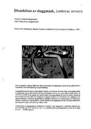
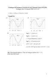
använder sig av MM är det stor risk att strukturen hamnar i ett lokalt minimum (se figur). Om
man startar med en struktur i energidiagrammmet kan den hamna i någon av de högre
energidalarna.. Det skulle inte vara den mest stabila strukturen för denna molekyl utan
molekylen skulle fastna i ett s.k. lokalt minimum. Det kan undvikas om man låter molekylen
anta en annan utgångsstruktur eller att använda MD (nedre figuren). Molekylen tillåts inta en
annan utgångspunkt eller kan att vandra utefrer den streckade linjen med hög energi och leta
upp det globala energiminimat som finns i lägsta energidalen. Det kan vara svårt att veta om
man nått det globala minimat efter enbart en energiminimering.
Energy
MIN
A
MD
B
C

Laborationsförsök
I datalaborationerna är det tänkt att laboranten ska sätta sig in i programmen ChemDrawPro
(ritprogram) och Chem3D (modelleringsprogram) genom att rita upp någon molekyl i
ChemDraw överföra denna i Chem3D samt pröva några av de olika möjligheter som
programmet medger. Främst kommer energiminimering användas men även molekyldynamik..
Minimeringsberäkningarna görs i vakuum och blir därför inte helt tillförlitliga, men
i jämförelse med opolära lösningsmedel blir dock skillnaderna små.
Följande moment avses ingå under labkursen:
1. Rita 2-dimensionella strukturer av organisk komplicerade stereostrukturer i
ritprogrammet Chem Draw.
2. Överföra strukturer från Chem Draw eller rita strukturer direkt i Chem 3D för att
visualisera strukturer tredimensionellt. (obs kontrollera att inte stereokemi ändrats!)
3. Energi minimera uppritade strukturer. Modifiera konformationer för att påvisa lokala
minima och globala minima. Ur olika värden påvisa vilka effekter som bidrar till en
molekyls totala energi.
4. Mäta bindningavstånd och vinklar mellan atomerna från modellerad molekyl.
5. Korrelera bindningsvinklar mellan väten till kopplingskonstanters storlek från
upptagna NMR spektra.
Programmen är relativt användarvänliga och enkla att förstå, men till er hjälp finns pärmar
med ledning och tutorials för de båda programmen. Framifrån : ChemDraw (ritprogrammet)
och Bakfrån Chem3D (minimeringsprogrammet). Vidare lärarhjälp.
Uppgifter:
A. Rita i ChemDraw en komplicerad molekylstruktur tvådimensionellt så att alla stereogena
kols bindningar har rätt riktning tredimensionellt.
Välj två av dessa: sackaros, adenine, estradiol, vitamin A, morfin. Rita ut strukturen för
redovisning.
Överför strukturen till Chem 3D (klipp och klistra) och se molekylen tredimmensionellt.
Energiminimerea och välj lämpligt sätt att presentera molekylen utskriven (ej färg).
B. Med Chem 3D energiminimeras ett lämligt substituerat cyklohexan-derivat. Olika
konformationer jämförs t.ex. Twisted-boat och Chair. Jämför och kommentera de olika
konformationernas värden. Diskuteras gärna med andra gruppers resultat på liknande
isomera cyklohexan-derivat. Vilken av nedan strukturer tror ni har mest stabil och minst
stabil stolform ? Tag fram ert resultat och jämför med andra gruppers resultat.
1. Grp A+D: cis- och trans-1,2-dimetylcyklohexan
2. Grp B+E : cis- och trans-1,3-dimetylcyklohexan
3. Grp C+F: cis- och trans-1,4-dimetylcyklohexan
Rita upp strukturen. Minimera strukturen och anteckna erhållna värden på stretch, bend,
stretch-bend, torsion, non-1,4-vdW, 1,4-vdW, dipol/dipol och total energi.
Chair-konformationen har generellt lägst energi. Flytta om några kol och se om ni kan hitta
olika lokala minima. Ett sådant som man ofta kan hitta är twist-boat konformation
Vid minimeringarna kan man använda de utgångsvärden som är angivna för MM2: minimize
energy.

Några tips (Chem3D)
• Det är enklare att se strukturen om man gömmer alla väten (Tools: Show H´s)
• Vill man invertera ett stereocenter kan man göra detta med genom att markera atomen och
använda Tools: Invert. Vid överföring från ChemDraw till Chem3D måste stereocenter
kontrolleras, eftersom det ibland händer att en godtycklig stereokemi väljs.
• Under View: Preferences kan man ändra utseendet på molekylen (ball and sticks är att föredra!)
C: Molekylmodellering kan användas för att förut se stereoselektivitet. Föreslå från den
tvådimensionella strukturen nedan hur alla tre dubbelbindningarna kommer att
epoxideras med MCPBA (meta-chlorperbenzoic acid). Gör den tredmensionella
strukturen, energiminimera och avgör om det förra antagandet stämmer då du ser den
tredimensionellt. Redovisa den troliga produkten tvådimensionellt i ChemDraw.
O
O
MCPBA
Vid senare laborationer:
Ett senare mål är att göra en konformationsminimering på organiska föreningar från
laborationer, som strukturidentifierats med NMR. Erhållna kopplingskonstanter från NMR
spektrat kan ur Kaplus formeln (se spektroskopibokem) ge vinklar som jämförs med
bindningsvinklar ur den med Chem3D byggda och energiminimerade strukturen.
Redovisning:
A. Namn på vald struktur, två-dimensionell struktur samt tre-dimensionellt minimerad
struktur.
B. .För resp. cis- och trans-struktur redovisas tredimensionell minimerad struktur för chair,
twisted-boat och ev. boat-form, och data för resp. konformation. Även kort diskussion
kring struktur, konformation och erhållna energivärden. Via egna funderingar och andra
gruppers resultat, vilken struktur är stabilast ? Stämmer egna antaganden med resultatet ?
C. Uppritad utgångsstruktur och den trriepoxiderade strukturen där epoxidernas
tredimensionella orientering inritas på utgångsstrukturen. Minimerat totalvärde och
tredimensionell struktur på utgångsstruktur och produkt redovisas även.

COMPUTATIONAL CHEMISTRY
Computational chemistry extends beyond thetraditional boundaries separating chemistry from physics,
biology, and computer science. Though pioneering work in this area predates by decades the 1980
debut of its namesake journal, the Journal of Computational Chemistry, computational chemistry, as a
distinct area of research, is relatively new. It allows the exploration of molecules through the use of a
computer in cases when an actual laboratory investigation may be inappropriate, impractical, or
impossible. As an adjunct to experimental chemistry, its significance continues to be enhanced by
explosive increases in computer speed and power.
Aspects of computational chemistry include molecular modeling, computational methods, and
Computer Aided Molecular Design (CAMD), as well as chemical databases, and organic
synthesis design.
While a number of different definitions have been proposed, the definition offered by Lipkowitz and
Boyd of computational chemistry as “those aspects of chemical research that are expedited or rendered
practical by computers” is perhaps the most inclusive.
Molecular modeling, while often taken to include computational methods, can be thought of as the
rendering of a 2D or 3D model of a molecule‘s structure and properties. Computational methods, on
the other hand, calculate the structure and property data necessary to render the model. Within a
modeling program, such as Chem3D, computational methods are referred to as computation engines,
while geometry engines and graphics engines render the model.
Only within the past few years has it become possible to perform genuinely useful molecular
computations with a desktop personal computer. Chem3D supports a number of powerful
computational chemistry methods on the desktop in addition to its extensive visualization options. The
rest of this chapter will provide an introduction to the computational methods available through
Chem3D.
COMPUTATIONAL METHODS OVERVIEW
Computational chemistry encompasses a variety of mathematical methods which fall into two broad
categories: molecular mechanics and quantum mechanics.
Molecular mechanics applies the laws of classical physics to molecular nuclei without explicit
consideration of electrons.
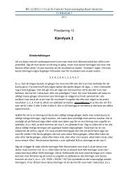
Quantum mechanics relies on the Schrödinger
equation to describe a molecule with explicit
treatment of electronic structure. Generally,
quantum mechanical methods can be
subdivided into two classes: ab initio and
semiempirical, making a total of three
generally accepted method classes, as shown
beside.
All three classes are available through Chem3D. The molecular mechanical MM2 method, and the
semiempirical Extended Hückel, MINDO/3, MNDO, MNDO-d, AM1 and PM3 methods are directly
available from within Chem3D and CS MOPAC, while ab initio methods are available through
Chem3D’s Gaussian interface. An individual computational method may also be referred to as a
theory.
Uses of Computational Methods
Computational methods calculate the potential energy surfaces of molecules. The potential energy
surface (PES) can be considered to be the embodiment of the forces of interaction among atoms in a
molecule; from the PES, structural and chemical information about a molecule can be derived. While
the methods differ in the way the surface is calculated, and in the molecular properties that can be
derived from the energy surface, they generally perform the following basic types of calculations:
• single point energy calculation, which is the energy of a given spacial arrangement of the atoms in
a model, or more precisely, the value of the PES for a given set of atomic coordinates.

• geometry optimization, which is a systematic modification of the atomic coordinates of a model
resulting in a geometry where the net forces on the structure sum to zero, or in other word, a 3dimensional
arrangement of atoms in the model representing a local energy minimum (a stable
molecular geometry to be found without crossing a conformational energy barrier).
• property calculation, which predicts certain physical and chemical properties, such as charge,
dipole moment and heat of formation. Additionally such methods may be employed to perform more
specialized functions, such as conformational searches and molecular dynamics simulations.
Choosing the Best Method
Not all types of calculations are possible for all methods, and no one method is best for all purposes.
For any given application, each method will pose advantages and disadvantages. Choice of method
will depend on a number of factors, including the nature of the molecule, the type of information
sought, the availability of applicable experimentally determined parameters (as required by some
methods), as well as more practical matters of available computer resources and time. The three most
important of the these criteria are:
1. Model size: The size of a model can be a serious limiting factor for a particular method. In general,
the limiting number of atoms in a molecule increases by approximately one order of magnitude
between method classes from ab initio to molecular mechanics. Accordingly ab initio is limited to tens
of atoms, semiempirical to hundreds, and molecular mechanics to thousands.
2. Parameter Availability: Some methods depend on experimentally determined parameters to
perform computations. If the model contains atoms for which the parameters of a particular method
have not been derived, that method may produce invalid predictions. Molecular mechanics, for
instance, relies on parameters to define a force-field. Any particular force-field is only applicable to
the limited class of molecules for which it is parametrized.
3. Computer resources: Requirements increase in the following manner relative to the size of the
model for each of the methods.
Ab initio : The time required for performing computations increases on the order of N 4 , where N is the
number of atoms in the model.
Semiempirical: The time required for computation increases as N 3 or N 2 , where N is the number of
atoms in the model.
MM2: The time required for performing computations increases as N 2 , where N is the number of
atoms.
In general, molecular mechanical methods are computationally less expensive than quantum
mechanical methods. The suitability of each general method for particular applications can be
summarized as follows.
Molecular Mechanics Methods Applications
Summary
Molecular mechanics, in Chem3D, can successfully be applied to:
• Systems containing thousands of atoms.
• Organic, oligonucleotides, peptides, and saccharides.
• Gas phase only (for MM2) Useful techniques available using MM2 methods include:
• Energy Minimization for locating stable conformations.
• Single point energy calculations for comparing conformations of the same molecule.
• Searching conformational space by varying a single dihedral angle.
• Studying molecular motion using Molecular Dynamics.
Quantum Mechanical Methods Applications
Summary
The semiempirical methods available in Chem3D and CS MOPAC can be successfully applied to:
• Systems containing up to 60 heavy atoms and 120 total atoms (in CS MOPAC).
• Organic, organometallics, and small oligomers (peptide, nucleotide, saccharide).
• Gas phase or implicit solvent environment.
• Ground, transition, and excited states.
Ab initio methods (available through the Gaussian interface) can be successfully applied to:

• Systems containing up to ca. 30 atoms.
• Organic, organometallics, and molecular fragments (e.g. catalytic components of an enzyme).
• Gas or implicit solvent environment.
• Study ground, transition, and excited states (certain methods).
Useful information determined by quantum mechanical methods includes:
• Molecular orbital energies, and coefficients.
• Heat of Formation for evaluating conformational energies.
• Partial atomic charges calculated from the molecular orbital coefficients.
• Electrostatic potential.
• Dipole moment.
• Transition-state geometries and energies.
• Bond dissociation energies.
Summary of Method types:

Potential Energy Surfaces
A potential energy surface (PES) can describe:
• either a molecule or ensemble of molecules having constant atom composition (ethane, for example),
or a system where a chemical reaction occurs.
• relative energies for conformers (e.g. eclipsed and staggered forms of ethane).
NOTE: It is important to keep in mind that different potential energy surfaces are generated for:
• molecules having different atomic composition (ethane and chloroethane).
• molecules in excited states than for the same molecules in their ground states.
• molecules with identical atomic composition but with different bonding patterns, such as
propylene and cyclopropane.
Points of interest on a Potential Energy surface.
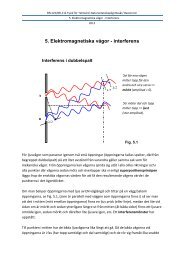
The true representation of a model’s potential
energy surface is a multi-dimensional surface
whose dimensionality increases with the
number of independent variables. Since each
atom has three
independent variables (x, y, z coordinates),
visualizing a surface for a many-atom model is
impossible. However, we can generalize this
problem by examining any 2 independent
variables, such asthe x and y coordinates of an
atom, as shown below:
Potential Energy Surface Representing 2 Variables
The main areas of interest on a potential energy surface are the extrema indicated above by arrows.
The most stable conformation appears at the extremum where the energy is lowest. This extremum is
called the global minimum. There is only one global minimum for a molecule; however, for all but
the simplest molecules, there are additional low energy extrema, termed local minima. Minima are
defined by regions of the PES where a change in geometry.
The last extremum of interest is at a point between two low energy extrema and is termed a saddle
point. The saddle point is defined as a point on the potential energy surface at which there is an
increase in energy in all directions except one, and for which the slope (first derivative) of the surface
is zero.
NOTE: At the energy minimum, the energy is not zero; the first derivative (gradient) of the energy with
respect to geometry is zero.
All the minima on a potential energy surface of a molecule represent stable stationery points where the
forces on atoms sum to zero. The global minimum represents the most stable conformation; the local
minima, less stable conformations; and the saddle points represent transition conformations between
minima.
Single Point Energy Calculations
Single point energy calculations can be used tocalculate properties of the current geometry of a model.
The values of these properties are dependent on where the model currently lies on the potential
surface. Further:
1. A single point energy calculation at a global minimum provides information about the model
in its most stable conformation.
2. A single point calculation at a local minimum provides information about the model in one of
many stable conformations.

3. A single point calculation at a saddle point provides information about the transition state of
the model.
4. A single point energy calculation at any other point on the potential energy surface provides
information about that particular geometry, not a stable conformation or transition state.
Single point energy calculations may be performed either before or after performing an optimization,
though.
NOTE: Since different methods rely on different assumptions about a given molecule, values derived
from different methods should NOT be compared!
Geometry Optimization
Geometry optimization is a technique used for locating a stable conformation of a model. As a general
rule, this should be performed before performing additional computations or analyses of a model.
Locating global and local energy minima is often accomplished through energy minimization;
locating a saddle point is referred to as optimizing to a transition state.
The ability of a geometry optimization to converge to a minimum will depend on the starting
geometry, the potential energy function used, and the settings for a minimum acceptable gradient
between steps (convergence criteria).
Geometry optimizations are iterative and begin at some starting geometry. First, the single point
energy calculation is performed on the starting geometry. Then the coordinates for some subset of
atoms are changed and another single point energy calculation is performed to determine the energy of
that new conformation. The first or second derivative of the energy (depending on the method) with
respect to the atomic coordinates then determines how large and in what direction the next increment
of geometry change should be. Then the change is made.
Following the incremental change, the energy and energy derivatives are again determined and the
process continues until convergence is achieved, at which point the minimization process terminates.
The figure below illustrates some concepts of
minimization. For simplicity, this plot shows a
single independent variable plotted in two
dimensions.
1. The starting geometry of the model will determine which minimum is reached. For instance, starting
at (b), minimization will result in geometry (a), which is the global minimum. However, starting at (d)
will lead to geometry (f), which is a local minimum.
2. The proximity to a minimum, but not a particular minimum, can be controlled by specifying a
minimum gradient that should be reached. Geometry (f), rather than geometry (e), can be reached by
decreasing the value of the gradient where the calculation ends.
3. Often, if a convergence criterion (energy gradient) is too lax, a first-derivative minimization can
result in a geometry that is near a saddle point. This occurs because the value of the energy gradient
near a saddle point, as near a minimum, is very small. For example, at point (c), the derivative of the
energy is 0, and as far as the minimizer is concerned, point (c) is a minimum. First derivative
minimizers cannot, as a rule, surmount saddle points to reach another minimum.
There are several steps which may be taken to ensure that a minimization has not resulted in a saddle
point.
1. The geometry can be altered slightly and another minimization performed. The new starting
geometry might result in either (a), or (f) in a case where the original one led to (c).
2. The Dihedral Driver (Macintosh only. See Chapter 10, MM2 Computations, for more information.)
can be employed to search the conformational space of the model.

3. A molecular dynamics simulation can be run, which will allow small potential energy barrier to be
crossed. After completing the molecular dynamics simulation, individual geometries can then be
minimized and analyzed. (For further information, see Chapter 10, MM2 Computations.)
Property Calculations
From the PES, many molecular properties can be calculated. The properties which can be calculated
with the computational methods available through Chem3D include: steric energy, heat of formation,
dipole moment, charge density, COSMO solvation in water, electrostatic potential, electron spin
density, hyperfine coupling constants, atomic charges, polarizability, and others, such as IR vibrational
frequencies. These properties are discussed in more detail in the following chapters.
MOLECULAR MECHANICS THEORY IN BRIEF
Molecular mechanics describes the energy of a molecule in terms of a set of classically derived energy
functions. The potential energy functions and the parameters used for their evaluation are known as a
“force-field”. Molecular mechanical methods are based on the following principles:
4. Nuclei and electrons are lumped together and treated as unified atom-like particles.
5. Atom-like particles are typically treated as spheres.
6. Bonds between particles are viewed as harmonic
7. Non-bonded interactions between these particles are treated using potential functions
derived using classical mechanics.
8. Individual potential functions are used to describe the different interactions: bond
stretching, angle bending, and torsional (bond twisting) energies, and through-space (nonbonded)
interactions.
9. Potential energy functions rely on empirically derived parameters (force constants,
equilibrium values) that describe the interactions between sets of atoms.
10. The sum of interactions determine the spatial distribution (conformation) of atom-like
particles.
11. Molecular mechanical energies have no meaning as absolute quantities. They can only be
used to compare relative steric energy (strain) between two or more conformations of the
same molecule.
12.
The Force-Field
Molecular mechanics typically treats atoms as spheres, and bonds as springs. The mathematics of
spring deformation (Hooke’s Law) is used to describe the ability of bonds to stretch, bend, and twist.
Non-bonded atoms (greater than two bonds apart) interact through van der Waals attraction, steric
repulsion, and electrostatic attraction/repulsion. These properties are easiest to describe
mathematically when atoms are considered as spheres of characteristic radii.
The total potential energy, E, of a molecule can be described by the following summation of
interactions.
Energy = Stretching Energy + Bending Energy + Torsion Energy + Non-Bonded Interaction Energy
The first three terms, given as a, b, and c below, are the so-called bonded interactions. In general, these
bonding interactions can be viewed as a strain energy imposed by a model moving from some ideal
zero strain conformation. The last term, which represents the non-bonded interactions, includes the
two interactions shown below as e and f. The total potential energy, then, can be described by the
following relationships between atoms (with numbers indicating the relative positions of the
atoms):
a. Bond Stretching: (1-2) bond stretching between directly bonded atoms
b. Angle Bending: (1-3) angle bending between atoms that are geminal to each other.
c. Torsion Energy: (1-4) torsional angle rotation between atoms that are vicinal to each other.
d. Repulsion for atoms that are too close and attraction at long range from dispersion forces (van
der Waals interaction).
e. Interactions from charges, dipoles, quadrupoles (electrostatic interactions).

The picture below illustrates the major
interactions.
Many different kinds of force-fields have been developed over the years. Some include additional
energy terms that describe other kinds of deformations, such as the coupling between bending and
stretching in adjacent bonds, in order to improve the accuracy of the mechanical model.
The reliability of a molecular mechanical force-field depends on the parameters and the potential
energy functions used to describe the total energy of a model. Parameters must be optimized for a
particular set of potential energy functions, and thus are not easily transferable to other force fields.
MM2
Chem3D uses a modified version of Allinger’s MM2 force field. See Appendix E, MM2, for additional
references for MM2.
NOTE: The principal additions to Allinger’s MM2 force field are:
C. a charge-dipole interaction term.
D. a quartic stretching term.
E. cutoffs for electrostatic and van der Waals terms with 5th order polynomial switching function.
F. automatic pi system calculations when necessary.
G. Torsional and non-bonded constraints.
CS Chem3D stores the parameters used for each of the terms in the potential energy function in tables.
These tables are controlled by the Table Editor application, which allows viewing and editing of the
parameters. Descriptions of the information within each parameter table is further described in the online
help file under the topic “Fields in Parameter Tables”.
Each parameter is classified by a Quality number. This number indicates the reliability of the data. The
quality ranges from 4, where the data are derived completely from experimental data (or ab initio
data), to 1, where the data are guessed by Chem3D.
The parameter table “MM2 Constants” contains many adjustable parameters that correct for failings of
many of the potential functions in outlying situations.
The terms in the MM2 potential energy function are
• Bond Stretching Energy
• Angle Bending Energy
• Torsion Energy
• Non-Bonded Energy
• Electrostatic Energy