
Create successful ePaper yourself
Turn your PDF publications into a flip-book with our unique Google optimized e-Paper software.
ADVANCED<br />
DATA<br />
STRUCTURE<br />
NOTES<br />
(MTCSE<br />
110)<br />
Prepared By :<br />
Er. Harvinder Singh<br />
Assist Prof, C.S.E<br />
H.C.T.M (Kaithal)<br />
JULY 25, 2011<br />
2011
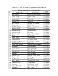
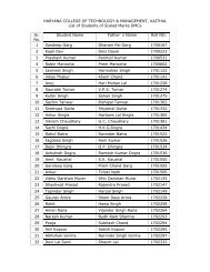
LECTURE NOTES OF ADVANCED DATA STRUCTURE (MT-CSE 110)<br />
Introduction to sorting<br />
Sorting Techniques<br />
Sorting is a process in which arranging of data is done in some given sequence<br />
increasing or decreasing order . Searching for an element will be more efficient in<br />
an array<br />
Categorization:<br />
internal sorting external sorting<br />
Arranigng the no’s within the sorting of no. from<br />
the array only which is in external file by<br />
reading it primary memory from secondary memory<br />
Why we do sorting?<br />
Commonly encountered programming task in computing.<br />
Examples of sorting:<br />
<strong>1.</strong> List containing exam scores sorted from Lowest to Highest or from<br />
Highest to Lowest<br />
2. List containing words that were misspelled and be listed in<br />
alphabetical order.<br />
3. List of student records and sorted by student number or<br />
alphabetically by first or last name.<br />
Prepared By :<br />
Er. Harvinder Singh<br />
Assist Prof., CSE, H.C.T.M (Kaithal) Page ‐ 2 ‐
LECTURE NOTES OF ADVANCED DATA STRUCTURE (MT-CSE 110)<br />
Algorithm for Quick Sort<br />
Quik_Sort(a,l,h)<br />
Where a = represents list of elements.<br />
l = represents the position of the first element in the list<br />
h = represents the position of the last element in the list<br />
<strong>1.</strong> [Initially]<br />
low =l<br />
high =h<br />
key = a[(l + h)/2] [Middle element of the list]<br />
2. Repeat through step 7 while (low
LECTURE NOTES OF ADVANCED DATA STRUCTURE (MT-CSE 110)<br />
<strong>1.</strong>INITIAL STEP‐ FIRST PARTITION<br />
2.SORT LEFT PART IN SAME WAY<br />
Prepared By :<br />
Er. Harvinder Singh<br />
Assist Prof., CSE, H.C.T.M (Kaithal) Page ‐ 4 ‐
LECTURE NOTES OF ADVANCED DATA STRUCTURE (MT-CSE 110)<br />
INTRODUCTION OF QUICK SORT<br />
Quick sort is a divide‐and‐conquer style algorithm. A divide‐and‐conquer<br />
algorithm solves a given problem by splitting it into two or more smaller sub<br />
problems, recursively solving each of the sub problems, and then combining the<br />
solutions to the smaller problems to obtain a solution to the original one.<br />
To sort the sequence S={S1,S2,S3,…………,Sn}, quick sort performs the following<br />
steps:<br />
<strong>1.</strong> Select one of the elements of S. The selected element, p, is<br />
called the pivot.<br />
2. Remove p from S and then partition the remaining<br />
elements of S into two distinct sequences, L and G, such<br />
that every element in L is less than or equal to the pivot<br />
and every element in G is greater than or equal to the<br />
pivot. In general, both L and G are unsorted.<br />
3. Rearrange the elements of the sequence as follows:<br />
Notice that the pivot is now in the position in which it belongs in the<br />
sorted sequence, since all the elements to the left of the pivot are less<br />
than or equal to the pivot and all the elements to the right are greater<br />
than or equal to it.<br />
4. Recursively quick sort the unsorted sequences L and G.<br />
The first step of the algorithm is a crucial one. We have not specified how to<br />
select the pivot. Fortunately, the sorting algorithm works no matter which<br />
element is chosen to be the pivot. However, the pivot selection affects directly<br />
the running time of the algorithm. If we choose poorly the running time will be<br />
poor.<br />
Figure illustrates the detailed operation of quick sort as it sorts the sequence<br />
{3,1,4,1,5,9,2,6,5,4}. To begin the sort, we select a pivot. In this example, the<br />
Prepared By :<br />
Er. Harvinder Singh<br />
Assist Prof., CSE, H.C.T.M (Kaithal) Page ‐ 5 ‐
LECTURE NOTES OF ADVANCED DATA STRUCTURE (MT-CSE 110)<br />
value 4 in the last array position is chosen. Next, the remaining elements are<br />
partitioned into two sequences, one which contains values less than or equal to<br />
4 (L={3,1,2,1}) and one which contains values greater than or equal to 4<br />
(G={5,9,4,6,5}). Notice that the partitioning is accomplished by exchanging<br />
elements. This is why quick sort is considered to be an exchange sort.<br />
Prepared By :<br />
Er. Harvinder Singh<br />
Assist Prof., CSE, H.C.T.M (Kaithal) Page ‐ 6 ‐
LECTURE NOTES OF ADVANCED DATA STRUCTURE (MT-CSE 110)<br />
Algorithm for Bucket Sort<br />
Bucket_Sort(A,N)<br />
Where A = Linear Array,N = Number of elements in linear array, A.<br />
<strong>1.</strong> Find the largest element of the array.<br />
2. Find the total number of digits num in the largest digit<br />
Set digit = num<br />
3. Repeat step 4 , 5 for pass = 1 to num<br />
4. Initialize buckets<br />
For i=1 to (n‐1)<br />
Set num = obtain digit number pass of a[i]<br />
Put a[i] in bucket number digit<br />
[end of for loop]<br />
5. Calculate all number from the bucket in order.<br />
6. Exit<br />
Radix/Bucket Sort Theory<br />
Radix Sort is one of the linear sorting algorithms for integers. This sorting<br />
technique is also known as Bucket Sort or Pocket Sort. It functions by sorting the<br />
input numbers on each digit, for each of the digits in the numbers. However, the<br />
process adopted by this sort method is somewhat counterintuitive, in the sense<br />
that the numbers are sorted on the least‐significant digit first, followed by the<br />
second‐least significant digit and so on till the most significant digit.<br />
To appreciate Radix Sort, consider the following analogy: Suppose that we wish<br />
to sort a deck of 52 playing cards (the different suits can be given suitable<br />
values, for example 1 for Diamonds, 2 for Clubs, 3 for Hearts and 4 for Spades).<br />
The 'natural' thing to do would be to first sort the cards according to suits, then<br />
sort each of the four seperate piles, and finally combine the four in order. This<br />
Prepared By :<br />
Er. Harvinder Singh<br />
Assist Prof., CSE, H.C.T.M (Kaithal) Page ‐ 7 ‐
LECTURE NOTES OF ADVANCED DATA STRUCTURE (MT-CSE 110)<br />
approach, however, has an inherent disadvantage. When each of the piles is<br />
being sorted, the other piles have to be kept aside and kept track of. If, instead,<br />
we follow the 'counterintuitive' aproach of first sorting the cards by value, this<br />
problem is eliminated. After the first step, the four seperate piles are combined<br />
in order and then sorted by suit. If a stable sorting algorithm (i.e. one which<br />
resolves a tie by keeping the number obtained first in the input as the first in<br />
the output) it can be easily seen that correct final results are obtained.<br />
As has been mentioned, the sorting of numbers proceeds by sorting the<br />
least significant to most significant digit. For sorting each of these digit<br />
groups, a stable sorting algorithm is needed. Also, the elements in this<br />
group to be sorted are in the fixed range of 0 to 9.<br />
Example:<br />
To illustrate the bucket sort method, consider following list of numbers:<br />
121, 70, 965, 432, 12, 577, 683<br />
Solution:<br />
Pass 1:<br />
121<br />
70<br />
965<br />
432<br />
12<br />
577 12<br />
683 70 121 432 683 965 577<br />
Input 0 1 2 3 4 5 6 7 8 9<br />
Pass 2:<br />
Prepared By :<br />
Er. Harvinder Singh<br />
Assist Prof., CSE, H.C.T.M (Kaithal) Page ‐ 8 ‐
70<br />
121<br />
432<br />
12<br />
638<br />
LECTURE NOTES OF ADVANCED DATA STRUCTURE (MT-CSE 110)<br />
965 70<br />
577 12 121 432 965 577 683<br />
Input 0 1 2 3 4 5 6 7 8 9<br />
Pass 3:<br />
70<br />
121<br />
432<br />
12<br />
638<br />
965 70<br />
577 12 121 432 577 683 965<br />
Input 0 1 2 3 4 5 6 7 8 9<br />
After pass 3, when the numbers are collected, they are in the following order<br />
Prepared By :<br />
Er. Harvinder Singh<br />
Assist Prof., CSE, H.C.T.M (Kaithal) Page ‐ 9 ‐
LECTURE NOTES OF ADVANCED DATA STRUCTURE (MT-CSE 110)<br />
12, 70, 121, 432, 577, 683, 965<br />
Thus, the numbers are sorted.<br />
Algorithm for Merge Sort<br />
Merge_Sort(A,N)<br />
Where A = Linear Array.<br />
N = Number of elements in linear array, A.<br />
<strong>1.</strong> [ Call the recursive function divide ]<br />
Call divide (A,1,N)<br />
2. [ Finished ]<br />
Exit<br />
Procedure : divide (A, first, last)<br />
This function consider the array A. first and last variables represents the index<br />
of the first and the last element of the array A, respectively. The variable mid<br />
represents the middle position of array A.<br />
<strong>1.</strong> [ divide the array recursively ]<br />
If ( first < last) then<br />
mid := (first + last )/2<br />
call divide ( A, first, mid)<br />
call divide ( A, mid+1, last)<br />
call merge ( A, first, mid, last);<br />
Prepared By :<br />
Er. Harvinder Singh<br />
Assist Prof., CSE, H.C.T.M (Kaithal) Page ‐ 10 ‐
LECTURE NOTES OF ADVANCED DATA STRUCTURE (MT-CSE 110)<br />
[ End of if statement ]<br />
2. [ Finished ]<br />
Return<br />
Procedure : merge (A, first, mid, last )<br />
Here first, mid and last represents the first, middle and last position of array A.<br />
In this procedure we use auxiliary array TEMP. The variables i, j, k are local<br />
variables.<br />
<strong>1.</strong> [ Initialise ]<br />
i = first, j = mid + 1, k = first<br />
2. [ compare elements and output the smaller in array TEMP ]<br />
Repeat while (i
LECTURE NOTES OF ADVANCED DATA STRUCTURE (MT-CSE 110)<br />
j = j + 1<br />
[ End of loop ]<br />
4. [ Copy array TEMP into array A ]<br />
Repeat for i = first to last<br />
A [i] = TEMP [i]<br />
[ End of for loop ]<br />
5. [ Finished ]<br />
Return<br />
MERGE‐SORT Theory<br />
Merging is the process of combining two sorted lists into one sorted list. For this<br />
the elements from both the sorted list are compared. The smaller of both the<br />
elements is then sorted in the third array. The sorting is complete when all the<br />
elements from both the lists are placed in the third list<br />
EXAMPLE OF MERGE‐ SORT<br />
Suppose the array A contains 12 elements as follow:<br />
85, 76, 46, 92, 30, 41,12, 19, 93, 3, 50, 11<br />
Each pass of the merge sort algorithm will start at the beginning of the array A<br />
and merge pairs of sorted subarrays as follow:<br />
Pass1: merge each pair of elements to obtain the following list of sorted<br />
pairs:<br />
76 85<br />
46 92<br />
30 41<br />
12 19<br />
Prepared By :<br />
Er. Harvinder Singh<br />
Assist Prof., CSE, H.C.T.M (Kaithal) Page ‐ 12 ‐
3 91<br />
11 50<br />
LECTURE NOTES OF ADVANCED DATA STRUCTURE (MT-CSE 110)<br />
Pass 2:merge each pair of pairs to obtain the lists of sorted elements.<br />
46 76 85 92<br />
12 19 30 41<br />
3 11 50 93<br />
Pass 3: again merge the two subarrays to get two lists.<br />
12 19 30 41 46 76 85 92<br />
3 11 50 93<br />
Pass 4: merging the above two lists, we get.<br />
3 11 12 19 30 41 46 50 76 85 92 93<br />
Prepared By :<br />
Er. Harvinder Singh<br />
Assist Prof., CSE, H.C.T.M (Kaithal) Page ‐ 13 ‐
LECTURE NOTES OF ADVANCED DATA STRUCTURE (MT-CSE 110)<br />
Algorithm for Heap Sort<br />
Create_Heap(A,N)<br />
Where A = Linear Array.<br />
N = Number of elements in linear array, A.<br />
The index variable Count controls the number of insertion. The integer variable j<br />
denotes the index of the parent of key k[i], key contains he element being<br />
inserted into an existing heap.<br />
<strong>1.</strong> [ Repeat for each element to be placed in heap ]<br />
Repeat step 2 to step 7 for Count = 2 to N<br />
2. [ Obtain child to be placed at heap level ]<br />
i = Count<br />
key = A [Count]<br />
3. [ Obtain the position of parent for his child ]<br />
j = i div 2<br />
4. [ Place the child in existing heap ]<br />
Repeat step 5 to 6 while i > 1 and key > A[ j]<br />
5. [ Move the parent down to the position of the child ]<br />
A[i] = A[j]<br />
6. [ Obtain the position of the new parent ]<br />
i = j<br />
j = i div 2<br />
if j < 1 then<br />
Prepared By :<br />
Er. Harvinder Singh<br />
Assist Prof., CSE, H.C.T.M (Kaithal) Page ‐ 14 ‐
LECTURE NOTES OF ADVANCED DATA STRUCTURE (MT-CSE 110)<br />
j = 1<br />
[ End of if statement ]<br />
[ End of step 4 loop ]<br />
7. [ Copy the child record into its proper place ]<br />
A [i] = key<br />
[ End of step 1 for loop ]<br />
8. [ Finished ]<br />
Return<br />
Algorithm : Heap_Sort ( A,N )<br />
<strong>1.</strong> [ Create the initial heap ]<br />
Call Create_Heap (A,N)<br />
2. [ Perform the sort ]<br />
Repeat step 3 to 10 for Count = N to i‐1<br />
3. [ Exchange the first element with the last unsorted element ]<br />
A [i] = A [Count]<br />
4. [ Initialise Pass]<br />
i = 1<br />
key = A[i]<br />
j = 2<br />
5. [ Obtain index of largest son ]<br />
if j+1 < Count then<br />
if A[j+1] > A[j] then<br />
j = j +1<br />
[ End of inner if statement]<br />
Prepared By :<br />
Er. Harvinder Singh<br />
Assist Prof., CSE, H.C.T.M (Kaithal) Page ‐ 15 ‐
LECTURE NOTES OF ADVANCED DATA STRUCTURE (MT-CSE 110)<br />
[ End of outer if statement]<br />
6. [ Reconstruct the new heap ]<br />
Repeat step 7 to 10 while (j key)<br />
7. [ Interchange element ]<br />
A[i] = A[j]<br />
8. [ Obtain the next left son]<br />
i = j<br />
j= 2 *i<br />
9. [ Obtain the index of next largest son ]<br />
If j+1 < Count then<br />
If A [j+1] > A[j] then<br />
j = j + 1<br />
[ End of inner if statement]<br />
Else<br />
If j > n then<br />
j = n<br />
[ End of inner if statement]<br />
[ End of outer if statement]<br />
10. [ Copy the record into its proper place ]<br />
A[i] = key<br />
1<strong>1.</strong> [ Finished ]<br />
Exit<br />
HEAP SORT Theory<br />
A Heap is a binary tree that satisfies the following properties :‐<br />
<strong>1.</strong> Heap must be a complete binary tree.<br />
2. For every node in the heap, the value stored in that node is greater than<br />
or equal to the value in each of its children. This is known as order<br />
Prepared By :<br />
Er. Harvinder Singh<br />
Assist Prof., CSE, H.C.T.M (Kaithal) Page ‐ 16 ‐
LECTURE NOTES OF ADVANCED DATA STRUCTURE (MT-CSE 110)<br />
property and a heap that satisfies this property is known as maximum<br />
heap.<br />
If the order property is such that for every node in the heap, the value stored in<br />
that node is less than or equal to the value in each of its children, then that<br />
heap is known as minimum heap.<br />
STEPS IN HEAP SORT<br />
Heap sort follows two main steps:‐<br />
Step I:‐ creation of heap<br />
Step II:‐ operation on heap<br />
CREATION OF HEAP<br />
A heap is a complete binary tree in which every node satisfies the heap<br />
condition.<br />
HEAP CONDITION<br />
A complete binary tree is said to satisfy the heap condition if the key of each<br />
node is greater than or equal to the key in its children.<br />
Thus the root node will have the largest key value<br />
OPERATION ON HEAP<br />
The steps of operations are as follows:‐<br />
Step I – Remove the root node of the heap and insert it into the sorted list from<br />
right to left.<br />
Step II‐ Replace the deleted element (root) by the last element.<br />
Prepared By :<br />
Er. Harvinder Singh<br />
Assist Prof., CSE, H.C.T.M (Kaithal) Page ‐ 17 ‐
LECTURE NOTES OF ADVANCED DATA STRUCTURE (MT-CSE 110)<br />
Step III‐Reconstruct a new heap which now consists of N‐1 elements.<br />
Repeat the steps I,II & III to get the desired sorted list.<br />
ALGORITHM FOR SELECTION SORT<br />
Selection_Sort (A,N)<br />
Here A is a linear array having N no. of elements<br />
<strong>1.</strong> Set I=LB<br />
2. Repeat steps 3,4,7 while I
LECTURE NOTES OF ADVANCED DATA STRUCTURE (MT-CSE 110)<br />
Example<br />
ALGORITHM FOR BUBBLE SORT<br />
Bubble_sort(A,N)<br />
Here A is a linear array having N no. of elements.<br />
1: Initialise counter<br />
Set I=1<br />
2: Repeat step 3,4,7 while I
LECTURE NOTES OF ADVANCED DATA STRUCTURE (MT-CSE 110)<br />
5: if(A[J]>A[J+1]) then<br />
temp=A[J]<br />
A[J]=A[J+1]<br />
A[J+1]=temp<br />
[end of if statement]<br />
6: Set J=J+1<br />
[end of step 4 loop]<br />
7: Set I =I+1<br />
8: Exit<br />
[end of step 2 loop]<br />
Example<br />
Prepared By :<br />
Er. Harvinder Singh<br />
Assist Prof., CSE, H.C.T.M (Kaithal) Page ‐ 20 ‐
LECTURE NOTES OF ADVANCED DATA STRUCTURE (MT-CSE 110)<br />
ALGORITHM FOR INSERTON SORT<br />
Insertion_sort(A,N)<br />
Here A is a linear array having N no. of elements<br />
1: Repeat step 2 to 4 for I=2 to N<br />
2: Set temp =A[I]<br />
Position=I‐1<br />
3: [Move down 1 position all elements greater than temp]<br />
Repeat while temp=1<br />
(i) Set A[position+1]=A[position]<br />
(ii)Set position=position‐1<br />
[end of loop]<br />
4: Insert temp at proper position<br />
Set A[position+1]=temp<br />
[end of step 1 for loop]<br />
5: Finished<br />
Exit<br />
Prepared By :<br />
Er. Harvinder Singh<br />
Assist Prof., CSE, H.C.T.M (Kaithal) Page ‐ 21 ‐
LECTURE NOTES OF ADVANCED DATA STRUCTURE (MT-CSE 110)<br />
Example<br />
Insertion Sort runtimes<br />
<strong>1.</strong> Best case: O(n). It occurs when the data is in sorted order. After making<br />
one pass through the data and making no insertions, insertion sort exits.<br />
2. Average case: θ(n^2) since there is a wide variation with the running time.<br />
Worst case: O(n^2) if the numbers were sorted<br />
Advantage of Insertion Sort<br />
<strong>1.</strong> The advantage of Insertion Sort is that it is relatively simple and easy to<br />
implement.<br />
Disadvantage of Insertion Sort<br />
<strong>1.</strong> The disadvantage of Insertion Sort is that it is not efficient to<br />
operate with a large list or input size.<br />
Prepared By :<br />
Er. Harvinder Singh<br />
Assist Prof., CSE, H.C.T.M (Kaithal) Page ‐ 22 ‐
LECTURE NOTES OF ADVANCED DATA STRUCTURE (MT-CSE 110)<br />
HASHING<br />
Hashing is the transformation of a string of characters into a usually shorter<br />
fixed‐length value or key that represents the original string. Hashing is used to<br />
index and retrieve items in a database because it is faster to find the item <strong>using</strong><br />
the shorter hashed key than to find it <strong>using</strong> the original value. It is also used in<br />
many encryption algorithms.<br />
As a simple example of the <strong>using</strong> of hashing in databases, a group of people<br />
could be arranged in a database like this:<br />
Abernathy, Sara Epperdingle, Roscoe Moore, Wilfred Smith, David (and many<br />
more sorted into alphabetical order)<br />
Each of these names would be the key in the database for that person's data. A<br />
database search mechanism would first have to start looking character‐by‐<br />
character across the name for matches until it found the match (or ruled the<br />
other entries out). But if each of the names were hashed, it might be possible<br />
(depending on the number of names in the database) to generate a unique four‐<br />
digit key for each name. For example:<br />
7864 Abernathy, Sara 9802 Epperdingle, Roscoe 1990 Moore, Wilfred 8822<br />
Smith, David (and so forth)<br />
A search for any name would first consist of computing the hash value (<strong>using</strong><br />
the same hash function used to store the item) and then comparing for a match<br />
<strong>using</strong> that value. It would, in general, be much faster to find a match across four<br />
digits, each having only 10 possibilities, than across an unpredictable value<br />
length where each character had 26 possibilities.<br />
The principle of hashing involves taking a key value from some large range of<br />
values and transforming or mapping it to a smaller range of values. The action<br />
of mapping a key is called hashing and uses a hash function. The resultant<br />
hashed key is used to place a record in an array or hash table. The idea is that<br />
the hash table is much smaller than the array that would have been needed to<br />
hold all possible values, but that it is large enough to hold the expected number<br />
of values in the list.<br />
Prepared By :<br />
Er. Harvinder Singh<br />
Assist Prof., CSE, H.C.T.M (Kaithal) Page ‐ 23 ‐
LECTURE NOTES OF ADVANCED DATA STRUCTURE (MT-CSE 110)<br />
Let us make the hash table 479 elements long. A popular method for<br />
transforming keys is to use the modulus operator, taking the remainder of the<br />
division of the original key by the size of the hash table. For example, consider<br />
student number 949786:<br />
949786 % 479 = 408<br />
Therefore we should place this student in array element 408 in the hash table<br />
(note: the modulus operator is effective because it can only have the range 0 ‐<br />
478).<br />
HASHING FUNCTION<br />
A hash function is any well‐defined procedure or mathematical function which<br />
converts a large, possibly variable‐sized amount of data into a small datum,<br />
usually a single integer that may serve as an index to an array. The values<br />
returned by a hash function are called hash values, hash codes, hash sums, or<br />
simply hashes.<br />
Hash functions are mostly used to speed up table lookup or data comparison<br />
tasks — such as finding items in a database, detecting duplicated or similar<br />
records in a large file, finding similar stretches in DNA sequences, and so on.<br />
There are two basic issues when designing a hash algorithm:<br />
<strong>1.</strong>Choosing the best hash function<br />
2.Deciding what to do with collisions<br />
If the key is an integer and there is no reason to expect a non‐random key<br />
distribution then the modulus operator is a simple (and efficient) and effective<br />
method.<br />
However if the key is a string value (e.g. someone’s name) then it first needs to<br />
be transformed to an integer.<br />
Prepared By :<br />
Er. Harvinder Singh<br />
Assist Prof., CSE, H.C.T.M (Kaithal) Page ‐ 24 ‐
COLLISION<br />
LECTURE NOTES OF ADVANCED DATA STRUCTURE (MT-CSE 110)<br />
When inserting an element, if it hashes to the same value as an already inserted<br />
element, then we have a collision and need to resolve it. There are two popular<br />
methods:<br />
<strong>1.</strong>Open Addressing<br />
2.Chaining<br />
Open Addressing<br />
<strong>1.</strong> Linear Probing<br />
In linear probing, when a collision occurs, the new element is put in the next<br />
available spot (by doing a sequential search).<br />
For example:<br />
Insert : 49, 18, 89, 48, Hash table size = 10, so<br />
49 % 10 = 9,<br />
18 % 10 = 8,<br />
89 % 10 = 9,<br />
48 % 10 = 8<br />
The problem with linear probing is that records tend to get clustered around<br />
each other. i.e. once an element is placed in the hash table the chances of it’s<br />
adjacent element being filled are doubled (i.e. it can either be filled by a<br />
collision or directly).<br />
Prepared By :<br />
Er. Harvinder Singh<br />
Assist Prof., CSE, H.C.T.M (Kaithal) Page ‐ 25 ‐
LECTURE NOTES OF ADVANCED DATA STRUCTURE (MT-CSE 110)<br />
2. Quadratic Probing<br />
Quadratic probing is a collision resolution method that eliminates the primary<br />
clustering problem of linear probing. In Quadratic Probing, if there is a collision<br />
we first try and insert an element in the next adjacent space (at a distance of<br />
+1). If this is full we try a distance of 4 (22) then 9 (32) and so until we find an<br />
empty element.<br />
The full index function is of the form:<br />
(h + i 2 ) % HashTableSize for i = 0,1,2,3,... where h is the initial hashed key value<br />
We take the modulus of the result so the search can wrap around to the<br />
beginning of the table. Even so not all the locations in a table may be able to be<br />
reached (especially if the table size is a power of 2). This means we may not be<br />
able to insert a value even though the table is not full. Generally though, in<br />
linear and quadratic probing, the hash table size is deliberately kept<br />
considerably larger than the number of expected keys, otherwise the<br />
performance of hashing becomes too slow (as the table becomes fuller more<br />
collisions occur and more probing is required to insert and retrieve elements).<br />
Example:<br />
as before insert : 49 18 89 48, Hash table size = 10:<br />
3. Double Hashing<br />
Another method of probing is to use a second hash function to calculate the<br />
probing distance. For example we define a second hash function Hash2(Key) and<br />
we use the return value as the probe value. If this results in a collision we try a<br />
distance of 2 * Hash2 (Key), then 3 * Hash2(Key) and so on. A common second<br />
hash function is:<br />
Prepared By :<br />
Er. Harvinder Singh<br />
Assist Prof., CSE, H.C.T.M (Kaithal) Page ‐ 26 ‐
4. Rehashing<br />
LECTURE NOTES OF ADVANCED DATA STRUCTURE (MT-CSE 110)<br />
Hash2 (Key) = R ‐ (Key % R) where R is a prime number smaller than the hash<br />
table size.<br />
If the table gets too full, the running time for the operations will start taking too<br />
long and inserts might fail with quadratic probing.<br />
The standard solution in this case is to build an entirely new hash table<br />
approximately twice the size of the original, calculate a new hash value for each<br />
key and then insert all keys into the new table (then destroying the old table).<br />
This is known as reorganization or rehashing.<br />
HASHING ALGORITHMS<br />
Hashing is a technique in which a given key field value is converted in to address<br />
of a storage location of the record by applying some operations on it.This<br />
technique is very useful for creatingand <strong>using</strong> random file organisation.<br />
A number of hash techniques are available.some examples of hashing<br />
algorithms are as follows:<br />
<strong>1.</strong> Method of division:In this method the key field value is divided by some<br />
suitable number (a prime number) so that quotient can be used as the<br />
address of the record.e.g.key field value 210 can be divided by 13 to<br />
obtain quotient 16 as address of the record.<br />
2. Division/Remainder Method:In this method key field value is divided by<br />
appropriate integer and the remainder is used as the relative address<br />
for the record. e.g. a file having 90 records with primary key values<br />
between 300 to 5000.let the divisor be 97.Then if the key values are<br />
600,1082,1540,the remainder after divison by 97 are 18,15 and 85<br />
respectively.common practice is to add 1 to the remainder.hence relative<br />
address are 19,16 & 86 respectively.<br />
Prepared By :<br />
Er. Harvinder Singh<br />
Assist Prof., CSE, H.C.T.M (Kaithal) Page ‐ 27 ‐
LECTURE NOTES OF ADVANCED DATA STRUCTURE (MT-CSE 110)<br />
3. Midsquare method:In this method the primary key value is squared then<br />
desire number of digits are extracted from the middle of the squared<br />
value to obtain the address e.g.suppose we have a file having 10000<br />
records then we need 4 digits address 0 to 9999 if the key value in<br />
(123456) 2 =2895783936 hence computed address is 5783.<br />
4. Truncation method:suppose a nine digit key field is to converted into four<br />
digit address the right most four digit of key can be used as a address<br />
e.g.key value 747479635 gives the address as 9635.<br />
5. Shifting method:In this method,the outer digits of the key at both ends<br />
are shifted inward to overlap by an amount equal to the desired address<br />
length.The digits are then added to obtain the address of the record.<br />
6. Folding method:In this method,digits in the key are folded inward like<br />
folding paper.The digits are then added to obtain the address.<br />
7. Radix conversion method:In this method,the radix of the key may be<br />
converted to another radix,say1<strong>1.</strong>The excess high‐order digits may then<br />
be truncated and this number is multiplied by 0.7 to obtain the address.<br />
8. Polynomial method:In this method,each digit of the key is regarded as a<br />
polynomial coefficient.<br />
Prepared By :<br />
Er. Harvinder Singh<br />
Assist Prof., CSE, H.C.T.M (Kaithal) Page ‐ 28 ‐
LECTURE NOTES OF ADVANCED DATA STRUCTURE (MT-CSE 110)<br />
HASH TABLES<br />
In computer science, a hash table or hash map is a data structure that uses a<br />
hash function to efficiently map certain identifiers or keys (e.g., person names)<br />
to associated values (e.g., their telephone numbers). The hash function is used<br />
to transform the key into the index (the hash) of an array element (the slot or<br />
bucket) where the corresponding value is to be sought.<br />
Prepared By :<br />
Er. Harvinder Singh<br />
Assist Prof., CSE, H.C.T.M (Kaithal) Page ‐ 29 ‐
LECTURE NOTES OF ADVANCED DATA STRUCTURE (MT-CSE 110)<br />
ARRAYS<br />
An array is a data structure process multiple elements with the same data type.<br />
Array elements are accessed <strong>using</strong> subscript. The valid range of subscript is 0 to size ‐<strong>1.</strong><br />
Arrays are commonly used in computer programs to organize data so that a<br />
related set of values can be easily sorted or searched. For example, a search<br />
engine may use an array to store Web pages found in a search performed by the<br />
user. When displaying the results, the program will output one element of the<br />
array at a time. This may be done for a specified number of values or until all<br />
the values stored in the array have been output. While the program could<br />
create a new variable for each result found, storing the results in an array is<br />
much more efficient way to manage memory.<br />
• Block of memory locations given one name<br />
• Homogeneous<br />
• Each memory location is referred to as an element<br />
• An index or subscript is used to access each element<br />
• The index indicates the position in the collection<br />
Example:<br />
<strong>Data</strong>Type ArrayName[ConstIntExp];<br />
float cost[4];<br />
const int MAX= 7;<br />
int test[MAX];<br />
cost[0] cost[1] cost[2] cost[3]<br />
Prepared By :<br />
Er. Harvinder Singh<br />
Assist Prof., CSE, H.C.T.M (Kaithal) Page ‐ 30 ‐
LECTURE NOTES OF ADVANCED DATA STRUCTURE (MT-CSE 110)<br />
Passing Arrays as Parameters<br />
• Passes base address of array to function (address of first element in the<br />
array)<br />
• Always a call by reference parameter (no & needed)<br />
• The formal parameter in the function does not need to state the size.<br />
• Prefixing the array declaration with “const” in the formal parameter<br />
prevents the function from modifying the array.<br />
• Cannot be the returned value of a function.<br />
Examples:<br />
someFunction(anArray); // VALID call<br />
void someFunction(int anArray[ ]); // Function can change the elements<br />
void someFunction (const int anArray[ ]); // Function cannot change the<br />
elements<br />
#include <br />
main()<br />
{<br />
int a[5];<br />
int i;<br />
for(i = 0;i
LECTURE NOTES OF ADVANCED DATA STRUCTURE (MT-CSE 110)<br />
Step1: Set I=LB<br />
Step2: Repeat step 3 & 4 while I=J<br />
Step3: Set A[I+1]=A[I]<br />
Step4: Set I=I‐1<br />
[end step2 loop]<br />
Step5: A[J]=New<br />
Step6: Set M = M+1<br />
Step7: Exit<br />
Algorithm for Deletion<br />
Algorithm_delete(A,M,J,Del)<br />
Here A is a linear array with M no. of elements.We want to delete Jth element<br />
and store it into the variable Del.<br />
Step1: Set Del=A[J]<br />
Step2: I=J<br />
Step3: Repeat steps 3 & 4 while I
LECTURE NOTES OF ADVANCED DATA STRUCTURE (MT-CSE 110)<br />
TYPES OF ARRAYS<br />
One‐dimensional arrays<br />
The one dimensional arrays are also known as Single dimension array and are a<br />
type of Linear Array. In the one dimension array the data type is followed by the<br />
variable name which is further followed by the single subscript i.e. the array can<br />
be represented in the row or column wise. It contains a single subscript that is<br />
why it is known as one dimensional array because one subscript can either<br />
represent a row or a column.<br />
For example auto int new[10];<br />
In the given example the array starts with auto storage class and is of integer<br />
type named new which can contain 10 elements in it i.e. 0‐9. It is not necessary<br />
to declare the storage class as the compiler initializes auto storage class by<br />
default to every data type After that the data type is declared which is followed<br />
by the name i.e. new which can contain 10 entities.<br />
For a vector with linear addressing, the element with index i is located at the<br />
address B + c ∙ i, where B is a fixed base address and c a fixed constant,<br />
sometimes called the address increment or stride.<br />
If the valid element indices begin at 0, the constant B is simply the address of<br />
the first element of the array. For this reason, the C programming language<br />
specifies that array indices always begin at 0; and many programmers will call<br />
that element "zeroth" rather than "first".<br />
However, one can choose the index of the first element by an appropriate<br />
choice of the base address B. For example, if the array has five elements,<br />
indexed 1 through 5, and the base address B is replaced by B − 30c, then the<br />
indices of those same elements will be 31 to 35. If the numbering does not start<br />
at 0, the constant B may not be the address of any element.<br />
Prepared By :<br />
Er. Harvinder Singh<br />
Assist Prof., CSE, H.C.T.M (Kaithal) Page ‐ 33 ‐
LECTURE NOTES OF ADVANCED DATA STRUCTURE (MT-CSE 110)<br />
Example of one dimensional array is as follows:<br />
<strong>1.</strong> int a[5]; declares an array of size 5.<br />
0 1 2 3 4<br />
2. a[0]=10; a[1]=20; a[2]=30; a[3]=40; a[4]=50; Assigns values to the elements.<br />
3. Array can also be initialised at point of declaration:<br />
int a[]={10, 20, 30, 40, 50};<br />
Two Dimensional arrays<br />
Multidimensional arrays can be described as "arrays of arrays". For example, a<br />
bidimensional array can be imagined as a bidimensional table made of<br />
elements, all of them of a same uniform data type.<br />
jimmy represents a bidimensional array of 3 per 5 elements of type int. The way<br />
to declare this array in <strong>C++</strong> would be:<br />
int jimmy [3][5];<br />
and, for example, the way to reference the second element vertically and fourth<br />
horizontally in an expression would be:<br />
Jimmy[1][3]<br />
Prepared By :<br />
Er. Harvinder Singh<br />
Assist Prof., CSE, H.C.T.M (Kaithal) Page ‐ 34 ‐
LECTURE NOTES OF ADVANCED DATA STRUCTURE (MT-CSE 110)<br />
(remember that array indices always begin by zero).<br />
Multidimensional arrays are not limited to two indices (i.e., two dimensions).<br />
They can contain as many indices as needed. But be careful! The amount of<br />
memory needed for an array rapidly increases with each dimension.<br />
For example:<br />
char century [100][365][24][60][60];<br />
declares an array with a char element for each second in a century, that is more<br />
than 3 billion chars. So this declaration would consume more than 3 gigabytes<br />
of memory!<br />
Address Calculations in One‐dimensional arrays<br />
The one dimensional arrays are also known as Single dimension array and is a<br />
type of Linear Array. In the one dimension array the data type is followed by the<br />
variable name which is further followed by the single subscript i.e. the array can<br />
be represented in the row or column wise. It contains a single subscript that is<br />
why it is known as one dimensional array because one subscript can either<br />
represent a row or a column.<br />
The address of a particular element in a one‐dimensional array is given by the<br />
relation:<br />
Address of element a[k] = B+W*K<br />
Where B is the base address of the array, W is the size of each element of array<br />
, and k is the number of required element in the array (index of element) which<br />
should be a integer quantity. For example:<br />
Let the base address of the first element of the array is 2000( i. e, base address B<br />
is =2000), and each element of the array occupies four bytes in the memory,<br />
then address of fifth element of a one dimensional array a[10] will be given as:<br />
Address of element a [5] =2000+4*5=2000+20=2020<br />
Prepared By :<br />
Er. Harvinder Singh<br />
Assist Prof., CSE, H.C.T.M (Kaithal) Page ‐ 35 ‐
LECTURE NOTES OF ADVANCED DATA STRUCTURE (MT-CSE 110)<br />
The address of a particular element in a one‐dimensional array is given by the<br />
relation:<br />
Address of element a[k] = {Base address} + {Size of each element in array} *<br />
{Index of the array}<br />
Let LA be a linear array in the memory of the computer.Recall that the memory<br />
of the computer is simply a sequence of addressed locations as picturised in<br />
fig.let us use the notation<br />
LOC(LA[k])=address of the element LA[K] of the array LA<br />
1000<br />
1001<br />
1002<br />
1003<br />
1004<br />
(a) computer memory<br />
As previously noted,the elements of LA are stored in successive memory<br />
cells.Accordingly,thecomputer does not need to keep track of the address of<br />
every elements of LA,but needs to keep track only of the address of the first<br />
element of LA,denoted by<br />
Base(LA)<br />
and called the base address of LA.Using the address Base(LA),the computer<br />
calculates the address of any elements of LA by the following formula:<br />
Prepared By :<br />
Er. Harvinder Singh<br />
Assist Prof., CSE, H.C.T.M (Kaithal) Page ‐ 36 ‐
LECTURE NOTES OF ADVANCED DATA STRUCTURE (MT-CSE 110)<br />
LOC(LA[K])=Base(LA) + w (K‐lower bound)<br />
Where w is the number of words per memory cell for the array LA.<br />
Multidimensional arrays<br />
This can be done by the following methods<br />
ROW MAJOR IMPLEMENTATION<br />
Row major implementation is a linearization technique in which elements of<br />
array are reader from the keyboard row wise i.e the complete first row is<br />
stored, then the complete second row is stored and so on.<br />
Address of elements in row major implementation:<br />
The computer does not keep the track of all the elements of the array, rather, it<br />
keeps a base address and calculates the address of required element when<br />
needed. It calculates this by the following relation:<br />
Address of element a[i][j]= B+W (n (i‐L1) + (j‐L2))<br />
Where B is the base address of the array, W is size of each array element, n is<br />
the number of column. L1 the lower bound of row,l2 is lower bound of column.<br />
Let us study an example to get a clear idea of row major implementation.<br />
A two dimensional array defined as a [4.. 7,‐<strong>1.</strong>. 3] requires 2 bytes of storage<br />
space for each element. If the array is stored in row major form, then calculate<br />
the address of element at location a[6,2]. Give that the base address is 100.<br />
Base address B=100<br />
Size of each element in the array W= 2 bytes<br />
Lower bound of row L1=4<br />
Lower bound of column L2=‐1<br />
Upper bound of row U1=7<br />
Upper bound of column U2=3<br />
Row number of the required element i=6<br />
Column number of required element j=2<br />
Now the number of columns n will be:<br />
U2 – L2 + 1= 3 – (‐1) + 1+5<br />
Address of a[6][2] = 100+2(5(6‐4)+(2‐(‐1)))<br />
=100+2(5*2+3)<br />
Prepared By :<br />
Er. Harvinder Singh<br />
Assist Prof., CSE, H.C.T.M (Kaithal) Page ‐ 37 ‐
LECTURE NOTES OF ADVANCED DATA STRUCTURE (MT-CSE 110)<br />
=100+26<br />
=126<br />
COLUMN MAJOR IMPLEMENTATION<br />
ADDRESS OF ELEMENT IN COLUMN MAJOR IMPLEMENTATION:<br />
Address of element a[i][j]= B+W(m(j‐L2)+(i‐L1))<br />
Example:‐<br />
Each element of an array a[‐20..20, 10..35] requires one byte of storage. If the<br />
array is column major implemented =, and the beginning of the array is at<br />
location 500, determine the address of element a[0,30] or a[0][30].<br />
B= 500<br />
Size of each element W=1 byte<br />
Lower bound of row L1=‐20<br />
Lower bound of column L2=10<br />
Upper bound of row U1=20<br />
Upper bound of column U2=35<br />
I=0<br />
J=30<br />
Address of a[0][30]= 500+1(41(30‐10)+(0‐(‐20)))<br />
=500+1(820+20)<br />
= 500+840<br />
=1340<br />
Let a be a two‐dimensional m×n array.Though a is pictured as a rectangular<br />
pattern with m and n columns,it is represented in memory by a block of m*n<br />
sequential memory locations.However ,the elements can be stored in two<br />
different ways‐<br />
Column major order‐the elements are stored column by column i.e m<br />
elements of the first column and stored in first m locations,elements of<br />
the second column are stored in next m locations,and so on.<br />
Row major order‐the elements are stored row by row i.e n elements of<br />
the first row and stored in first n locations,elements of the second row<br />
are stored in next n locations,and so on.<br />
Prepared By :<br />
Er. Harvinder Singh<br />
Assist Prof., CSE, H.C.T.M (Kaithal) Page ‐ 38 ‐
LECTURE NOTES OF ADVANCED DATA STRUCTURE (MT-CSE 110)<br />
a00<br />
a10<br />
a20<br />
a01<br />
a11<br />
a21<br />
a02<br />
a12<br />
a22<br />
(a) Column major order<br />
a00<br />
a01<br />
a02<br />
a10<br />
a11<br />
a12<br />
a20<br />
a21<br />
a22<br />
(b) Row major order<br />
Let us consider a two‐dimensional array a of size m×n.further consider that<br />
the lower bound for the row index is lbr and for column index is lbc.<br />
Prepared By :<br />
Er. Harvinder Singh<br />
Assist Prof., CSE, H.C.T.M (Kaithal) Page ‐ 39 ‐
LECTURE NOTES OF ADVANCED DATA STRUCTURE (MT-CSE 110)<br />
Like linear array,system keeps track of the address of first element only i.e<br />
the base address of the array.<br />
Using the base address,the computer computes the address of the element<br />
in the ith row and jth column,i.e,loc(a[i][j]),<strong>using</strong> the following formulae:<br />
Column major order<br />
Loc(a[i][j])=base(a)+w[m(j‐lbc)+(i‐lbr)] in general<br />
Loc(a[i][j])=base(a)+w(m×j+i) in c/c++ languages<br />
Row major order<br />
Loc(a[i][j])=base(a)+w[n(i‐lbr)+(j‐lbc)] in general<br />
Loc(a[i][j])=base(a)+w(n×i+j) in c/c++ languages<br />
Where w is the of bytes per storage location for one element of the array.<br />
MULTI‐DIMENSIONAL ARRAY<br />
For a two‐dimensional array, the element with indices i,j would have address B<br />
+ c ∙ i + d ∙ j, where the coefficients c and d are the row and column address<br />
increments, respectively.<br />
More generally, in a k‐dimensional array, the address of an element with indices<br />
i1, i2, …, ik is<br />
B + c1 ∙ i1 + c2 ∙ i2 + … + ck ∙ ik<br />
This formula requires only k multiplications and k−1 additions, for any array that<br />
can fit in memory. Moreover, if any coefficient is a fixed power of 2, the<br />
multiplication can be replaced by bit shifting.<br />
The coefficients ck must be chosen so that every valid index tuple maps to the<br />
address of a distinct element.<br />
If the minimum legal value for every index is 0, then B is the address of the<br />
element whose indices are all zero. As in the one‐dimensional case, the element<br />
indices may be changed by changing the base address B. Thus, if a two‐<br />
dimensional array has rows and columns indexed from 1 to 10 and 1 to 20,<br />
respectively, then replacing B by B + c1 ‐ − 3 c1 will cause them to be renumbered<br />
from 0 through 9 and 4 through 23, respectively. Taking advantage of this<br />
feature, some languages (like FORTRAN) specify that array indices begin at 1, as<br />
Prepared By :<br />
Er. Harvinder Singh<br />
Assist Prof., CSE, H.C.T.M (Kaithal) Page ‐ 40 ‐
LECTURE NOTES OF ADVANCED DATA STRUCTURE (MT-CSE 110)<br />
in mathematical tradition; while other languages (like Pascal and Algol) let the<br />
user choose the minimum value for each index<br />
IMPLEMENTATION OF MULTI‐DIMENSIONAL ARRAY<br />
Consider for a moment a Pascal array of the form "A:array[0..3,0..3] of char;".<br />
This array contains 16 bytes organized as four rows of four characters.<br />
Somehow you've got to draw a correspondence with each of the 16 bytes in this<br />
array and 16 contiguous bytes in main memory.<br />
Fig. Mapping a 4x4 Array to Sequential Memory Locations<br />
The actual mapping is not important as long as two things occur: (1) each<br />
element maps to a unique memory location (that is, no two entries in the array<br />
occupy the same memory locations) and (2) the mapping is consistent. That is, a<br />
given element in the array always maps to the same memory location. So what<br />
you really need is a function with two input parameters (row and column) that<br />
produces an offset into a linear array of sixteen memory locations.<br />
Now any function that satisfies the above constraints will work fine. Indeed, you<br />
could randomly choose a mapping as long as it was unique. However, what you<br />
really want is a mapping that is efficient to compute at run time and works for<br />
any size array (not just 4x4 or even limited to two dimensions.<br />
Prepared By :<br />
Er. Harvinder Singh<br />
Assist Prof., CSE, H.C.T.M (Kaithal) Page ‐ 41 ‐
LECTURE NOTES OF ADVANCED DATA STRUCTURE (MT-CSE 110)<br />
4.2 EXAMPLES OF MULTI‐DIMENSIONAL ARRAY<br />
e.g.1 suppose B is three – dimensional 2×3×4 array.Then B contains 2.3.4=24<br />
elements.These 24 elements of B are usually pictured ,i.e.,they appear in three<br />
layers ,called pages,where each page consists of the 2×4 rectangular array of<br />
elements with the same third subscript.<br />
B[1,1,3] B[1,2,3] B[1,3,3]<br />
B[1,4,3]<br />
B[2,1,3] B[2,2,3] B[2,2,3]<br />
B[2,4,3]<br />
B[1,1,2] B[1,2,2] B[1,3,2] B[1,4,2]<br />
B[2,1,2] B[2,2,2] B[2,3,2]<br />
B[2,4,2]<br />
B[1,1,1] B[1,2,1] B[1,3,1]<br />
B[1,4,1]<br />
for a given B[2,1,1] B[2,2,1] B[2,3,1]<br />
subscript Ki,the<br />
effective index B[2,4,1]<br />
Ei of Li is the<br />
number of indices preceding<br />
Ki in the index set,and Ei can be calculated from<br />
Ei=Ki‐lower bound<br />
Then the address LOC(C[K1,K2,…..Kn] of an arbitrary constant of C can be<br />
obtained from the formula<br />
Base(c) + w[(((….(EnLn‐1+En‐1)Ln‐2)+…..+E3)L2+E2)L1 + E1]<br />
Prepared By :<br />
Er. Harvinder Singh<br />
Assist Prof., CSE, H.C.T.M (Kaithal) Page ‐ 42 ‐
LECTURE NOTES OF ADVANCED DATA STRUCTURE (MT-CSE 110)<br />
According to whether C is stored in column‐major or row‐major order.once<br />
again,Base(C) denotes the address of the first element of C, and w denotes<br />
the number of words per memory location.<br />
Prepared By :<br />
Er. Harvinder Singh<br />
Assist Prof., CSE, H.C.T.M (Kaithal) Page ‐ 43 ‐
LECTURE NOTES OF ADVANCED DATA STRUCTURE (MT-CSE 110)<br />
INTRODUCTION<br />
DATA STRUCTURE<br />
What is data: Collection of raw, unorganized facts. Represented inside<br />
computer as unique binary combinations (0 & 1).<br />
Manipulate: if done properly, data transformed into information. Manipulation<br />
possible is based on the type of data.<br />
Store: Dependent on how you will use the data. Programs store data.<br />
PRIMITIVE DATA TYPES ‐<br />
boolean<br />
char<br />
byte<br />
short<br />
int<br />
long<br />
float<br />
double<br />
<strong>Data</strong> <strong>Structure</strong> definition:<br />
Defined and orderly way of organizing and accessing data.<br />
<strong>Data</strong> <strong>Structure</strong> = Organised <strong>Data</strong> + Allowed Operations.<br />
Can be categorized two ways, based on were the data structure is stored.<br />
• Permanent (stored on secondary storage media): File, <strong>Data</strong>base<br />
Prepared By :<br />
Er. Harvinder Singh<br />
Assist Prof., CSE, H.C.T.M (Kaithal) Page ‐ 44 ‐
LECTURE NOTES OF ADVANCED DATA STRUCTURE (MT-CSE 110)<br />
• Temporary (stored in RAM during program execution): Array, Stack,<br />
Queue, Linked List, Graph, Tree, Hash Table<br />
PROBLEMS THAT UTILIZE DATA STRUCTURES<br />
Real‐World <strong>Data</strong> Storage: Entities external to the computer, such as Student<br />
Records, Personnel Records, Inventory Records.<br />
Programmer’s Tools: <strong>Data</strong> structures used in compilers, run‐time modules<br />
(i.e.: Java Stack), Software packages.<br />
Real‐World Modeling: Graph and queue data structures extensively used to<br />
model real‐world situations. Examples: Disney: modeling software for queues at<br />
each attraction; Utilities: model how to layout utility grid (sewer pipes,<br />
electrical lines, cable lines, etc.)<br />
WHY STUDY DATA STRUCTURES?<br />
Efficient storage of data<br />
Efficient retrieval of data<br />
Ease and transparency of accessing data from an application program / class.<br />
Ensure correctness of data<br />
DATA TYPE DEFINITION:<br />
<strong>Data</strong> Type = Permitted <strong>Data</strong> Values + Operations<br />
Further, we had seen that simple data type can be used to built new scalar data<br />
types, for example enumerated type in <strong>C++</strong>. Similarly there are standard data<br />
structures which are often used in their own right and can form the basis for<br />
complex data structures. One such basic data structure is the Array. Arrays are<br />
Prepared By :<br />
Er. Harvinder Singh<br />
Assist Prof., CSE, H.C.T.M (Kaithal) Page ‐ 45 ‐
LECTURE NOTES OF ADVANCED DATA STRUCTURE (MT-CSE 110)<br />
basic building block for more complex data structures. Designing and <strong>using</strong> data<br />
structures is an important programming skill. We may classify these data<br />
structures as linear and non‐linear data structures. However, this is not the only<br />
way to classify data structures. In linear data structure the data items are<br />
arranged in a linear sequence like in an array. In a non‐linear, the data items are<br />
not in sequence. An example of a non linear data structure is a tree.<br />
<strong>Data</strong> structures may also be classified as homogenous and non‐ homogenous<br />
data structures. An Array is a homogenous structure in which all elements are of<br />
same type. In non‐homogenous structures the elements may or may not be of<br />
the same type. Records or Vectors are common example of non‐homogenous<br />
data structures.<br />
Another way of classifying data structures is as static or dynamic data<br />
structures. Static structures are ones whose sizes and structures associated<br />
memory location are fixed at compile time. Dynamic structures are ones which<br />
expand or shrink as required during the program execution and their associated<br />
memory locations change.<br />
A program = data + instructions<br />
<strong>Data</strong>:<br />
• there are several data types (numbers, characters, etc.)<br />
• each individual data item must be declared and named<br />
• each individual data item must have a value before use<br />
• initial values come from<br />
o program instructions<br />
o user input<br />
o disk files<br />
• program instructions can alter these values<br />
• original or newly computed values can go to<br />
o screen<br />
o printer<br />
o disk<br />
Prepared By :<br />
Er. Harvinder Singh<br />
Assist Prof., CSE, H.C.T.M (Kaithal) Page ‐ 46 ‐
Instructions:<br />
LECTURE NOTES OF ADVANCED DATA STRUCTURE (MT-CSE 110)<br />
• for data input (from keyboard, disk)<br />
• for data output (to screen, printer, disk)<br />
• computation of new values<br />
• program control (decisions, repetition)<br />
• modularization (putting a sequence of instructions into a package called a<br />
function)<br />
<strong>Data</strong> structure is the representation of logical relationship existing between<br />
indivisual elements of data. In other words data structure is a way of organizing<br />
all data items. That concidering not only the element stored but also their<br />
relationship to each other on the other hand ,the structure should be simple<br />
enough that one can effectively process the data when necessary.<br />
A data structure is a specialized format for organizing and storing data. General<br />
data structure types include the array, the file, the record, the table, the tree,<br />
and so on. Any data structure is designed to organize data to suit a specific<br />
purpose so that it can be accessed and worked with in appropriate ways. In<br />
computer programming, a data structure may be selected or designed to store<br />
data for the purpose of working on it with various algorithms.<br />
<strong>Data</strong> <strong>Structure</strong> Diagram<br />
<strong>Data</strong> <strong>Structure</strong> Diagrams (DSDs) can be thought of as graphical representations<br />
of DD entries. Information modeling is concerned with the definition of data<br />
within the system in terms of its meaning, composition and relationships. One<br />
of the methods within Cradle that can be used to represent information<br />
modeling is the use of DSDs. DSDs are a graphical means of representing the<br />
composition of data.<br />
Prepared By :<br />
Er. Harvinder Singh<br />
Assist Prof., CSE, H.C.T.M (Kaithal) Page ‐ 47 ‐
LECTURE NOTES OF ADVANCED DATA STRUCTURE (MT-CSE 110)<br />
Example<br />
Here is an example <strong>Data</strong> <strong>Structure</strong> Diagram(DSD).<br />
Description<br />
The DSD has been introduced into Cradle as a supplement to the functional<br />
modeling methodology. In essence, DSDs provide a graphical alternative to the<br />
composition specification of a DD entry, or a set of DD entries. A DSD contains<br />
data items, and shows the decomposition of data items into lower‐level data<br />
items. If the DSD contains only a data item and its decomposition then it is an<br />
Prepared By :<br />
Er. Harvinder Singh<br />
Assist Prof., CSE, H.C.T.M (Kaithal) Page ‐ 48 ‐
LECTURE NOTES OF ADVANCED DATA STRUCTURE (MT-CSE 110)<br />
exact graphical substitute for the DD entry of the data item. If the DSD<br />
additionally shows the decomposition of the lower‐level data items into further<br />
data items, then it is a graphical substitute for a set of DD entry composition<br />
specifications.<br />
DSDs are not normally used instead of DD entry composition specifications.<br />
DSDs find a useful application as a graphical representation of the structure of<br />
one or more of a system's data items, as a supplement to the DD. Even when<br />
DSDs are in use, the DD should still be regarded as the master source of<br />
reference information for a system's data and control definitions.<br />
DSDs visually reflect the composition of a number of DD entries such that the<br />
composition of each data item is shown in terms of the connected data items<br />
below it. The DSD notation corresponds, in effect, to a graphical version of the<br />
DD composition specification BNF.<br />
Diagram Conversions<br />
Symbol Name Description Definition Expansion<br />
Comment<br />
Boundary<br />
point<br />
Makes a note<br />
anywhere in<br />
the diagram.<br />
Are always<br />
surrounded by<br />
* characters.<br />
A connection<br />
point for the<br />
None None<br />
None None<br />
Prepared By :<br />
Er. Harvinder Singh<br />
Assist Prof., CSE, H.C.T.M (Kaithal) Page ‐ 49 ‐
LECTURE NOTES OF ADVANCED DATA STRUCTURE (MT-CSE 110)<br />
<strong>Data</strong><br />
object<br />
Iteration<br />
data object<br />
Selection<br />
data object<br />
initial<br />
transition to<br />
enter the initial<br />
state.<br />
An item of data<br />
in the system's<br />
DD.<br />
An item of data<br />
that appears as<br />
an iterative<br />
(repeated)<br />
component of<br />
another, higher<br />
level, data<br />
item. It<br />
appears in the<br />
composition<br />
specification of<br />
the higher level<br />
data item<br />
within a (...) or<br />
n {...} m<br />
construction.<br />
An item of data<br />
that appears as<br />
an optional<br />
(selected)<br />
DD Entry None<br />
DD Entry None<br />
DD Entry None<br />
Prepared By :<br />
Er. Harvinder Singh<br />
Assist Prof., CSE, H.C.T.M (Kaithal) Page ‐ 50 ‐
LECTURE NOTES OF ADVANCED DATA STRUCTURE (MT-CSE 110)<br />
Picture<br />
Connection<br />
component of<br />
another, higher<br />
level data item.<br />
It appears in<br />
the<br />
composition<br />
specification of<br />
the higher level<br />
data item<br />
within a {...|...}<br />
construction.<br />
Allows you to<br />
choose the<br />
location of a<br />
GIF or JPEG<br />
image to be<br />
displayed as a<br />
diagram<br />
symbol or to be<br />
embedded in<br />
an existing<br />
diagram<br />
symbol.<br />
The means of<br />
interconnecting<br />
data items.<br />
None None<br />
None None<br />
Prepared By :<br />
Er. Harvinder Singh<br />
Assist Prof., CSE, H.C.T.M (Kaithal) Page ‐ 51 ‐
LECTURE NOTES OF ADVANCED DATA STRUCTURE (MT-CSE 110)<br />
<strong>Data</strong> structure mainly specify the following four things<br />
• Organisation of data<br />
• Accessing method<br />
• Degree of associative<br />
• Processing alternating for information<br />
2<br />
3<br />
4<br />
5<br />
Example of data structure<br />
Student<br />
1<br />
Sumit<br />
Ankit<br />
Gourav<br />
Vishal<br />
Sunil<br />
Operation of data structures<br />
The data appearing in our data structure are processed by mean of certain<br />
operations. In fact, the particular data structure that one chooses for a given<br />
situation depends largely on the frequency with which specific operations are<br />
performed. This section introduces the reader to some of the most frequently<br />
use of these operation.<br />
The most commonly used operation on data structure are given below as<br />
Prepared By :<br />
Er. Harvinder Singh<br />
Assist Prof., CSE, H.C.T.M (Kaithal) Page ‐ 52 ‐
LECTURE NOTES OF ADVANCED DATA STRUCTURE (MT-CSE 110)<br />
Traversing<br />
Searching<br />
Inserting<br />
Deleting<br />
Updating<br />
Sorting<br />
Merging<br />
• Traversing :‐ Accessing each record exactly once so that certain items<br />
in the record processed (this accessing and processing is sometime called<br />
“visiting” the record.)<br />
Example :‐1 Suppose the organization wants to announce a meeting<br />
through a mailing .then one would traverse the file to obtain Name and<br />
address for each member.<br />
2. Suppose one wants to find the name of all member of living in a certain<br />
area. Again traverse the file to obtain the data.<br />
• Searching :‐ finding the location of the record with the given key<br />
value ,or finding the locations of all records which satisfy one or more<br />
conditions.<br />
Example :‐ Suppose one wants to obtain address for a name. Then one<br />
would search the file for the record containing Name.<br />
• Inserting :‐Adding a new record to the structure.<br />
Example :‐ Suppose a new person join the organization.Then<br />
one would insert his or her record<br />
• Deleting :‐ This operation is also called destroy operation. In which<br />
memory allocation for the specified data structure.<br />
Example :‐ Suppose a member dies. Then one would delete his or her<br />
record.<br />
Prepared By :<br />
Er. Harvinder Singh<br />
Assist Prof., CSE, H.C.T.M (Kaithal) Page ‐ 53 ‐
LECTURE NOTES OF ADVANCED DATA STRUCTURE (MT-CSE 110)<br />
• Updating :‐ In this operation modify and update the data in the data<br />
structure.<br />
Example:‐ suppose a member moved and has a new address and<br />
telephone number. Given the name of the member one need to search<br />
for the record in the file. Then one would perform the”update”i.e.change<br />
item in the record with the new item<br />
• Sorting :‐ arranging the records in some logical record(i.e. the arranging all<br />
data item in a data structure in a particular order either in accending<br />
order or in decending order).<br />
• Merging :‐ The process of combination the data item of two different<br />
sorted list into a single sorted list.<br />
Applications of data structure :‐<br />
Arrays<br />
Lists<br />
Stack<br />
Queues<br />
Trees<br />
Graphs<br />
Run Time of a Program<br />
Run‐time means the time it takes the CPU to execute an implementation of the<br />
algorithm. The number of <strong>C++</strong> instructions should give us a good measure of the<br />
number of machine instructions. This is how we will measure the run‐time<br />
efficiency of an algorithm. Usually the "number of steps" depends on the<br />
number n of inputs to the algorithm. For instance, if you are searching an array,<br />
it will usually take less steps if the size n of the array is smaller.<br />
Prepared By :<br />
Er. Harvinder Singh<br />
Assist Prof., CSE, H.C.T.M (Kaithal) Page ‐ 54 ‐
LECTURE NOTES OF ADVANCED DATA STRUCTURE (MT-CSE 110)<br />
Algorithm Analysis and Big‐O Notation<br />
An algorithm is a sequence of computational steps that transform the input<br />
data into useful output data. Algorithm analysis is mostly measuring of the<br />
computational time to solve the problem. Because the behavior of an algorithm<br />
may be different for each possible set of data, there needs to be a means for<br />
summarizing that behavior in simple, easily understood formulas. One way to<br />
derive these formulas is the big O notation. Big O notation, also called an<br />
efficiency indicator, is used to describe the growth rate of a function.<br />
A notation we use to give an approximation to the run‐time efficiency of an<br />
algorithm is called Big‐O notation (The O is for order of magnitude of operations<br />
or space at run‐time.<br />
The Big‐O of a function is a relative measure of how fast the function grows with<br />
respect to n. To apply Big‐O to an algorithm we let f(n) = the number of steps<br />
(or instructions) that are executed when the algorithm runs on n inputs. There<br />
are certain Big‐Oh values that occur frequently in the analysis of algorithms.<br />
Here is a partial list in increasing "size" and the approximate value of |f(n)| for a<br />
few values of n.<br />
Abstract <strong>Data</strong> Type<br />
Array<br />
– A collection of data of the same type<br />
An array is usually implemented as a consecutive set of memory locations<br />
– int list[5], *plist[5]<br />
Variable Memory Address<br />
list[0] base address= b<br />
list[1] b+sizeof(int)<br />
list[2] b+2*sizeof(int)<br />
Prepared By :<br />
Er. Harvinder Singh<br />
Assist Prof., CSE, H.C.T.M (Kaithal) Page ‐ 55 ‐
LECTURE NOTES OF ADVANCED DATA STRUCTURE (MT-CSE 110)<br />
list[3] b+3*sizeof(int)<br />
list[4] b+4*sizeof(int)<br />
ADT definition<br />
– More general structure than "a consecutive set of memory locations."<br />
Abstract <strong>Data</strong> Type Array<br />
Class GeneralArray{<br />
//objects: A set of pairs where for each value of index there //is<br />
a value from the set item. Index is a finite ordered set of one or more<br />
//dimensions, for example,<br />
{0, ..., n‐1} for one dimension,<br />
{(0, 0), (0, 1), (0, 2), (1, 0), (1, 1), (1, 2), (2, 0), (2, 1), (2, 2)} for two dimensions,<br />
etc.<br />
Public:<br />
GeneralArray(int j, RangeList list,float initValue=defaultValue);<br />
//The constructor creates a j dimensional array;<br />
//the range of the kth dimension is given by the kth element of list;<br />
//for each i in the index set, insert into the array.<br />
float Retrieve(index i);<br />
// if ((i in index) return the item associated with index value i in array<br />
Prepared By :<br />
Er. Harvinder Singh<br />
Assist Prof., CSE, H.C.T.M (Kaithal) Page ‐ 56 ‐
LECTURE NOTES OF ADVANCED DATA STRUCTURE (MT-CSE 110)<br />
Void Store(i, float x);<br />
else return error<br />
// if (i in index) insert the new pair <br />
};//end of GeneralArray<br />
else return error.<br />
The Polynomial Abstract <strong>Data</strong> Type<br />
Examples of polynomials<br />
( )<br />
( )<br />
Ax = 3x+ 2x+ 4<br />
Bx = x + 10x + 3x + 1<br />
Sum and product of polynomials<br />
– Let A(x)= aix i and B(x)= bix i<br />
– Sum<br />
A(x)+ B(x)= (ai + bi)x i<br />
– Product<br />
The Sparse Matrix Abstract <strong>Data</strong> Type<br />
Matrix<br />
20 5<br />
4 3 2<br />
A(x)*B(x)= (aix i * (bjx j ))<br />
Prepared By :<br />
Er. Harvinder Singh<br />
Assist Prof., CSE, H.C.T.M (Kaithal) Page ‐ 57 ‐
LECTURE NOTES OF ADVANCED DATA STRUCTURE (MT-CSE 110)<br />
– Examples of matrix<br />
Sparse matrix<br />
– Many zero items<br />
Representation of matrix<br />
– A[][], standard representation<br />
– Sparse matrix, store non‐zero item only<br />
col 0 col 1 col 2<br />
row 0 ‐27 3 4<br />
row 1 6 82 ‐2<br />
row 2 109 ‐64 11<br />
row 3 12 8 9<br />
row 4 48 27 47<br />
col 0 col 1 col 2 col 3 col 4 col 5<br />
row 0 15 0 0 22 0 ‐15<br />
row 1 0 11 3 0 0 0<br />
row 2 0 0 0 ‐6 0 0<br />
row 3 0 0 0 0 0 0<br />
row 4 91 0 0 0 0 0<br />
row 5 0 0 28 0 0 0<br />
Abstract <strong>Data</strong> Type Sparse Matrix<br />
class SparseMatrix<br />
{<br />
//objects: a set of triples, , where row and column are<br />
integers and<br />
// form a unique combination, and value comes from the set item.<br />
public:<br />
SparseMatrix(int MaxRow, int MaxCol);<br />
Prepared By :<br />
Er. Harvinder Singh<br />
Assist Prof., CSE, H.C.T.M (Kaithal) Page ‐ 58 ‐
LECTURE NOTES OF ADVANCED DATA STRUCTURE (MT-CSE 110)<br />
//create a SparseMatrix that can hold up to MaxItems= MaxRow*MaxCol<br />
and whose //maximum row size is MaxRow and whose maximum column<br />
size is MaxCol<br />
SparseMatrix Transpose();<br />
// return the matrix produced by interchanging the row and column value of<br />
every triple.<br />
SparseMatrix Add(SparseMatrix b);<br />
//if the dimensions of a(*this) and b are the same, return the matrix produced<br />
by adding //corresponding items, namely those with identical row and column<br />
values. else return //error.<br />
SparseMatrix Multiply(a, b);<br />
//if number of columns in a equals number of rows in b return the matrix d<br />
produced by //multiplying a by b according to the formula: d[i][j]=<br />
Sum(a[i][k](b[k][j]), where d(i, j) is the (i, j)th element, k=0 ~ ((columns of a) –1)<br />
else return error.<br />
Representation of Sparse Matrix<br />
class SparseMatrix;<br />
class MatrixTerm {<br />
friend class SparseMatrix<br />
private:<br />
int col, row, value;<br />
};<br />
private:<br />
int col, row,Terms;<br />
MatrixTerm smArray[MaxTerms];<br />
Prepared By :<br />
Er. Harvinder Singh<br />
Assist Prof., CSE, H.C.T.M (Kaithal) Page ‐ 59 ‐
LECTURE NOTES OF ADVANCED DATA STRUCTURE (MT-CSE 110)<br />
Note: triples are ordered by row and within rows by columns<br />
Representation of Sparse Matrix<br />
col0 col1 col2 col3 col4 col5<br />
row0 15 0 0 22 0 ‐15<br />
row1 0 11 3 0 0 0<br />
row2 0 0 0 ‐6 0 0<br />
row3 0 0 0 0 0 0<br />
row4 91 0 0 0 0 0<br />
row5 0 0 28 0 0 0<br />
row col value<br />
smArray[0] 0 0 15<br />
smArray[1] 0 3 22<br />
smArray[2] 0 5 ‐15<br />
smArray[3] 1 1 11<br />
smArray[4] 1 2 3<br />
smArray[5] 2 3 ‐6<br />
smArray[6] 4 0 91<br />
smArray[7] 5 2 28<br />
Transposing a Matrix<br />
Transpose a matrix, [i][j] [j][i]<br />
– O(columns*rows)<br />
For the sparse matrix<br />
for (all elements in column j)<br />
for(j=0; j< columns; j++)<br />
for(i=0; i< rows; i++)<br />
b[j][i]= a[i][j];<br />
Prepared By :<br />
Er. Harvinder Singh<br />
Assist Prof., CSE, H.C.T.M (Kaithal) Page ‐ 60 ‐
LECTURE NOTES OF ADVANCED DATA STRUCTURE (MT-CSE 110)<br />
place element in element < j, i, value>;<br />
‐ O(columns*terms) /*program 2.10, page 91 */<br />
Analysis of complexity<br />
‐ When terms=rows*columns,<br />
worse case: O(columns*terms)= O(rows*columns 2 )<br />
‐ A better approach<br />
FastTranspose( ); O(terms + columns), worse case: O(rows*columns)<br />
/* program 2.11, page 93 */<br />
Transposing a Sparse Matrix<br />
row col value<br />
a[1] 0 0 15<br />
a[2] 0 3 22<br />
a[3] 0 5 ‐15<br />
a[4] 1 1 11<br />
a[5] 1 2 3<br />
a[6] 2 3 ‐6<br />
a[7] 4 0 91<br />
a[8] 5 2 28<br />
row col value<br />
b[1] 0 0 15<br />
b[2] 0 4 91<br />
b[3] 1 1 11<br />
b[4] 2 1 3<br />
b[5] 2 5 28<br />
b[6] 3 0 22<br />
b[7] 3 2 ‐6<br />
b[8] 5 0 ‐15<br />
Prepared By :<br />
Er. Harvinder Singh<br />
Assist Prof., CSE, H.C.T.M (Kaithal) Page ‐ 61 ‐
LECTURE NOTES OF ADVANCED DATA STRUCTURE (MT-CSE 110)<br />
Call by Value and Call by Reference<br />
The arguments passed to function can be of two types namely<br />
<strong>1.</strong> Values passed<br />
2. Address passed<br />
The first type refers to call by value and the second type refers to call by<br />
reference.<br />
For instance consider program1<br />
main()<br />
{<br />
int x=50, y=70;<br />
interchange(x,y);<br />
printf(“x=%d y=%d”,x,y);<br />
}<br />
interchange(x1,y1)<br />
int x1,y1;<br />
{<br />
int z1;<br />
z1=x1;<br />
x1=y1;<br />
y1=z1;<br />
printf(“x1=%d y1=%d”,x1,y1);<br />
}<br />
Prepared By :<br />
Er. Harvinder Singh<br />
Assist Prof., CSE, H.C.T.M (Kaithal) Page ‐ 62 ‐
LECTURE NOTES OF ADVANCED DATA STRUCTURE (MT-CSE 110)<br />
Here the value to function interchange is passed by value.<br />
Consider program2<br />
main()<br />
{<br />
int x=50, y=70;<br />
interchange(&x,&y);<br />
printf(“x=%d y=%d”,x,y);<br />
}<br />
interchange(x1,y1)<br />
int *x1,*y1;<br />
{<br />
int z1;<br />
z1=*x1;<br />
*x1=*y1;<br />
*y1=z1;<br />
printf(“*x=%d *y=%d”,x1,y1);<br />
}<br />
Here the function is called by reference. In other words address is passed by<br />
<strong>using</strong> symbol & and the value is accessed by <strong>using</strong> symbol *.<br />
The main difference between them can be seen by analyzing the output of<br />
program1 and program2.<br />
The output of program1 that is call by value is<br />
x1=70 y1=50<br />
x=50 y=70<br />
But the output of program2 that is call by reference is<br />
*x=70 *y=50<br />
x=70 y=50<br />
Prepared By :<br />
Er. Harvinder Singh<br />
Assist Prof., CSE, H.C.T.M (Kaithal) Page ‐ 63 ‐
LECTURE NOTES OF ADVANCED DATA STRUCTURE (MT-CSE 110)<br />
This is because in case of call by value the value is passed to function named as<br />
interchange and there the value got interchanged and got printed as<br />
x1=70 y1=50<br />
and again since no values are returned back and therefore original values of x<br />
and y as in main function namely<br />
x=50 y=70 got printed.<br />
But in case of call by reference address of the variable got passed and therefore<br />
whatever changes that happened in function interchange got reflected in the<br />
address location and therefore they got reflected in original function call in<br />
main also without explicit return value. So value got printed as *x=70 *y=50 and<br />
x=70 y=50<br />
DYNAMIC MEMORY ALLOCATION<br />
Your computer's memory is a resource ‐ it can run out. The memory usage for<br />
program data can increase or decrease as your program runs.<br />
Up until this point, the memory allocation for your program has been handled<br />
automatically when compiling. However, sometimes the computer doesn't<br />
know how much memory to set aside (for example, when you have an unsized<br />
array).<br />
The following functions give you the power to dynamically allocate memory for<br />
your variables at RUN‐TIME (while the program is running). For the past<br />
tutorials, memory was allocated when the program was compiled (i.e. COMPILE‐<br />
TIME).<br />
To use the four functions discussed in this section, you must include the stdlib.h<br />
header file.<br />
Prepared By :<br />
Er. Harvinder Singh<br />
Assist Prof., CSE, H.C.T.M (Kaithal) Page ‐ 64 ‐
LECTURE NOTES OF ADVANCED DATA STRUCTURE (MT-CSE 110)<br />
Malloc Function:‐<br />
Malloc requires one argument ‐ the number of bytes you want to allocate<br />
dynamically.<br />
If the memory allocation was successful, malloc will return a void pointer ‐ you<br />
can assign this to a pointer variable, which will store the address of the<br />
allocated memory.<br />
If memory allocation failed (for example, if you're out of memory), malloc will<br />
return a NULL pointer.<br />
Passing the pointer into free will release the allocated memory ‐ it is good<br />
practice to free memory when you've finished with it.<br />
This example will ask you how many integers you'd like to store in an array. It'll<br />
then allocate the memory dynamically <strong>using</strong> malloc and store a certain number<br />
of integers, print them out, then releases the used memory <strong>using</strong> free.<br />
#include <br />
#include /* required for the malloc and free functions */<br />
int main() {<br />
int number;<br />
int *ptr;<br />
int i;<br />
printf("How many ints would you like store? ");<br />
scanf("%d", &number);<br />
ptr = malloc(number*sizeof(int)); /* allocate memory */<br />
if(ptr!=NULL) {<br />
for(i=0 ; i
}<br />
LECTURE NOTES OF ADVANCED DATA STRUCTURE (MT-CSE 110)<br />
for(i=number ; i>0 ; i‐‐) {<br />
printf("%d\n", *(ptr+(i‐1))); /* print out in reverse order */<br />
}<br />
free(ptr); /* free allocated memory */<br />
return 0;<br />
}<br />
else {<br />
printf("\nMemory allocation failed ‐ not enough memory.\n");<br />
return 1;<br />
}<br />
}<br />
Output if I entered 3:<br />
Calloc Function:‐<br />
How many ints would you like store? 3<br />
2<br />
1<br />
0<br />
Calloc is similar to malloc, but the main difference is that the values stored in<br />
the allocated memory space is zero by default. With malloc, the allocated<br />
memory could have any value.<br />
calloc requires two arguments. The first is the number of variables you'd like to<br />
allocate memory for. The second is the size of each variable.<br />
Prepared By :<br />
Er. Harvinder Singh<br />
Assist Prof., CSE, H.C.T.M (Kaithal) Page ‐ 66 ‐
LECTURE NOTES OF ADVANCED DATA STRUCTURE (MT-CSE 110)<br />
Like malloc, calloc will return a void pointer if the memory allocation was<br />
successful, else it'll return a NULL pointer.<br />
This example shows you how to call calloc and also how to reference the<br />
allocated memory <strong>using</strong> an array index. The initial value of the allocated<br />
memory is printed out in the for loop.<br />
#include <br />
#include <br />
/* required for the malloc, calloc and free functions */<br />
int main() {<br />
float *calloc1, *calloc2, *malloc1, *malloc2;<br />
int i;<br />
calloc1 = calloc(3, sizeof(float)); /* might need to cast */<br />
calloc2 = calloc(3, sizeof(float));<br />
malloc1 = malloc(3 * sizeof(float));<br />
malloc2 = malloc(3 * sizeof(float));<br />
if(calloc1!=NULL && calloc2!=NULL && malloc1!=NULL && malloc2!=NULL) {<br />
for(i=0 ; i
LECTURE NOTES OF ADVANCED DATA STRUCTURE (MT-CSE 110)<br />
}<br />
else {<br />
printf("Not enough memory\n");<br />
return 1;<br />
}<br />
}<br />
Output:<br />
calloc1[0] holds 0.00000, malloc1[0] holds ‐431602080.00000<br />
calloc2[0] holds 0.00000, malloc2[0] holds ‐431602080.00000<br />
calloc1[1] holds 0.00000, malloc1[1] holds ‐431602080.00000<br />
calloc2[1] holds 0.00000, malloc2[1] holds ‐431602080.00000<br />
calloc1[2] holds 0.00000, malloc1[2] holds ‐431602080.00000<br />
calloc2[2] holds 0.00000, malloc2[2] holds ‐431602080.00000<br />
Realloc Function:‐<br />
Now suppose you've allocated a certain number of bytes for an array but later<br />
find that you want to add values to it. You could copy everything into a larger<br />
array, which is inefficient, or you can allocate more bytes <strong>using</strong> realloc, without<br />
losing your data.<br />
realloc takes two arguments. The first is the pointer referencing the memory.<br />
The second is the total number of bytes you want to reallocate.<br />
Passing zero as the second argument is the equivalent of calling free.<br />
Once again, realloc returns a void pointer if successful, else a NULL pointer is<br />
returned.<br />
Prepared By :<br />
Er. Harvinder Singh<br />
Assist Prof., CSE, H.C.T.M (Kaithal) Page ‐ 68 ‐
LECTURE NOTES OF ADVANCED DATA STRUCTURE (MT-CSE 110)<br />
This example uses calloc to allocate enough memory for an int array of five<br />
elements. Then realloc is called to extend the array to hold seven elements.<br />
#include<br />
#include <br />
int main() {<br />
int *ptr;<br />
int i;<br />
ptr = calloc(5, sizeof(int));<br />
if(ptr!=NULL) {<br />
*ptr = 1;<br />
*(ptr+1) = 2;<br />
ptr[2] = 4;<br />
ptr[3] = 8;<br />
ptr[4] = 16;<br />
/* ptr[5] = 32; wouldn't assign anything */<br />
ptr = realloc(ptr, 7*sizeof(int));<br />
if(ptr!=NULL) {<br />
printf("Now allocating more memory... \n");<br />
ptr[5] = 32; /* now it's legal! */<br />
ptr[6] = 64;<br />
for(i=0 ; i
LECTURE NOTES OF ADVANCED DATA STRUCTURE (MT-CSE 110)<br />
return 1;<br />
}<br />
}<br />
else {<br />
printf("Not enough memory ‐ calloc failed.\n");<br />
return 1;<br />
}<br />
}<br />
Output:<br />
Free Function:‐<br />
Now allocating more memory...<br />
ptr[0] holds 1<br />
ptr[1] holds 2<br />
ptr[2] holds 4<br />
ptr[3] holds 8<br />
ptr[4] holds 16<br />
ptr[5] holds 32<br />
ptr[6] holds 64<br />
It is used to de‐allocate the previously allocated memory <strong>using</strong> Malloc or Calloc<br />
functions.<br />
When you allocate memory with either malloc() or calloc(), it is taken from the<br />
dynamic memory pool that is available to your program. This pool is sometimes<br />
called the heap, and it is finite. When your program finishes <strong>using</strong> a particular<br />
block of dynamically allocated memory, you should de‐allocate, or free, the<br />
Prepared By :<br />
Er. Harvinder Singh<br />
Assist Prof., CSE, H.C.T.M (Kaithal) Page ‐ 70 ‐
LECTURE NOTES OF ADVANCED DATA STRUCTURE (MT-CSE 110)<br />
memory to make it available for future use. To free memory that was allocated<br />
dynamically, use free(). Its prototype is<br />
void free(void *ptr);<br />
The free() function releases the memory pointed to by ptr. This memory must<br />
have been allocated with malloc(), calloc(), or realloc(). If ptr is NULL, free()<br />
does nothing. Sample program below demonstrates the free() function.<br />
Prepared By :<br />
Er. Harvinder Singh<br />
Assist Prof., CSE, H.C.T.M (Kaithal) Page ‐ 71 ‐
Definitions :<br />
LECTURE NOTES OF ADVANCED DATA STRUCTURE (MT-CSE 110)<br />
GRAPHS<br />
Graph: nodes/vertices, and edges/arcs as pairs of nodes. {V, E} e12=(v1, v2, l12)<br />
The third term l12, if present, could be a label or the weight of an edge.<br />
Directed graph: edges are ordered pairs of nodes.<br />
Weighted graph: each edge (directed/undirected) has a weight.<br />
Path between a pair of nodes: sequence of edges with those two nodes at the<br />
two ends.<br />
Simple path: covers no node in it twice.<br />
Loop: a path with the same start and end node.<br />
Path length: number of edges in it.<br />
Path weight: total wt of all edges in it.<br />
Connected graph: there exists a path between every node, no node is<br />
disconnected.<br />
Complete graph: edge between every pair of nodes.<br />
Acyclic graph: a graph with no cycles.<br />
Graphs are one of the most used models of real‐life problems for computer‐<br />
solutions.<br />
Representations: visual pictures are not useful data structures for storing a<br />
graph! Adjacency list (link list of directly connected nodes for each node), and<br />
matrix are two representations. The second one is less efficient but easy to use,<br />
while the first one is good for sparse graph (sparsely distributed edges, less<br />
connected).<br />
DEFINING GRAPH:<br />
A graph g consist of a set V of vertices(nodes) and a set E of edges(arcs).We<br />
write G=(V,E),V is a finite and non empty set of vertices .E is a set of pairs of<br />
vertices ,their pairs are called edges .therefore ,<br />
Prepared By :<br />
Er. Harvinder Singh<br />
Assist Prof., CSE, H.C.T.M (Kaithal) Page ‐ 72 ‐
LECTURE NOTES OF ADVANCED DATA STRUCTURE (MT-CSE 110)<br />
V(G),read as V of G is a set of vertices<br />
E(G),read as E of G is a set of edges .<br />
An edge e =(v,w),is a pair of vertices v & w and is said to be incident with v& w.<br />
Fig A shows sample graph , for which<br />
V (G)={v1,v2,v3,v4,v5}&<br />
E(G)={e1,e2,e3,e4,e5}.<br />
i.e.,there are 5 vertices and 5 edges in the graph.<br />
Basic Graph Terminology.<br />
If a and b are a pair of vertices in a graph G and (a,b) is an edge of G (this will be<br />
our notation for the edge (a,b)), we say that a and b are connected by an edge<br />
or adjacent. An edge (a,a) is called a loop.<br />
Type of graphs:<br />
<strong>1.</strong> Multigraph: Edges: unordered pairs. May contain parallel edges and<br />
loops.<br />
2. Simple Graph (graph): Edges: unordered pairs, no loops or multiple edges.<br />
3. Directed Graph (DiGraph): Edges: ordered pairs.<br />
4. Weighted Graph: A graph in which a weight (cost) is assigned to edges.<br />
Prepared By :<br />
Er. Harvinder Singh<br />
Assist Prof., CSE, H.C.T.M (Kaithal) Page ‐ 73 ‐
LECTURE NOTES OF ADVANCED DATA STRUCTURE (MT-CSE 110)<br />
A sequence of vertices a1, ... ,an where (ai,ai+1)∈E(G) is called a walk. We say<br />
that the walk connects a1 and an.<br />
If the walk does not intersect itself we call the walk a path. Note that if there is<br />
a walk from a1 to an then there is also a path from a1 to an.<br />
A closed path a1, ... ,an, a1 is called a cycle (circuit).<br />
The length of a path is the number of edges it contains.<br />
The distance between two vertices is the length of the shortest path between<br />
them.<br />
A graph G is connected if there is a path between any pair of vertices.<br />
The diameter of a graph is the longest distance between any pair of vertices.<br />
A graph T is a tree if it is connected and has no cycles.<br />
If G is a graph, and G' is another graph with V(G) ⊇ V(G') and E(G) ⊇ E(G') we<br />
call G' a subgraph of G.<br />
If G' is a subgraph of G and V(G') = V(G) we call G' a spanning subgraph of G. If G'<br />
is a tree, it is called a spanning tree of G.<br />
A matching in a graph G is a set of edges such that no two share a vertex.<br />
A matching in a graph G is a perfect matching if every vertex of the graph<br />
belongs to an edge in the matching.<br />
A graph G is Hamiltonian if it has a path (cycle) that contains all vertices.<br />
A graph G is Eulerian if it has a walk (closed walk) that contains each edge<br />
exactly once.<br />
Prepared By :<br />
Er. Harvinder Singh<br />
Assist Prof., CSE, H.C.T.M (Kaithal) Page ‐ 74 ‐
LECTURE NOTES OF ADVANCED DATA STRUCTURE (MT-CSE 110)<br />
A graph G is called planar if it's vertices can be identified with points in the<br />
plane, it's edges with arcs joining the corresponding points so that no edges<br />
cross each other.<br />
By a coloring of the vertices of a graph we mean an assignment of colors<br />
(numbers) to the vertices so that if two vertices are connected by an edge, they<br />
are assigned distinct colors.<br />
A graph G is called bipartite if it's vertices can be colored by 2 colors.<br />
A labeling of a graph is an assignment of distinct labels (symbols) to it's vertices.<br />
Two graphs G and G' are isomorphic if it possible to label the vertices of G and<br />
G' by the same set of labels (i.e. by the integers 1,...,n) so that two vertices are<br />
connected by an edge in G if and only if they are connected by an edge in G'.<br />
A network is a weighted digraph with two distinguished vertices, S (source) and<br />
T (terminal, sink) such that all edges incident with S are directed away from S<br />
and all edges incident with T are directed towards T.<br />
The degree (valence) of a vertex a in a graph G is the number of distinct edges<br />
(a,x) in G.<br />
The Indegree of a vertex v in a DiGraph is |{(x,v) | (x,v) ∈ E(G)}|<br />
The Outdegree of a vertex x in a DiGraph is |{(x,v) | (x,v) ∈ E(G)}|<br />
REPRESENTATION of GRAPHS<br />
There are various ways to represent graphs, each has it's advantages and<br />
disadvantages. We will discuss 3 common ways to represent graphs.<br />
[1] Visual representation. Draw points in the plane, each point corresponding to<br />
a vertex of the graph. Connect two points by an arc if the corresponding vertices<br />
are connected by an edge (use arrows if the graph is a digraph).This<br />
representation is simple and straight forward. It is useful to visualize some<br />
properties of graphs. It is obviously limited to graphs of relatively small size.<br />
Prepared By :<br />
Er. Harvinder Singh<br />
Assist Prof., CSE, H.C.T.M (Kaithal) Page ‐ 75 ‐
LECTURE NOTES OF ADVANCED DATA STRUCTURE (MT-CSE 110)<br />
[2] Adjacency Matrix. Number the vertices of the graph G by 1,2,...,n.<br />
Define an n x n matrix as follows:<br />
A[i,j] = 0 if there is no edge between i and j.<br />
A[i,j] = Number of edges connecting i to j, or the weight of an edge<br />
from i to j.<br />
The matrix A is called the adjacency matrix of the graph G. We shall denote this<br />
matrix by A(G). This is a very powerful, flexible representation. The same matrix<br />
can be used to represent graphs, multigraphs, loops, digraphs and weighted<br />
graphs. It also gives us access to all matrix operations, and thus many graph<br />
algorithms can be designed to take advantage of these operations. The<br />
disadvantage of this representation is it's size. For a graph with n vertices it<br />
requires storage of size n2. In many applications only a small fraction of the<br />
possible edges are present.<br />
[3] Adjacency list. With each vertex x we associate a single list consisting of the<br />
vertices in the graph adjacent to x. The order within each list is usually arbitrary.<br />
This representation has the same flexibilities as the adjacency matrix, it is more<br />
compact than the adjacency matrix, as it does not account for missing edges.<br />
The price for the compactness is denial of access to matrix operations. The usual<br />
computer implementation of an adjacency list is an array (or a list) of linked<br />
lists. Note that the records used for the linked list implementation can store a<br />
variety of fields, thus giving this method a powerful flexibility.<br />
These are the most common representations used for graphs. There are other<br />
representations, usually tailored to fit some specific problem. The choice for<br />
your implementation usually depends on the operations you will need to<br />
perform.<br />
A graph can be represented in two ways:<br />
<strong>1.</strong>Undirected 2.Directed<br />
<strong>1.</strong>Undirected: as shown in fig :B<br />
Prepared By :<br />
Er. Harvinder Singh<br />
Assist Prof., CSE, H.C.T.M (Kaithal) Page ‐ 76 ‐
LECTURE NOTES OF ADVANCED DATA STRUCTURE (MT-CSE 110)<br />
In undirected method we have numbered a node as 1,2,3,4,5. therefore:<br />
V(G)={1,2,3,4,5}&<br />
E(G)={(1,2),(2,4),(2,3),(1,4),(1,5),(4,5),(3,4)}<br />
This is to be notice that edge incident with node 1& 2 is written as (1,2) ;we<br />
could also written it as (2,1).And this may same for all other edges .<br />
2. Directed:In an directed graph , pair of vertices representing any edges is<br />
ordered .if e=(v,w) ,then v is initial vertex and w is the final vertex<br />
subsequently (v,w )&(w,v). Represents two different edges .<br />
a directed graph may be<br />
pictorially represented as in fig C(above).<br />
GRAPH REPRESENTATION:<br />
Graph is a mathematical structure and finds its applications in many areas of<br />
interest in which problem need to be solved <strong>using</strong> computers .thus ,this<br />
mathematical structures must be represent in some kind of data structure<br />
.there are three such representations which are commonly used.<br />
Prepared By :<br />
Er. Harvinder Singh<br />
Assist Prof., CSE, H.C.T.M (Kaithal) Page ‐ 77 ‐
LECTURE NOTES OF ADVANCED DATA STRUCTURE (MT-CSE 110)<br />
These are :<br />
<strong>1.</strong> Adjacent matrix<br />
2. Adjacency list representation<br />
3. Multi list representation<br />
ADJACENT MATRIX:<br />
The adjacency matrix A for a graph G=(v,e) with n vertices , is an nxn matrix of<br />
bits such that Aij=1,if there is an edge from Vi to Vj & Aij=0,if there is no such<br />
edge .For undirected :as shown in<br />
fig<br />
1 2 3 4 5 6<br />
I \ j<br />
1 0 1 0 0 0 0<br />
2 1 1 1 0 0 0<br />
3 0 1 0 1 1 1<br />
4 0 0 1 0 0 0<br />
5 0 0 1 0 0 0<br />
6 0 0 1 0 0 0<br />
Fig:e<br />
The adjacency matrix for the undirected graph is shown in fig E.<br />
For directed graph: An edge of a directed graph has its source in one node and<br />
terminates in another nodes .By convection (Vi,Vj) denotes direction for node Vi<br />
to nodeVj.<br />
Prepared By :<br />
Er. Harvinder Singh<br />
Assist Prof., CSE, H.C.T.M (Kaithal) Page ‐ 78 ‐
LECTURE NOTES OF ADVANCED DATA STRUCTURE (MT-CSE 110)<br />
as shown in fig :f<br />
The adjacency matrix of the directed graph in fig:F is shown in fig :G:<br />
i \ j 1 2 3 4 5 6<br />
1 0 1 0 0 0 0<br />
2 0 1 1 0 0 0<br />
3 0 0 0 0 1 1<br />
4 0 0 1 0 0 0<br />
5 0 0 0 0 0 0<br />
6 0 0 0 0 0 0<br />
Fig :G<br />
In this representation we required nxn bits to represent a graph with n nodes .<br />
the adjacency matrix is a simple way to represent a graph ,but it has two<br />
disadvantages ;<br />
<strong>1.</strong> it takes o(nxn )space to represent a graph with n vertices,even for spars<br />
graph and<br />
2. it takes o(nxn)time to solve most of graph problem.<br />
ADJACENCY LIST REPRESENTATION:<br />
In this representation ,we store a graph as a linked structure. We store all the<br />
vertices in a list and then for each vertex ,we have a linked list of its adjacent<br />
vertices.<br />
Prepared By :<br />
Er. Harvinder Singh<br />
Assist Prof., CSE, H.C.T.M (Kaithal) Page ‐ 79 ‐
LECTURE NOTES OF ADVANCED DATA STRUCTURE (MT-CSE 110)<br />
For undirected: below shown fig:h is aadjacency list representation of<br />
undirected graph in fig D.<br />
An undirected graph of order N with E edges requires N enteries in the directory<br />
and ZxE linked list enteries,except that each loop reduces the no.of linked list<br />
enteries by one.<br />
For directed :adjacency list representatioof the directed graph of fig :F is shown<br />
in fig:I<br />
A directed graph of order an with E edges requires N enteries in the directory<br />
and E linked list enteries .<br />
Prepared By :<br />
Er. Harvinder Singh<br />
Assist Prof., CSE, H.C.T.M (Kaithal) Page ‐ 80 ‐
LECTURE NOTES OF ADVANCED DATA STRUCTURE (MT-CSE 110)<br />
Multi‐list representation:<br />
In the multi‐list representation of graph structures, there are two parts ,a<br />
directory of nodes information and a set of linked list of edge information .there<br />
is one entry in the node directory for each node of the graph .the directory<br />
entry for node i points to a linked adjacency list for node i. each record of the<br />
linked list area appears on two adjacency list:one for the node at each end of<br />
the represented edge.<br />
Using the data structure of fig :j for each edge entry (Vi,Vj),a multi‐list<br />
representation for the eg. Graph of fig :u is fig:K<br />
Prepared By :<br />
Er. Harvinder Singh<br />
Assist Prof., CSE, H.C.T.M (Kaithal) Page ‐ 81 ‐
LECTURE NOTES OF ADVANCED DATA STRUCTURE (MT-CSE 110)<br />
this is not the only multi‐list representation for this graph. It is based on the set<br />
of edges {(1,2),(2,2),(2,3),(4,3),(3,5),(3,6)}.an alternative representation based<br />
upon the set edges .{(2,1),(2,2),(2,3),(3,4),(5,3),(3,6)} is shown in fig:k. if the<br />
graph were directed ,there would not be such flexibility in selecting identifiers<br />
for edges an edge wieght can be stored with the other information recorded for<br />
the edge ,just as was done in earlier example of graph representations .<br />
Traversal Algorithms<br />
Prepared By :<br />
Er. Harvinder Singh<br />
Assist Prof., CSE, H.C.T.M (Kaithal) Page ‐ 82 ‐
LECTURE NOTES OF ADVANCED DATA STRUCTURE (MT-CSE 110)<br />
Introduction:‐<br />
A graph traversal means visiting all the nodes of the graph . Graph<br />
traversal may be needed in many of the application areas.<br />
Given the root node of a binary tree, one of the most common<br />
things one wishes to do is to traverse the tree and visit the nodes in some<br />
order. In the case of trees, we have three ways to traverse it i.e.<br />
PREORDER, INORDER and POSTORDER. An analogous problem arises in<br />
the case of Graphs.<br />
Given an undirected graph G= (V, E) and a vertex v in V (G) we are<br />
inserted in visiting all vertices in G that are reachable from v (i.e., all<br />
vertices connected to v). We shall look at two ways of doing this:‐<br />
<strong>1.</strong> Depth First Traversal(Depth First Search)<br />
2. Breadth First Traversal(Breadth First Search)<br />
Both techniques produce a systematic traverse and when properly applied are<br />
useful for checking some basic properties of graphs. Both traverse the graph<br />
along the edges of a forest (spanning tree if the graph is connected).<br />
DFS (Depth first search)<br />
Depth‐first search (DFS) is an algorithm for traversing or searching a tree, tree<br />
structure, or graph. One starts at the root (selecting some node as the root in<br />
the graph case) and explores as far as possible along each branch<br />
before backtracking<br />
DFS is an uninformed search that progresses by expanding the first<br />
child node of the search tree that appears and thus going deeper and<br />
deeper until a goal node is found, or until it hits a node that has no<br />
children. Then the search backtracks, returning to the most recent node it<br />
hasn't finished exploring. In a non‐recursive implementation, all freshly<br />
expanded nodes are added to a stack for exploration.<br />
The time and space analysis of DFS differs according to its<br />
application area. In theoretical computer science, DFS is typically used to<br />
traverse an entire graph, and takes time O(|V| + |E|), linear in the size of<br />
the graph. In these applications it also uses space O(|V| + |E|) in the<br />
Prepared By :<br />
Er. Harvinder Singh<br />
Assist Prof., CSE, H.C.T.M (Kaithal) Page ‐ 83 ‐
LECTURE NOTES OF ADVANCED DATA STRUCTURE (MT-CSE 110)<br />
worst case to store the stack of vertices on the current search path as well<br />
as the set of already‐visited vertices. Thus, in this setting, the time and<br />
space bounds are the same as for breadth first search and the choice of<br />
which of these two algorithms to use depends less on their complexity<br />
and more on the different properties of the vertex orderings the two<br />
algorithms produce.<br />
For applications of DFS to search problems in artificial intelligence,<br />
however, the graph to be searched is often either too large to visit in its<br />
entirety or even infinite, and DFS may suffer from non‐termination when<br />
the length of a path in the search tree is infinite. Therefore, the search is<br />
only performed to a limited depth, and due to limited memory availability<br />
one typically does not use data structures that keep track of the set of all<br />
previously visited vertices. In this case, the time is still linear in the<br />
number of expanded vertices and edges (although this number is not the<br />
same as the size of the entire graph because some vertices may be<br />
searched more than once and others not at all) but the space complexity<br />
of this variant of DFS is only proportional to the depth limit, much smaller<br />
than the space needed for searching to the same depth <strong>using</strong>breadth‐first<br />
search. For such applications, DFS also lends itself much better<br />
to heuristic methods of choosing a likely‐looking branch. When an<br />
appropriate depth limit is not known a priori, iterative deepening depth‐<br />
first search applies DFS repeatedly with a sequence of increasing limits; in<br />
the artificial intelligence mode of analysis, with a branching factor greater<br />
than one, iterative deepening increases the running time by only a<br />
constant factor over the case in which the correct depth limit is known<br />
due to the geometric growth of the number of nodes per level.<br />
For the following graph:‐<br />
Prepared By :<br />
Er. Harvinder Singh<br />
Assist Prof., CSE, H.C.T.M (Kaithal) Page ‐ 84 ‐
LECTURE NOTES OF ADVANCED DATA STRUCTURE (MT-CSE 110)<br />
a depth‐first search starting at A, assuming that the left edges in the<br />
shown graph are chosen before right edges, and assuming the search<br />
remembers previously‐visited nodes and will not repeat them (since this is a<br />
small graph), will visit the nodes in the following order: A, B, D, F, E, C, G.<br />
Performing the same search without remembering previously visited<br />
nodes results in visiting nodes in the order A, B, D, F, E, A, B, D, F, E, etc. forever,<br />
caught in the A, B, D, F, E cycle and never reaching C or G.<br />
Iterative deepening prevents this loop and will reach the following nodes<br />
on the following depths, assuming it proceeds left‐to‐right as above:<br />
0: A<br />
1: A (repeated), B, C, E<br />
(Note that iterative deepening has now seen C, when a conventional depth‐first<br />
search did not.)<br />
2: A, B, D, F, C, G, E, F<br />
(Note that it still sees C, but that it came later. Also note that it sees E via a<br />
different path, and loops back to F twice.)<br />
3: A, B, D, F, E, C, G, E, F, B<br />
For this graph, as more depth is added, the two cycles "ABFE" and "AEFB" will<br />
simply get longer before the algorithm gives up and tries another branch.<br />
Output of a Depth‐First Search<br />
Prepared By :<br />
Er. Harvinder Singh<br />
Assist Prof., CSE, H.C.T.M (Kaithal) Page ‐ 85 ‐
LECTURE NOTES OF ADVANCED DATA STRUCTURE (MT-CSE 110)<br />
The most natural result of a depth first search of a graph (if it is<br />
considered as a function rather than a procedure) is a spanning tree of the<br />
vertices reached during the search. Based on this spanning tree, the edges of<br />
the original graph can be divided into three classes: forward edges, which point<br />
from a node of the tree to one of its descendants, back edges, which point from<br />
a node to one of its ancestors, and cross edges, which do neither.<br />
Sometimes tree edges, edges which belong to the spanning tree itself, are<br />
classified separately from forward edges. It can be shown that if the graph is<br />
undirected then all of its edges are tree edges or back edges.<br />
Algorithm Of DFS:‐<br />
Start with an arbitrary vertex v.<br />
Visit a neighbor w of v. Continue visiting vertices that have not been visited yet.<br />
If w has no unvisited neighbors return to the vertex from which you reached w<br />
(backtrack). Repeat until all vertices have been visited. Note that each edge will<br />
be tested at most twice. The traversed edges will never contain a cycle.<br />
<strong>1.</strong> Enqueue the root node.<br />
2. Pop a node from the stack and examine it.<br />
If the element sought is found in this node, quit the search and return<br />
a result.<br />
Otherwise enqueue any successors (the direct child nodes) that have<br />
not yet been discovered.<br />
Prepared By :<br />
Er. Harvinder Singh<br />
Assist Prof., CSE, H.C.T.M (Kaithal) Page ‐ 86 ‐
LECTURE NOTES OF ADVANCED DATA STRUCTURE (MT-CSE 110)<br />
3. If the stack is empty, every node on the graph has been examined<br />
– quit the search and return "not found".<br />
4. Repeat from Step 2.<br />
5. Exit<br />
Applications of DFS:‐<br />
Algorithms where DFS is used:<br />
• Finding connected components.<br />
• Topological sorting.<br />
• Finding 2‐(edge or vertex)‐connected components.<br />
• Finding strongly connected components.<br />
• Solving puzzles with only one solution, such as mazes. (DFS can be<br />
adapted to find all solutions to a maze by only including nodes on the<br />
current path in the visited set.)<br />
Prepared By :<br />
Er. Harvinder Singh<br />
Assist Prof., CSE, H.C.T.M (Kaithal) Page ‐ 87 ‐
LECTURE NOTES OF ADVANCED DATA STRUCTURE (MT-CSE 110)<br />
BFS (Breadth first search)<br />
In graph theory, breadth‐first search (BFS) is a graph search<br />
algorithm that begins at the root node and explores all the neighboring<br />
nodes. Then for each of those nearest nodes, it explores their unexplored<br />
neighbor nodes, and so on, until it finds the goal.<br />
Breadth‐first search<br />
Order in which the nodes are expanded<br />
Working Of BFS:‐<br />
BFS is an uninformed search method that aims to expand and<br />
examine all nodes of a graph or combination of sequences by<br />
systematically searching through every solution. In other words, it<br />
exhaustively searches the entire graph or sequence without considering<br />
the goal until it finds it. It does not use a heuristic algorithm.<br />
Prepared By :<br />
Er. Harvinder Singh<br />
Assist Prof., CSE, H.C.T.M (Kaithal) Page ‐ 88 ‐
LECTURE NOTES OF ADVANCED DATA STRUCTURE (MT-CSE 110)<br />
From the standpoint of the algorithm, all child nodes obtained by<br />
expanding a node are added to a FIFO queue. In typical implementations,<br />
nodes that have not yet been examined for their neighbors are placed in<br />
some container (such as a queue or linked list) called "open" and then<br />
once examined are placed in the container "closed".<br />
Example of BFS:‐<br />
An example map of Germany with some connections between cities.<br />
The breadth‐first tree obtained when running BFS on the given map and<br />
starting in Frankfurt.<br />
Prepared By :<br />
Er. Harvinder Singh<br />
Assist Prof., CSE, H.C.T.M (Kaithal) Page ‐ 89 ‐
LECTURE NOTES OF ADVANCED DATA STRUCTURE (MT-CSE 110)<br />
Algorithm of BFS:‐<br />
1) Choose v. Visit all neighbors of v that have not been visited.<br />
2) For each visited vertex repeat the same process until all vertices were visited.<br />
<strong>1.</strong> Enqueue the root node.<br />
2. Dequeue a node and examine it.<br />
a. If the element sought is found in this node, quit the search and<br />
return a result.<br />
b. Otherwise enqueue any successors (the direct child nodes) that<br />
have not yet been discovered.<br />
3. If the queue is empty, every node on the graph has been examined – quit<br />
the search and return "not found".<br />
4. Repeat from Step 2.<br />
5. Exit.<br />
Features of BFS:‐<br />
Space complexity:<br />
Prepared By :<br />
Er. Harvinder Singh<br />
Assist Prof., CSE, H.C.T.M (Kaithal) Page ‐ 90 ‐
LECTURE NOTES OF ADVANCED DATA STRUCTURE (MT-CSE 110)<br />
Since all of the nodes of a level must be saved until their child nodes in<br />
the next level have been generated, the space complexity is proportional to the<br />
number of nodes at the deepest level. Given a branching factor b and graph<br />
depth d the asymptotic space complexity is the number of nodes at the deepest<br />
level, O(b d ). When the number of vertices and edges in the graph are known<br />
ahead of time, the space complexity can also be expressed as O( | E | + | V |<br />
) where | E | is the cardinality of the set of edges (the number of edges),<br />
and | V |is the cardinality of the set of vertices. In the worst case the graph has<br />
a depth of 1 and all vertices must be stored. Since it is exponential in the depth<br />
of the graph, breadth‐first search is often impractical for large problems on<br />
systems with bounded space.<br />
Time complexity<br />
Since in the worst case breadth‐first search has to consider all paths to all<br />
possible nodes the time complexity of breadth‐first search<br />
is which asymptotically approaches O (b d ). The time<br />
complexity can also be expressed as O (| E | + | V |) since every vertex and<br />
every edge will be explored in the worst case.<br />
Completeness:<br />
Breadth‐first search is complete. This means that if there is a solution<br />
breadth‐first search will find it regardless of the kind of graph. However, if the<br />
graph is infinite and there is no solution breadth‐first search will diverge.<br />
Proof of Completeness<br />
if the shallowest goal node is at some finite depth say d, breadth‐first<br />
search will eventually find it after expanding all shallower nodes (provided that<br />
the branching factor b is finite).<br />
Optimality<br />
For unit‐step cost, breadth‐first search is optimal. In general breadth‐first<br />
search is not optimal since it always returns the result with the fewest edges<br />
between the start node and the goal node. If the graph is a weighted graph, and<br />
therefore has costs associated with each step, a goal next to the start does not<br />
have to be the cheapest goal available. This problem is solved by improving<br />
Prepared By :<br />
Er. Harvinder Singh<br />
Assist Prof., CSE, H.C.T.M (Kaithal) Page ‐ 91 ‐
LECTURE NOTES OF ADVANCED DATA STRUCTURE (MT-CSE 110)<br />
breadth‐first search to uniform‐cost search which considers the path costs.<br />
Nevertheless, if the graph is not weighted, and therefore all step costs are<br />
equal, breadth‐first search will find the nearest and the best solution.<br />
Applications of BFS:‐<br />
• Breadth‐first search can be used to solve many problems in graph<br />
theory, for example:<br />
• Finding all connected components in a graph.<br />
• Finding all nodes within one connected component<br />
• Copying Collection, Cheney's algorithm<br />
• Finding the shortest path between two nodes u and v (in<br />
an unweighted graph)<br />
• Finding the shortest path between two nodes u and v (in a weighted<br />
graph: see talk page)<br />
• Testing a graph for bipartiteness<br />
• (Reverse) Cuthill–McKee mesh numbering<br />
Minimum Spanning Tree:<br />
A minimum spanning tree is a subgraph of an undirected weighted graph G,<br />
such that<br />
• it is a tree (i.e., it is acyclic)<br />
• it covers all the vertices V<br />
– contains |V| ‐ 1 edges<br />
• the total cost associated with tree edges is the minimum among all<br />
possible spanning trees<br />
• not necessarily unique<br />
A spanning tree is a tree that contains all of the vertices in the graph. The<br />
minimum spanning tree is a spanning tree in which the total weight of the lines<br />
are guaranteed to be the minimum of all possible trees in the graph.<br />
Prepared By :<br />
Er. Harvinder Singh<br />
Assist Prof., CSE, H.C.T.M (Kaithal) Page ‐ 92 ‐
LECTURE NOTES OF ADVANCED DATA STRUCTURE (MT-CSE 110)<br />
To create a minimum spanning tree in a strongly connected network, that is in a<br />
network in which there is a path between any two vertices, the edges for the<br />
minimum spanning tree are chosen so that the following properties exist: Every<br />
vertex is included. The total edge weight of the spanning tree is the minimum<br />
possible that includes a path between any two vertices.<br />
4<br />
2<br />
Applications<br />
• Any time you want to visit all vertices in a graph at minimum cost (e.g.,<br />
wire routing on printed circuit boards, sewer pipe layout, road planning…)<br />
• Internet content distribution<br />
– $$$, also a hot research topic<br />
– Idea: publisher produces web pages, content distribution network<br />
replicates web pages to many locations so consumers can access at<br />
higher speed<br />
– MST may not be good enough!<br />
• content distribution on minimum cost tree may take a long<br />
time!<br />
Provides a heuristic for traveling salesman problems.<br />
Given a weighted graph G find a minimum cost spanning tree.<br />
0<br />
3<br />
3 2<br />
2<br />
Prepared By :<br />
Er. Harvinder Singh<br />
Assist Prof., CSE, H.C.T.M (Kaithal) Page ‐ 93 ‐<br />
1<br />
1
LECTURE NOTES OF ADVANCED DATA STRUCTURE (MT-CSE 110)<br />
Network has 10 edges.<br />
Spanning tree has only n ‐ 1 = 7 edges.<br />
Need to either select 7 edges or discard 3.<br />
• Start with an n‐vertex 0‐edge forest. Consider edges in ascending order of<br />
cost. Select edge if it does not form a cycle together with already selected<br />
edges.<br />
Kruskal’s method.<br />
• Start with a 1‐vertex tree and grow it into an n‐vertex tree by repeatedly<br />
adding a vertex and an edge. When there is a choice, add a least cost<br />
edge.<br />
Prim’s method.<br />
• Start with the connected graph. Repeatedly find a cycle and eliminate the<br />
highest cost edge on this cycle. Stop when no cycles remain.<br />
Consider edges in descending order of cost. Eliminate an edge provided<br />
this leaves behind a connected graph.<br />
Prepared By :<br />
Er. Harvinder Singh<br />
Assist Prof., CSE, H.C.T.M (Kaithal) Page ‐ 94 ‐
LECTURE NOTES OF ADVANCED DATA STRUCTURE (MT-CSE 110)<br />
Prepared By :<br />
Er. Harvinder Singh<br />
Assist Prof., CSE, H.C.T.M (Kaithal) Page ‐ 95 ‐
LECTURE NOTES OF ADVANCED DATA STRUCTURE (MT-CSE 110)<br />
Prepared By :<br />
Er. Harvinder Singh<br />
Assist Prof., CSE, H.C.T.M (Kaithal) Page ‐ 96 ‐
LECTURE NOTES OF ADVANCED DATA STRUCTURE (MT-CSE 110)<br />
Prepared By :<br />
Er. Harvinder Singh<br />
Assist Prof., CSE, H.C.T.M (Kaithal) Page ‐ 97 ‐
LECTURE NOTES OF ADVANCED DATA STRUCTURE (MT-CSE 110)<br />
Algorithm 1 (Kruskal):<br />
1) Order the edges by increasing weight.<br />
2) Add the edge ei if it does not produce a cycle. Ignore if it does.<br />
3) Stop when the (n‐1)‐st edge is added.<br />
The following description explains what this algorithm does:<br />
At any given stage we have a collection of disjoint trees (a forest). We add the<br />
cheapest edge that joins two distinct trees into a single tree. This is a GREEDY<br />
algorithm. The spanning tree produced is not unique. The initial state is just a<br />
collection of isolated vertices (trivial trees).<br />
Algorithm 2 (Prim)<br />
1) Choose an arbitrary vertex as your initial tree.<br />
2) To the current tree T add an edge (g,t) where g G\T , t T and the<br />
edge (g,t) chosen is the cheapest possible.<br />
3) Stop when T has all vertices or no more edges are available.<br />
Shortest Path<br />
Another common application used with graph requires that we find the shortest<br />
path between tow vertices in a network. For example, if the network<br />
represents the routes flown by an airline, when we travel we would like to find<br />
the least expensive route between home and our destination.<br />
Prepared By :<br />
Er. Harvinder Singh<br />
Assist Prof., CSE, H.C.T.M (Kaithal) Page ‐ 98 ‐
DESTINATION<br />
DESTINATION<br />
LECTURE NOTES OF ADVANCED DATA STRUCTURE (MT-CSE 110)<br />
SOURCE<br />
4<br />
4<br />
4<br />
4<br />
2<br />
6<br />
0<br />
3<br />
10 6<br />
5<br />
3 2<br />
2<br />
2<br />
6<br />
0<br />
1<br />
3 2<br />
2<br />
1<br />
2<br />
SHORTEST PATH IS 0, 2, 3<br />
3<br />
10 6<br />
SOURCE<br />
5<br />
1<br />
1<br />
Prepared By :<br />
Er. Harvinder Singh<br />
Assist Prof., CSE, H.C.T.M (Kaithal) Page ‐ 99 ‐<br />
2
LINK LIST<br />
LECTURE NOTES OF ADVANCED DATA STRUCTURE (MT-CSE 110)<br />
LINK LISTS<br />
A linked list,or one‐way list, is a linear collection of data elements, called nodes,<br />
where the linear order is given by means of pointers. That is, each node is<br />
divided into two parts: the first contains the information of the elements, and<br />
the second part, called the link field or nextpointer field, contains the address of<br />
the next node in the list.<br />
The fig. is a schematic dia. Of a linked list with 6 nodes, Each node is pictured<br />
with two parts. The left part represents the information part of the node, which<br />
may contain an entire record of data items (e.g. NAME, ADDRESS, . . . .) the right<br />
part represents the nextpointer field of the node, and there is an arrow drown<br />
from it to the next node in the list .This follows the usual practice of drawing an<br />
arrow from a field to a node when the address of the node appears in the given<br />
field.<br />
Simple linked lists store dynamic variables in a single, one‐directional chain.<br />
data 1 data 2 data 3<br />
We want to create an ADT for simple linked lists with the following operations:<br />
• Create: Start a new list with nothing in it.<br />
• Insert: Add a record to the list.<br />
• Delete: Delete a record from the list.<br />
• Get Info: Find and return information from a record in the list.<br />
LINKED LIST STRUCTURE<br />
In sequential list representation,same kind of information are stored in a<br />
continuous memory addresses.<br />
Prepared By :<br />
Er. Harvinder Singh<br />
Assist Prof., CSE, H.C.T.M (Kaithal) Page ‐ 100 ‐
LECTURE NOTES OF ADVANCED DATA STRUCTURE (MT-CSE 110)<br />
For example in an array data structure, sorted names are stored in the following memory representation.<br />
If we insert a new name in to this sorted array representation, we have to first<br />
determine the location and than do the necessary swapping for the other<br />
elements and then we have to insert the new name into the correct position.<br />
We have the same problem if we delete any given name also.<br />
An elegant solution to this problem of data movement in sequential<br />
representation is achieved by <strong>using</strong> linked representation. Unlike a sequential<br />
representation where successive items of a list are located a fixed distance<br />
apart, in a linked representation these items may be placed anywhere in<br />
memory. To access elements in sequential list(arrays) representation we use<br />
subscript variables. Where else in linked representation we need a pointer value<br />
which point the address of next element. That’s why a typical node structure of<br />
a linked list data structure is as follows.<br />
Prepared By :<br />
Er. Harvinder Singh<br />
Assist Prof., CSE, H.C.T.M (Kaithal) Page ‐ 101 ‐
LECTURE NOTES OF ADVANCED DATA STRUCTURE (MT-CSE 110)<br />
Thus, associated with each data item in a linked list representation is a pointer<br />
to the next item. This pointer is often referred to as a link. In general, a node is<br />
a collection of data, <strong>Data</strong>1,…,<strong>Data</strong>n and links Link1,..,Linkm. Each item in a node is<br />
called a field. A field contains either a data item or a link.<br />
Linked <strong>Structure</strong><br />
linked list ‐ A collection of items, called nodes, that can be physically scattered<br />
about memory, not necessarily in consecutive memory locations.<br />
Programmers responsible for maintaining logical order by chaining nodes<br />
together. Each node has two components:<br />
• The element (data object) ‐ (ItemType)<br />
• The link ‐ gives the location of the next node in the list ‐<br />
establishes the logical order.<br />
Node :<br />
Dynamic representation of a list:<br />
Prepared By :<br />
Er. Harvinder Singh<br />
Assist Prof., CSE, H.C.T.M (Kaithal) Page ‐ 102 ‐
LECTURE NOTES OF ADVANCED DATA STRUCTURE (MT-CSE 110)<br />
Dynamic <strong>Data</strong> <strong>Structure</strong> ‐ A data structure that can expand and contract during<br />
execution.<br />
Dynamic Linked List ‐ A linked list composed of dynamically allocated nodes that<br />
are linked together by pointers.<br />
External Head Pointer ‐ A pointer variable that points to the first node in a<br />
dynamic linked list.<br />
EXAMPLE<br />
A hospital ward contains 12 beds, of which 9 are occupied as shown in fig.<br />
Suppose we want an alphabetical listing of the patients. This listing may be<br />
given by the pointer field, called Next in fig. We use the variable START to point<br />
to the first patient. Hence START contains 5, since the first patient, Adams,<br />
occupies bed 5. Also, Adams’s pointer is equal to 3, since Dean, the next patient,<br />
occupies bed3; Dean’s pointer is 11, since Fields, the next patient, occupies bed<br />
11;and so on. The entry for the last patient(Samuels) contains the null pointer ,<br />
denoted by 0 .<br />
Representation of linklists in memory<br />
Let LIST be a linked list. Then LIST will be maintained in memory, unless<br />
otherwise specified or implied, as follows. First of all, LINK requires two<br />
linear arrays‐ we will call them here INFO and LINK‐ such that INFO[k] and<br />
LINK[k] contain, respectively, the information part and the next pointer field of<br />
a node of LIST. As noted above, LIST also requires a variable name‐ such as<br />
START‐which contains the location of the beginning of the list, and a<br />
nextpointer sentinel‐denoted by NULL‐which indicates the end of the list. Since<br />
the subscripts of the arrays INFO and LINK will usually be positive, we will<br />
choose NULL=0, unless otherwise stated.<br />
Types Of link list <strong>Structure</strong>s :<br />
Circular linked list structure.<br />
Prepared By :<br />
Er. Harvinder Singh<br />
Assist Prof., CSE, H.C.T.M (Kaithal) Page ‐ 103 ‐
LECTURE NOTES OF ADVANCED DATA STRUCTURE (MT-CSE 110)<br />
In this structure link field of the last node points the head address of the list and<br />
we obtain a circular linked list structure. In a circular list the next field in the last<br />
node contains a pointer back to the first node rather than the null pointer. From<br />
any point in such a list it is possible to reach any other point in the list.<br />
Note that a circular list does not have a natural “first” or “last” node. We<br />
therefore, establish a first and last node by convention. One useful convention<br />
is to let the external pointer to the circular list point to the last node, and to<br />
allow the following node to be the first node<br />
Doubly Linked list <strong>Structure</strong>.<br />
In this kind of linked list structure each node has two link(pointer) fields, Right<br />
pointer and left pointer. We mostly use this kind of structure for<br />
ordered(sorted) list structure. So it becomes so easy to obtain ascending and<br />
descending order of information. In this structure there are two head nodes.<br />
Which are the beginning points of Left head and Right head.<br />
Prepared By :<br />
Er. Harvinder Singh<br />
Assist Prof., CSE, H.C.T.M (Kaithal) Page ‐ 104 ‐
LECTURE NOTES OF ADVANCED DATA STRUCTURE (MT-CSE 110)<br />
Operations on Single Link List<br />
INSERTION OPRETATION<br />
TO insert an element in the list, the first task is to get a free node, assign the<br />
element to be inserted to the info field of the node, and then new node is<br />
placed at the appropriate position by adjusting the appropriate pointer. The<br />
insertion in the list can take place at the following positions:‐<br />
at the beginning of the list<br />
at the end of the list<br />
after a given element<br />
Insertion has three steps:<br />
<strong>1.</strong> Create a new element to add to the list<br />
2. Find the record preceding the place it should go in the list<br />
3. Do the insertion<br />
Prepared By :<br />
Er. Harvinder Singh<br />
Assist Prof., CSE, H.C.T.M (Kaithal) Page ‐ 105 ‐
LECTURE NOTES OF ADVANCED DATA STRUCTURE (MT-CSE 110)<br />
INSERTING AT THE BEGINNING OF THE LIST<br />
To insert an element at the beginning of the list,first we test whether the linked<br />
list is initially empty .If yes, then the element is inserted as the first and only<br />
element of the list<br />
However, if the list is initially not empty, then the element is inserted as the<br />
first element of the list<br />
Algorithm<br />
INSERT_FIRST(START ITEM).This algo insert an item as the first Node of the<br />
Linked list pointed by start<br />
<strong>1.</strong> [check for overflow ?]<br />
if PTR=NULL, then<br />
print,overflow<br />
exit<br />
else<br />
PTR=(Node *) malloc(size of (node)).<br />
//Create new node from memory and assign its<br />
address to PTR<br />
End if<br />
2. Set PTR INFO=item<br />
3. Set PTRNEXT=START<br />
4. Set START=PTR<br />
INSERTING A NODE AT THE END<br />
To insert the element at the end of the list, first we test whether the linked list<br />
is initially empty.If yes, then the element is inserted as the first and and only<br />
element of the list<br />
Prepared By :<br />
Er. Harvinder Singh<br />
Assist Prof., CSE, H.C.T.M (Kaithal) Page ‐ 106 ‐
LECTURE NOTES OF ADVANCED DATA STRUCTURE (MT-CSE 110)<br />
However, if the list is initially not empty, then the list is traversed to reach the<br />
last element, and then then the element is inserted as the last element of the<br />
list<br />
Algorithm<br />
INSERT_LAST(START, ITEM).This algo inserts an item at the last of the linked<br />
list.<br />
<strong>1.</strong> [Check for overflow ?]<br />
if PTR=NULL, then<br />
print, ‘over flow’<br />
exit<br />
else<br />
PTR=(Node *)malloc (size of (node));<br />
END if<br />
2. Set PTRInfo=Item<br />
3. Set PTRNext=NULL<br />
4. If START=NULL and If then set START=p;<br />
5. Set LOC=start<br />
6. Repeat step 7 untill Lonext!=NULL<br />
7. Set Loc=lonext<br />
8. Set Lonext=p<br />
Prepared By :<br />
Er. Harvinder Singh<br />
Assist Prof., CSE, H.C.T.M (Kaithal) Page ‐ 107 ‐
LECTURE NOTES OF ADVANCED DATA STRUCTURE (MT-CSE 110)<br />
INSETING A NODE AT THE SPECIFIED POSITION<br />
TO insert the new element after the given element, first we find the<br />
location, say loc, of the given element in the list, and then the element is<br />
inserted in the list<br />
Algorithm<br />
INSERT_LOCATION(START, item, loc).This algorithm inserts an item at the<br />
specified position in the linked list.<br />
<strong>1.</strong>[check for overflow ?]<br />
if PTR= = NULL, then<br />
print ‘overflow’<br />
exit<br />
else<br />
PTR=(Node *) malloc (size of(node))<br />
END if<br />
2. Set PTRINFO= Item<br />
3. If start= NULL then<br />
Set start=p<br />
Set next=NULL<br />
END if<br />
4.Initialise the counter(I) and pointers<br />
(Node * temp)<br />
set I=0<br />
set temp= START<br />
5. Repeat step 6 and 7 untill I
LECTURE NOTES OF ADVANCED DATA STRUCTURE (MT-CSE 110)<br />
DELETION OPRERATION<br />
TO delete an element from the list, first the pointers are set properly and then<br />
the memory occupied by the node to be deleted is deallocated(freed).<br />
The deletion in the list can take place at the following positions:<br />
at the beginning of the list.<br />
at the end of the list<br />
after a given element<br />
Deletion has two steps:<br />
<strong>1.</strong> Find the record preceding the one to be deleted from the list<br />
2. Do the deletion<br />
DELETING FROM THE BEGINNING OF THE LIST<br />
An element from the beginning of the list can be deleted by following the given<br />
below algorithm<br />
Algorithm<br />
Delete First (START). This algorithm Deletes an elements from the first position<br />
or frent of the linked list.<br />
<strong>1.</strong> [check for under flow ?]<br />
If START = NULL, THEN<br />
Print ‘Linked list empty’<br />
Exit<br />
End if<br />
2. Set PTR = START<br />
3. Set START = STARnext<br />
4. Print, element deleted is, praInfo.<br />
5. free(ptr).<br />
Prepared By :<br />
Er. Harvinder Singh<br />
Assist Prof., CSE, H.C.T.M (Kaithal) Page ‐ 109 ‐
LECTURE NOTES OF ADVANCED DATA STRUCTURE (MT-CSE 110)<br />
DELETING FROM THE END OF THE LIST<br />
To delete anelement from the end of the list, we first traverse to the second last<br />
element of the list and follow the given below algorithm<br />
Algorithm<br />
Deleting (START).This algorithm deletes an element from the last position of the<br />
linked list.<br />
<strong>1.</strong> [Check for underflow ?]<br />
if start = NULL , then<br />
print, ‘Linked list empty’<br />
Exit<br />
End if<br />
2. If start next = NULL, then<br />
Set PTR=start<br />
Set start = NULL<br />
Print, element deleted is = PTR INFO<br />
Free(PTR)<br />
END if<br />
3.Set PTR =START<br />
4. Repeat steps 5 and 6 will PTNext!=NULL<br />
5. Set LOC = PTR<br />
6. Set PTR = PTNext<br />
7. Set LOCnext = NULL<br />
8.Free( PTR)<br />
DELETION AFTER A GIVEN ELEMENT OF THE LIST<br />
To delete an element after a given element, first we find the location(say loc) of<br />
the element after which the element to be deleted comes.<br />
Prepared By :<br />
Er. Harvinder Singh<br />
Assist Prof., CSE, H.C.T.M (Kaithal) Page ‐ 110 ‐
Algorithm<br />
LECTURE NOTES OF ADVANCED DATA STRUCTURE (MT-CSE 110)<br />
Delete‐location(START , LOC).This algorithm deletes an element from the<br />
specified position of the linked list.<br />
<strong>1.</strong> [check for under flow ?]<br />
If PTR= = NULL, then<br />
Print “underflow”<br />
Exit<br />
2. [Initialise the counter, I and pointers]<br />
Node * temp, node *PTR ;<br />
Set I=0<br />
Set *ptr = START<br />
3. Repeat step 4 to 9 untill I
LECTURE NOTES OF ADVANCED DATA STRUCTURE (MT-CSE 110)<br />
1) Assign currentNode to previousNode<br />
2) Assign nextNode to currentNode<br />
3) Assign currentNodenext to nextNode<br />
4) Assign previousNode to currentNode<br />
These steps are repeated, till the last element becomes the current element.<br />
At this point , assign the address of the last element , held in variable<br />
currentNode, to head variable.<br />
Two‐way (Doubly) Linked Lists<br />
Two‐way linked lists make it easier to move backward (in addition to forward)<br />
in the list.<br />
Two‐way linked lists usually have a dummy node (called Head), with head and<br />
tail pointers already built‐in to the structure.<br />
The empty list looks like:<br />
Two_Way_Linked_List T;<br />
head<br />
data1 data2 data3<br />
Prepared By :<br />
Er. Harvinder Singh<br />
Assist Prof., CSE, H.C.T.M (Kaithal) Page ‐ 112 ‐
LECTURE NOTES OF ADVANCED DATA STRUCTURE (MT-CSE 110)<br />
Two_Way_Linked_List T;<br />
head<br />
In the linear linked list, we can only traverse the linked list in one direction. But<br />
sometimes, it is very desirable to traverse a linked list in either a forward or<br />
reverse manner. This property of a linked list implies that each node must<br />
contain two link fields instead of one. The links are used to denote the<br />
predecessor and successor of a node. The link denoting the predecessor of a<br />
node is called the left link, and that denoting its successor its right link. The<br />
Figure 3.1‐01 shows the structure of the node.<br />
A list containing this type of node is called a doubly linked linear list. See Figure<br />
3.1‐02.<br />
Left and Right are pointer variables denoting the left‐most and right‐most nodes<br />
in the list. The left link of the left‐most node and the right link of the right‐most<br />
Prepared By :<br />
Er. Harvinder Singh<br />
Assist Prof., CSE, H.C.T.M (Kaithal) Page ‐ 113 ‐
LECTURE NOTES OF ADVANCED DATA STRUCTURE (MT-CSE 110)<br />
node are both NULL, indicating the end of the list for each direction.<br />
Same as the linear linked list, the basic operations of double linked list include<br />
insertion, deletion and search. We will discuss them in the following section.<br />
To create an ADT for two‐way linked lists the following operations (at a<br />
minimum) are needed:<br />
• Create: Start a new list with nothing in it.<br />
• Insert: Add a record to the list.<br />
• Delete: Delete a record from the list.<br />
• Get Info: Find and return information from a record in the list.<br />
These operations basically mimic the simple linked list case, except that<br />
additional access variables must be used.<br />
OPERATIONS:<br />
Insertion of Double Linked List:<br />
Insertion is to add a new node into a linked list. It can take place anywhere ‐‐<br />
the first, last, or interior of the linked list.<br />
To add a new node to the head and tail of a double linked list is similiar to the<br />
linear linked list. First, we need to construct a new node that is pointed by<br />
pointer new. Then the new node is linked to the left‐most node (or right‐most<br />
node) in the list. Finally, the Left (or Right) is set to point to the new node.<br />
To add a new node inside a double linked list is much more complicated. Four<br />
links must be attached. The following example will give you the details<br />
Example: Insert a new node to the left of a node pointed by cur in a double<br />
linked list.<br />
Prepared By :<br />
Er. Harvinder Singh<br />
Assist Prof., CSE, H.C.T.M (Kaithal) Page ‐ 114 ‐
LECTURE NOTES OF ADVANCED DATA STRUCTURE (MT-CSE 110)<br />
Step <strong>1.</strong> Create a new node that is pointed by New. See Figure 3.2.1‐0<strong>1.</strong><br />
Step 2. Setting pointer prev points to the left node of the node pointed by cur.<br />
See Figure 3.2.1‐02.<br />
Step3. Setting the left link of the new node points to the node pointed by prev,<br />
and the right link of the new node points to the node pointed by cur. See Figure<br />
3.2.1‐03.<br />
Prepared By :<br />
Er. Harvinder Singh<br />
Assist Prof., CSE, H.C.T.M (Kaithal) Page ‐ 115 ‐
LECTURE NOTES OF ADVANCED DATA STRUCTURE (MT-CSE 110)<br />
Step4. Setting the righ link of the node pointed by prev and the left link of the<br />
node pointed by cur point to the new node. See Figure 3.2.1‐04.<br />
Deletion of Double Linked List:<br />
Deletion is to remove a node from a list. It can also take place anywhere ‐‐ the<br />
first, last, or interior of a linked list.<br />
To delete a node from a double linked is easier than to delete a node from a<br />
linear linked list. For deletion of a node in a single linked list, we have to search<br />
and find the predecessor of the discarded node. But in the double linked list, no<br />
such search is required. Given the address of the node that is to be deleted, the<br />
predecessor and successor nodes are immediately known.<br />
The following example will give the details<br />
Example: Delete a node pointed by old from a double linked list. Assume the list<br />
is not empty.<br />
Step <strong>1.</strong> Setting pointer prev points to the left node of old and pointer cur points<br />
to the node on the right of old. See Figure 3.2.2‐0<strong>1.</strong><br />
Prepared By :<br />
Er. Harvinder Singh<br />
Assist Prof., CSE, H.C.T.M (Kaithal) Page ‐ 116 ‐
LECTURE NOTES OF ADVANCED DATA STRUCTURE (MT-CSE 110)<br />
Step2. Set the right link of prev points to cur, and the left link of cur points to<br />
prev. See Figure 3.2.2‐02.<br />
Step3. Discard the node pointed by old. See Figure 3.2.2‐03.<br />
Prepared By :<br />
Er. Harvinder Singh<br />
Assist Prof., CSE, H.C.T.M (Kaithal) Page ‐ 117 ‐
LECTURE NOTES OF ADVANCED DATA STRUCTURE (MT-CSE 110)<br />
Circular Link List<br />
Circular linked list is a linked list in which the last node of the list points to the<br />
first node in the list.<br />
A good example of an application where circular linked list should be used is a<br />
timesharing problem solved by the operating system. In a timesharing<br />
environment, the operating system must maintain a list of present users and<br />
must alternately allow each user to use a small slice of CPU time, one user at a<br />
time. The operating system will pick a user, let him/her use a small amount of<br />
CPU time and then move on to the next user, etc. For this application, there<br />
should be no NIL pointers unless there is absolutely no one requesting CPU<br />
time.<br />
The insert, delete and search operations are similar to the singly linked list. In<br />
circular linked list, we should always maintain that the next node of the tail is<br />
linked to the head after the insertion and deletion operations: Advantages:<br />
Disadvantage:<br />
• Each node is accessible from any node.<br />
• Address of the first node is not needed.<br />
• Certain operations, such as concatenation and splitting of string, is<br />
more efficient with circular linked list.<br />
• Danger of an infinite loop !<br />
Prepared By :<br />
Er. Harvinder Singh<br />
Assist Prof., CSE, H.C.T.M (Kaithal) Page ‐ 118 ‐
LECTURE NOTES OF ADVANCED DATA STRUCTURE (MT-CSE 110)<br />
Application of Linked List structure.<br />
Creation of Symbol Tables:<br />
An important part of compiler is the construction and maintenance of dictionary<br />
containing names of variables and their associated values. Such a dictionary is also<br />
called a symbol table. Symbol table is used in order to get some advantage of<br />
memory space and processing time.<br />
It is an easy matter to construct a very fast symbol‐table system, provided that a<br />
large section of memory is available. In such case a unique memory address is<br />
assigned to each name, where the address is obtained from the arithmetic value<br />
of the characters making up the variable name.<br />
• The most straightforward method of accessing a symbol table is by <strong>using</strong><br />
linear search method. The insertion is fast but referencing is slow.<br />
• Binary search method could be another method which can be used. The<br />
entries in the table are stored in alphabetical or numerically increasing order.<br />
This is considerably better than the search time for the linear search method.<br />
• The other method is hashing method. In this method a function maps a name<br />
into an integer number.<br />
Prepared By :<br />
Er. Harvinder Singh<br />
Assist Prof., CSE, H.C.T.M (Kaithal) Page ‐ 119 ‐
MATRIX:‐<br />
LECTURE NOTES OF ADVANCED DATA STRUCTURE (MT-CSE 110)<br />
SPARSE MATRIX<br />
An m*n (pronounced as m by n) matrix is a two‐dimensional array<br />
whose m.n elements are arranged in m rows and n columns. A matrix is denoted<br />
by capital letters such as A, B, C,….., and its elements are denoted by<br />
corresponding lower letters suffixed with row index and column index such as<br />
aij.,bij.,cij.,…..,respectively.<br />
Entries of a matrix are often denoted by a variable with two subscripts, as<br />
shown:‐<br />
Example:‐<br />
Prepared By :<br />
Er. Harvinder Singh<br />
Assist Prof., CSE, H.C.T.M (Kaithal) Page ‐ 120 ‐
LECTURE NOTES OF ADVANCED DATA STRUCTURE (MT-CSE 110)<br />
is a 4*4 matrix.<br />
An alternative notation uses large parenthesis instead of box brackets as<br />
shown:‐<br />
Matrices are often used to organize data for business and scientific applications.<br />
It has been proved that many scientific & engg. Problems can be solved<br />
efficiently if they are expressed <strong>using</strong> matrices.<br />
NOTATIONS OF MATRIX:‐<br />
The horizontal lines in a matrix are called rows and the vertical lines are called<br />
columns. A matrix with m rows and n columns is called an m‐by‐n matrix (or<br />
m×n matrix) and m and n are called its dimensions.<br />
We write to define an m × n matrix A with each<br />
entry in the matrix called aij for all 1 ≤ i ≤ m and 1 ≤ j ≤ n. In the above example,<br />
the element A [2, 3] or a23 =7.<br />
Some programming languages start the numbering of rows and columns at<br />
zero, in which case the entries of an m‐by‐n matrix are indexed by 0 ≤ i ≤ m − 1<br />
and 0 ≤ j ≤ n − <strong>1.</strong><br />
Prepared By :<br />
Er. Harvinder Singh<br />
Assist Prof., CSE, H.C.T.M (Kaithal) Page ‐ 121 ‐
LECTURE NOTES OF ADVANCED DATA STRUCTURE (MT-CSE 110)<br />
Functions:‐<br />
A function is a relation between a given set of elements (the domian) and<br />
another set of elements (the codomain), which associates each element in the<br />
domain with exactly one element in the codomain. The elements so related can<br />
be any kind of thing (words, objects, qualities).<br />
In matrix, a matrix coefficient (or matrix element) is a function on a group of a<br />
special form, which depends on a linear representation of the group and<br />
additional data.<br />
OPERATIONS ON MATRIX:‐<br />
The operations most commonly performed on matrices are:‐<br />
(A) ADDITION<br />
(B) SUBTRACTION<br />
(C) MULTIPLICATION<br />
(D) TRANSPOSE<br />
(A) ADDITION:‐<br />
The sum of two matrices is defined only when the two matrices<br />
are compatible i.e. have the same number of rows and columns. The sum of<br />
two m*n matrices A and B is a third m*n matrix C such that Cij=aij+bij (for 0 ≤<br />
i ≤ m‐1 and 0 ≤ j ≤ n‐1).<br />
The sum of two matrices is the matrix, which (i,j)‐th entry is equal to<br />
the sum of the (i,j)‐th entries of two matrices:<br />
The two matrices have the same dimensions. Here A + B = B + A is true.<br />
(B) SUBTRACTION:‐<br />
Prepared By :<br />
Er. Harvinder Singh<br />
Assist Prof., CSE, H.C.T.M (Kaithal) Page ‐ 122 ‐
LECTURE NOTES OF ADVANCED DATA STRUCTURE (MT-CSE 110)<br />
The difference of two matrices is also defined only when the<br />
two matrices are compatible. The difference of m*n matrix A is a third m*n<br />
matrix C such that<br />
Cij=aij‐bij (for 0 ≤ i ≤ m‐1 and 0 ≤ j ≤ n‐1).<br />
The difference of two matrices is the matrix, which (i,j)‐th entry is equal to the<br />
difference of the (i,j)‐th entries of two matrices:<br />
(C) MULTIPLICATION:‐<br />
The product, A*B, of a m*n matrix A and a q*p matrix B is<br />
defined only when the number of columns in A equals the number of rows in B,<br />
i.e., n=q. When n=q, the product is a m*p matrix C with the property<br />
Cij =Σ aik bjk (for 0 ≤ i ≤ m‐1 and 1 ≤ j ≤ n‐1).<br />
In matrix, the multiplication of two matrices is a bit more complicated:<br />
• Two matrices can be multiplied with each other even if they have<br />
different dimensions, as long as the number of columns in the first matrix<br />
is equal to the number of rows in the second matrix.<br />
• The result of the multiplication, called the product, is another matrix with<br />
the same number of rows as the first matrix and the same number of<br />
columns as the second matrix.<br />
• The multiplication of matrices is not commutative, this means, in general<br />
that .<br />
• The multiplication of matrices is associative, this<br />
means .<br />
Prepared By :<br />
Er. Harvinder Singh<br />
Assist Prof., CSE, H.C.T.M (Kaithal) Page ‐ 123 ‐
LECTURE NOTES OF ADVANCED DATA STRUCTURE (MT-CSE 110)<br />
(C) TRANSPOSE:‐<br />
The transpose of a m*n matrix A is an n*m matrix B (denoted as A T<br />
) with the property bij = aji (for 0 ≤ i ≤ n‐1 and 0 ≤ j ≤ m‐1).<br />
The transpose of a matrix A is another matrix A T (also written A′) can be created<br />
by any one of the following equivalent actions:<br />
• Write the rows of A as the columns of A T .<br />
• Write the columns of A as the rows of A T .<br />
• Reflect A by its main diagonal (which starts from the top left) to obtain A T<br />
INTRODUCTION OF SPARSE MATRICES<br />
A sparse matrix is a matrix that allows special techniques to take advantage of<br />
the large number of zero elements. This definition helps to define "how many"<br />
zeros a matrix needs in order to be "sparse." The answer is that it depends on<br />
what the structure of the matrix is, and what you want to do with it.<br />
Conceptually, sparsity corresponds to systems which are loosely coupled.<br />
Consider a line of balls connected by springs from one to the next; this is a<br />
sparse system. By contrast, if the same line of balls had springs connecting every<br />
ball to every other ball, the system would be represented by a dense matrix.<br />
Prepared By :<br />
Er. Harvinder Singh<br />
Assist Prof., CSE, H.C.T.M (Kaithal) Page ‐ 124 ‐
LECTURE NOTES OF ADVANCED DATA STRUCTURE (MT-CSE 110)<br />
The concept of sparsity is useful in combinatorics and application areas such as<br />
network theory, of a low density of significant data or connections.<br />
Huge sparse matrices often appear in science or engineering when solving<br />
partial differential equations.<br />
When storing and manipulating sparse matrices on a computer, it is beneficial<br />
and often necessary to use specialized algorithms and data structures that take<br />
advantage of the sparse structure of the matrix. Operations <strong>using</strong> standard<br />
matrix structures and algorithms are slow and consume large amounts of<br />
memory when applied to large sparse matrices. Sparse data is by nature easily<br />
compressed, and this compression almost always results in significantly less<br />
memory usage. Indeed, some very large sparse matrices are impossible to<br />
manipulate with the standard algorithms.<br />
One example of such a sparse matrix format is the Yale Sparse Matrix Format. It<br />
stores an initial sparse m×n matrix, M, in row form <strong>using</strong> three one‐dimensional<br />
arrays. Let NNZ denote the number of nonzero entries of M. The first array is A,<br />
which is of length NNZ, and holds all nonzero entries of M in left‐to‐right top‐to‐<br />
bottom (row‐major) order. The second array is IA, which is of length m + 1 (i.e.,<br />
one entry per row, plus one). IA(i) contains the index in A of the first nonzero<br />
element of row i. Row i of the original matrix extends from A(IA(i)) to A(IA(i+1)‐<br />
1), i.e. from the start of one row to the last index before the start of the next.<br />
The third array, JA, contains the column index of each element of A, so it also is<br />
of length NNZ.<br />
For example, the matrix<br />
[ 1 2 0 0 ]<br />
[ 0 3 9 0 ]<br />
[ 0 1 4 0 ]<br />
is a three‐by‐four matrix with six nonzero elements, so<br />
A = [ 1 2 3 9 1 4 ] // List of non‐zero matrix element in order<br />
IA = [ 1 3 5 7 ] // IA(i) = Index of the first nonzero element of row i in A<br />
JA = [ 1 2 2 3 2 3 ] // JA(i) = Column position of the non zero element A(i)<br />
Prepared By :<br />
Er. Harvinder Singh<br />
Assist Prof., CSE, H.C.T.M (Kaithal) Page ‐ 125 ‐
LECTURE NOTES OF ADVANCED DATA STRUCTURE (MT-CSE 110)<br />
Sparse Matrix Storage Representation<br />
A sparse matrix can be stored in full‐matrix storage mode or a packed<br />
storage mode. When a sparse matrix is stored in full‐matrix storage<br />
mode, all its elements, including its zero elements, are stored in an<br />
array.<br />
The seven packed storage modes used for storing sparse matrices are<br />
described in the following:<br />
• Compressed‐Matrix Storage Mode<br />
• Compressed‐Diagonal Storage Mode<br />
• Storage‐by‐Indices<br />
• Storage‐by‐Columns<br />
• Storage‐by‐Rows<br />
<strong>1.</strong> Compressed‐Matrix Storage Mode<br />
The sparse matrix A, stored in compressed‐matrix storage mode, uses<br />
two two‐dimensional arrays to define the sparse matrix storage, AC<br />
and KA. Given the m by n sparse matrix A, having a maximum of nz<br />
nonzero elements in each row:<br />
• AC is defined as AC(lda,nz), where the leading dimension, lda,<br />
must be greater than or equal to m. Each row of array AC<br />
contains the nonzero elements of the corresponding row of<br />
matrix A. For each row in matrix A containing less than nz<br />
nonzero elements, the corresponding row in array AC is padded<br />
with zeros. The elements in each row can be stored in any order.<br />
• KA is an integer array defined as KA(lda,nz), where the leading<br />
dimension, lda, must be greater than or equal to m. It contains<br />
the column numbers of the matrix A elements that are stored in<br />
the corresponding positions in array AC. For each row in matrix<br />
Prepared By :<br />
Er. Harvinder Singh<br />
Assist Prof., CSE, H.C.T.M (Kaithal) Page ‐ 126 ‐
LECTURE NOTES OF ADVANCED DATA STRUCTURE (MT-CSE 110)<br />
A containing less than nz nonzero elements, the corresponding<br />
row in array KA is padded with any values from 1 to n. Because<br />
this array is used by the ESSL subroutines to access other target<br />
vectors in the computation, you must adhere to these required<br />
values to avoid errors.<br />
Consider the following as an example of a 6 by 6 sparse matrix A with a<br />
maximum of four nonzero elements in each row. It shows how matrix<br />
A can be stored in arrays AC and KA.<br />
Given the following matrix A:<br />
┌ ┐<br />
| 11 0 13 0 0 0 |<br />
| 21 22 0 24 0 0 |<br />
| 0 32 33 0 35 0 |<br />
| 0 0 43 44 0 46 |<br />
| 51 0 0 54 55 0 |<br />
| 61 62 0 0 65 66 |<br />
└ ┘<br />
the arrays are:<br />
┌ ┐<br />
| 11 13 0 0 |<br />
| 22 21 24 0 |<br />
AC = | 33 32 35 0 |<br />
| 44 43 46 0 |<br />
| 55 51 54 0 |<br />
| 66 61 62 65 |<br />
└ ┘<br />
┌ ┐<br />
| 1 3 * * |<br />
| 2 1 4 * |<br />
KA = | 3 2 5 * |<br />
| 4 3 6 * |<br />
| 5 1 4 * |<br />
| 6 1 2 5 |<br />
└ ┘<br />
Prepared By :<br />
Er. Harvinder Singh<br />
Assist Prof., CSE, H.C.T.M (Kaithal) Page ‐ 127 ‐
LECTURE NOTES OF ADVANCED DATA STRUCTURE (MT-CSE 110)<br />
where "*" means you can store any value from 1 to 6 in that position<br />
in the array.<br />
2. Compressed‐Diagonal Storage Mode<br />
The storage mode used for square sparse matrices stored in<br />
compressed‐diagonal storage mode has two variations, depending<br />
on whether the matrix is a general sparse matrix or a symmetric<br />
sparse matrix. This explains both of these variations; however, the<br />
conventions used for numbering the diagonals in the matrix, which<br />
apply to the storage descriptions, are explained first.<br />
Matrix A of order n has 2n‐1 diagonals. Because k = j‐i is constant<br />
for the elements aij along each diagonal, each diagonal can be<br />
assigned a diagonal number, k, having a value from 1‐n to n‐<strong>1.</strong> Then<br />
the diagonals can be referred to as dk, where k = 1‐n, n‐<strong>1.</strong><br />
The following matrix shows the starting position of each diagonal,<br />
dk:<br />
For a general (square) sparse matrix A, compressed‐diagonal<br />
storage mode uses two arrays to define the sparse matrix storage,<br />
Prepared By :<br />
Er. Harvinder Singh<br />
Assist Prof., CSE, H.C.T.M (Kaithal) Page ‐ 128 ‐
LECTURE NOTES OF ADVANCED DATA STRUCTURE (MT-CSE 110)<br />
AD and LA. Using the above convention for numbering the<br />
diagonals, and given that sparse matrix A contains nd diagonals<br />
having nonzero elements, arrays AD and LA are set up as follows:<br />
• AD is defined as AD(lda,nd), where the leading dimension,<br />
lda, must be greater than or equal to n. Each diagonal of<br />
matrix A that has at least one nonzero element is stored in a<br />
column of array AD. All of the elements of the diagonal,<br />
including its zero elements, are stored in n contiguous<br />
locations in the array, in the same order as they appear in<br />
the diagonal. Padding with zeros is required as follows to fill<br />
the n locations in each column of array AD:<br />
o Each superdiagonal (k > 0), which has n‐k elements, is<br />
padded with k trailing zeros.<br />
o The main diagonal (k = 0), which has n elements, does<br />
not require padding.<br />
o Each subdiagonal (k < 0), which has n‐|k| elements, is<br />
padded with |k| leading zeros.<br />
• LA is a one‐dimensional integer array of length nd, containing<br />
the diagonal numbers k for the diagonals stored in each<br />
corresponding column in array AD.<br />
3. Storage‐by‐Indices<br />
For a sparse matrix A, storage‐by‐indices uses three one‐<br />
dimensional arrays to define the sparse matrix storage, AR, IA, and<br />
JA. Given the m by n sparse matrix A having ne nonzero elements,<br />
the arrays are set up as follows:<br />
• AR of (at least) length ne contains the ne nonzero elements of<br />
the sparse matrix A, stored contiguously in any order.<br />
• IA, an integer array of (at least) length ne contains the<br />
Prepared By :<br />
Er. Harvinder Singh<br />
Assist Prof., CSE, H.C.T.M (Kaithal) Page ‐ 129 ‐
LECTURE NOTES OF ADVANCED DATA STRUCTURE (MT-CSE 110)<br />
corresponding row numbers of each nonzero element, aij, in<br />
matrix A.<br />
• JA, an integer array of (at least) length ne contains the<br />
corresponding column numbers of each nonzero element, aij,<br />
in matrix A.<br />
Consider the following as an example of a 6 by 6 sparse matrix A and<br />
how it can be stored in arrays AR, IA, and JA.:<br />
Given the following matrix A:<br />
┌ ┐<br />
| 11 0 13 0 0 0 |<br />
| 21 22 0 24 0 0 |<br />
| 0 32 33 0 35 0 |<br />
| 0 0 43 44 0 46 |<br />
| 0 0 0 0 0 0 |<br />
| 61 62 0 0 65 66|<br />
└ ┘<br />
the arrays are:<br />
AR = (11, 22, 32, 33, 13, 21, 43, 24, 66, 46, 35, 62, 61, 65, 44)<br />
IA = (1, 2, 3, 3, 1, 2, 4, 2, 6, 4, 3, 6, 6, 6, 4)<br />
JA = (1, 2, 2, 3, 3, 1, 3, 4, 6, 6, 5, 2, 1, 5, 4)<br />
AR(k) = aij<br />
IA(k) = i<br />
JA(k) = j<br />
where:<br />
aij are the elements of the m by n sparse matrix A.<br />
Arrays AR, IA, and JA each have ne elements.<br />
4. Storage‐by‐Columns<br />
Prepared By :<br />
Er. Harvinder Singh<br />
Assist Prof., CSE, H.C.T.M (Kaithal) Page ‐ 130 ‐
LECTURE NOTES OF ADVANCED DATA STRUCTURE (MT-CSE 110)<br />
For a sparse matrix, A, storage‐by‐columns uses three one‐<br />
dimensional arrays to define the sparse matrix storage, AR, IA, and<br />
JA. Given the m by n sparse matrix A having ne nonzero elements,<br />
the arrays are set up as follows:<br />
• AR of (at least) length ne contains the ne nonzero elements of<br />
the sparse matrix A, stored contiguously. The columns of<br />
matrix A are stored consecutively from 1 to n in AR. The<br />
elements in each column of A are stored in any order in AR.<br />
• IA, an integer array of (at least) length ne contains the<br />
corresponding row numbers of each nonzero element, aij, in<br />
matrix A.<br />
• JA, an integer array of (at least) length n+1 contains the<br />
relative starting position of each column of matrix A in array<br />
AR; that is, each element JA(j) of the column pointer array<br />
indicates where column j begins in array AR. If all elements in<br />
column j are zero, then JA(j) = JA(j+1). The last element,<br />
JA(n+1), indicates the position after the last element in array<br />
AR, which is ne+<strong>1.</strong><br />
Consider the following as an example of a 6 by 6 sparse matrix A and<br />
how it can be stored in arrays AR, IA, and JA.<br />
Given the following matrix A:<br />
| 11 0 13 0 0 0 |<br />
| 21 22 0 24 0 0 |<br />
| 0 32 33 0 0 0 |<br />
| 0 0 43 44 0 46 |<br />
| 0 0 0 0 0 0 |<br />
| 61 62 0 0 0 66 |<br />
the arrays are:<br />
AR = (11, 61, 21, 62, 32, 22, 13, 33, 43, 44, 24, 46, 66)<br />
IA = (1, 6, 2, 6, 3, 2, 1, 3, 4, 4, 2, 4, 6)<br />
Prepared By :<br />
Er. Harvinder Singh<br />
Assist Prof., CSE, H.C.T.M (Kaithal) Page ‐ 131 ‐
LECTURE NOTES OF ADVANCED DATA STRUCTURE (MT-CSE 110)<br />
JA = (1, 4, 7, 10, 12, 12, 14)<br />
5. Storage‐by‐Rows<br />
The storage mode used for sparse matrices stored by rows has<br />
three variations, depending on whether the matrix is a general<br />
sparse matrix or a symmetric sparse matrix. This explains these<br />
variations.<br />
For a general sparse matrix A, storage‐by‐rows uses three one‐<br />
dimensional arrays to define the sparse matrix storage, AR, IA, and<br />
JA. Given the m by n sparse matrix A having ne nonzero elements,<br />
the arrays are set up as follows:<br />
• AR of (at least) length ne contains the ne nonzero elements of<br />
the sparse matrix A, stored contiguously. The rows of matrix<br />
A are stored consecutively from 1 to m in AR. The elements in<br />
each row of A are stored in any order in AR.<br />
• IA, an integer array of (at least) length m+1 contains the<br />
relative starting position of each row of matrix A in array AR;<br />
that is, each element IA(i) of the row pointer array indicates<br />
where row i begins in array AR. If all elements in row i are<br />
zero, then IA(i) = IA(i+1). The last element, IA(m+1), indicates<br />
the position after the last element in array AR, which is ne+<strong>1.</strong><br />
• JA, an integer array of (at least) length ne contains the<br />
corresponding column numbers of each nonzero element, aij,<br />
in matrix A.<br />
Consider the following as an example of a 6 by 6 general sparse<br />
matrix A and how it can be stored in arrays AR, IA, and JA.<br />
Given the following matrix A:<br />
Prepared By :<br />
Er. Harvinder Singh<br />
Assist Prof., CSE, H.C.T.M (Kaithal) Page ‐ 132 ‐
LECTURE NOTES OF ADVANCED DATA STRUCTURE (MT-CSE 110)<br />
| 11 0 13 0 0 0 |<br />
| 21 22 0 24 0 0 |<br />
| 0 32 33 0 0 0 |<br />
| 0 0 43 44 0 46|<br />
| 0 0 0 0 0 0|<br />
| 61 62 0 0 0 66 |<br />
the arrays are:<br />
AR = (11, 13, 24, 22, 21, 32, 33, 44, 43, 46, 61, 62, 66)<br />
IA = (1, 3, 6, 8, 11, 11, 14)<br />
JA = (1, 3, 4, 2, 1, 2, 3, 4, 3, 6, 1, 2, 6)<br />
PROGRAMS FOR VARIOUS OPERATIONS PERFORMED ON MATRIX<br />
• FOR ADDITION:‐<br />
#include<br />
#include<br />
void create_m(int [10][10],int,int);<br />
void display_m(int [10][10],int,int);<br />
void add_m(int [10][10],int [10][10],int,int);<br />
int i,j,k,a[10][10],b[10][10],c[10][10];<br />
void main ()<br />
{<br />
int m,n,p,q,ch;<br />
clrscr();<br />
while(1)<br />
{<br />
printf("\nenter the nums of row and column of matrix A\n");<br />
scanf("%d%d",&m,&n);<br />
create_m(a,m,n);<br />
Prepared By :<br />
Er. Harvinder Singh<br />
Assist Prof., CSE, H.C.T.M (Kaithal) Page ‐ 133 ‐
LECTURE NOTES OF ADVANCED DATA STRUCTURE (MT-CSE 110)<br />
printf("\nenter the nums of row and column B\n");<br />
scanf("%d%d",&p,&q);<br />
create_m(b,p,q);<br />
printf("\nMATRIX A IS\n");<br />
display_m(a,m,n);<br />
printf("\nMATRIX B IS\n");<br />
display_m(b,p,q);<br />
if(m==p && n==q)<br />
{<br />
add_m(a,b,m,n);<br />
printf("\nMATRIX AFTER ADDITION IS\n");<br />
display_m(c,m,n);<br />
}<br />
else<br />
printf("ADDITION IS NOT POSSIBLE");<br />
break;<br />
}<br />
}<br />
FOR SUBTRACTION:‐<br />
#include<br />
#include<br />
void create_m(int [10][10],int,int);<br />
void display_m(int [10][10],int,int);<br />
voidsub_m(int[10][10],int 10][10],int,int);<br />
int i,j,k,a[10][10],b[10][10],c[10][10];<br />
void main()<br />
{<br />
int m,n,p,q,ch;<br />
clrscr();<br />
while(1)<br />
{<br />
Prepared By :<br />
Er. Harvinder Singh<br />
Assist Prof., CSE, H.C.T.M (Kaithal) Page ‐ 134 ‐
LECTURE NOTES OF ADVANCED DATA STRUCTURE (MT-CSE 110)<br />
printf("\nenter the nums of row and column of matrix A\n");<br />
scanf("%d%d",&m,&n);<br />
create_m(a,m,n);<br />
printf("\nenter the nums of row and column B\n");<br />
scanf("%d%d",&p,&q);<br />
create_m(b,p,q);<br />
printf("\nMATRIX A IS\n");<br />
display_m(a,m,n);<br />
printf("\nMATRIX B IS\n");<br />
display_m(b,p,q);<br />
if(m==p && n==q)<br />
{<br />
sub_m(a,b,m,n);<br />
printf("\NMATRIX AFTER<br />
SUBTRACTION IS\n");<br />
display_m(c,m,n);<br />
}<br />
else<br />
printf("SUBTRACTION IS NOT POSSIBLE");<br />
break;<br />
}<br />
}<br />
FOR MULTIPLICATION:‐<br />
#include<br />
#include<br />
void create_m(int [10][10],int,int);<br />
void display_m(int [10][10],int,int);<br />
void multi_m(int [10][10],int [10][10],int [10][10],int,int,int);<br />
int i,j,k,a[10][10],b[10][10],c[10][10];<br />
void main()<br />
{<br />
int m,n,p,q,ch;<br />
Prepared By :<br />
Er. Harvinder Singh<br />
Assist Prof., CSE, H.C.T.M (Kaithal) Page ‐ 135 ‐
LECTURE NOTES OF ADVANCED DATA STRUCTURE (MT-CSE 110)<br />
clrscr();<br />
while(1)<br />
{<br />
printf("\nenter the nums of row and column of matrix A\n");<br />
scanf("%d%d",&m,&n);<br />
create_m(a,m,n);<br />
printf("\nenter the nums of row and column B\n");<br />
scanf("%d%d",&p,&q);<br />
create_m(b,p,q);<br />
printf("\nMATRIX A IS\n");<br />
display_m(a,m,n);<br />
printf("\nMATRIX B IS\n");<br />
display_m(b,p,q);<br />
if(n==p)<br />
{<br />
multi_m(c,a,b,m,n,q);<br />
printf("\nAFTER MULTIPLYING A & B MATRIX C IS \n");<br />
display_m(c,m,q);<br />
}<br />
else<br />
printf("MULTIPICATION IS NOT POSSIBLE");<br />
break;<br />
}<br />
}<br />
FOR TRANSPOSE:‐<br />
#include<br />
#include<br />
void create_m(int [10][10],int,int);<br />
void display_m(int [10][10],int,int);<br />
void multi_m(int [10][10],int [10][10],int [10][10],int,int,int);<br />
Prepared By :<br />
Er. Harvinder Singh<br />
Assist Prof., CSE, H.C.T.M (Kaithal) Page ‐ 136 ‐
LECTURE NOTES OF ADVANCED DATA STRUCTURE (MT-CSE 110)<br />
int i,j,k,a[10][10],b[10][10],c[10][10];<br />
void main()<br />
{<br />
int m,n,p,q,ch;<br />
clrscr();<br />
while(1)<br />
{<br />
printf("\nenter the nums of row and column of matrix A\n");<br />
scanf("%d%d",&m,&n);<br />
create_m(a,m,n);<br />
printf("\nMATRIX ENTERED IS\n");<br />
display_m(a,m,n);<br />
for(i=0;i
LECTURE NOTES OF ADVANCED DATA STRUCTURE (MT-CSE 110)<br />
QUEUES<br />
Queues, like stacks, also used in the computer solution of many problems.<br />
Perhaps the most common occurrence of a queue in computer applications is<br />
for the scheduling jobs in batch processing.<br />
When we talk of queues we talk about two distinct ends; the front and rear.<br />
Additions to the queue take place at the rear. Deletions are made from the front.<br />
So, if a job is submitted for execution, it joins at the rear of the job queue. The job<br />
at the front of the queue is the next one to be executed(deleted).<br />
First In First Out(FIFO) or First Come First Serve(FCFS) is the logical operation of the<br />
queue.<br />
Simple queue with the capacity n<br />
DEFINATION OF QUEUES<br />
QUEUES:‐<br />
A queues is a logically “FIRST IN FIRST OUT”(FIFO) type of data<br />
structure.It is a linear list in which deletion are performed from the<br />
beinging i.e. front list and insertion are performed at the end is known<br />
as rear of the list. The information in such type of list can be processed<br />
Prepared By :<br />
Er. Harvinder Singh<br />
Assist Prof., CSE, H.C.T.M (Kaithal) Page ‐ 138 ‐
LECTURE NOTES OF ADVANCED DATA STRUCTURE (MT-CSE 110)<br />
on the basis of “FIRST COME FIRST SERVE”. A Queue is a logically first in<br />
first out type<br />
Type of data structure. It is a linear list in which deletions are perform<br />
from the beginning i.e known as front of the list & insertions are performed at<br />
the end i.e known as rear of the list.<br />
The information in such type of list can be processed on the basis of first term<br />
first serve<br />
EXAMPLE Queue at the railway reservation booth<br />
EXPLAINATION<br />
For getting the railway reservation new customers got into the queue<br />
from the rear end whereas the customers who get their seats<br />
reserved they leave from the queue from the front end. It means<br />
customers are service in the order in which they arrive.<br />
Thus, a queue is a non‐primitive linear data structure & can be<br />
defined as the collection of homogeneous elements in which new<br />
elements are added at one end called rear end & the existing<br />
elements are deleted from other end known as front end.<br />
IMPLEMENTATION OF QUEUES<br />
Queues can be implemented in to two different ways:‐<br />
Static implementation.<br />
Dynamic implementation.<br />
<strong>1.</strong>Static implementation: If queue is implemented <strong>using</strong> array we must know<br />
about the adjacent no. of element we want to store in a queue .so at the<br />
beginning of the array we will be sure of the front pointer of the queue & the<br />
rear pointer for the queue.The following formula will give the fol. no. of<br />
elements in the queue<br />
FRONT=REAR+1<br />
OPERATIONS ON QUEUES<br />
Prepared By :<br />
Er. Harvinder Singh<br />
Assist Prof., CSE, H.C.T.M (Kaithal) Page ‐ 139 ‐
LECTURE NOTES OF ADVANCED DATA STRUCTURE (MT-CSE 110)<br />
There are two basic operations that can be performed on a queue. These are :‐<br />
<strong>1.</strong>Insertion operation (put)<br />
2.Deletion operation(Get)<br />
Insertion operation (Put) Algorithm on a Queues:‐<br />
Insertion operation<br />
procedure:‐Insert (Q,F,R,N,X)<br />
Q=name of queue<br />
F=front pointer variable<br />
R=rear pointer variable<br />
X=element to be inserted<br />
N=maximum size of queue<br />
PROCEDURE<br />
Step ‐1:‐ [over flow condition?]<br />
if R>=N,then write<br />
“OVER FLOW CONDITION”<br />
&return<br />
[end of if‐statement ]<br />
Step‐2:‐ [is queue empty?]<br />
if F=0,then F=1<br />
[end of if‐statement]<br />
Step 3:‐[increment rear pointer]<br />
R=R+1<br />
Step 4:‐[insert new element]<br />
Q(R) =X<br />
step 5:‐ finished<br />
return<br />
Deletion (Get) operation of Algorithm on Queues:‐<br />
Procedure:‐Delete (Q,F,R,X)<br />
x=variable used to store deleted elements<br />
Step 1:‐[under flow condition?]<br />
if F=0,then write<br />
“UNDER FLOW CONDITION”<br />
Prepared By :<br />
Er. Harvinder Singh<br />
Assist Prof., CSE, H.C.T.M (Kaithal) Page ‐ 140 ‐
LECTURE NOTES OF ADVANCED DATA STRUCTURE (MT-CSE 110)<br />
[end of if ‐statement]<br />
Step 2:‐[is queue now empty]<br />
X=Q(F)<br />
Step 3:‐[is queue now empty?]<br />
if F=R ,then [queue has only 1 element]<br />
F=0, R=0 & return<br />
Step 4:‐[increment front pointer]<br />
F=F+1<br />
Step 5:‐finished<br />
return.<br />
IMPLEMENTATION OF QUEUES<br />
Queues can be implemented in two different ways<br />
<strong>1.</strong> Static implementation<br />
2. Dynamic implementation<br />
STATIC IMPLEMENTATION<br />
If queue is implemented <strong>using</strong> arrays we must know about the exact no. of<br />
elements we want to store in the queue . so at the beginning of array we will be<br />
sure of the front pointer for the queue & the rear pointer for the queue. The<br />
following formula will give the total no. of elements present in a queue when it<br />
is implemented in array data structured.<br />
Front=rear+one<br />
OPERATIONS<br />
INSERTION R=R+1<br />
DELETION F=F+1<br />
EXAMPLE OF INSERTION<br />
Prepared By :<br />
Er. Harvinder Singh<br />
Assist Prof., CSE, H.C.T.M (Kaithal) Page ‐ 141 ‐
LECTURE NOTES OF ADVANCED DATA STRUCTURE (MT-CSE 110)<br />
1 2 3 4 5<br />
A(f=1,r=1)<br />
A(f=1) B(r=2)<br />
A(f=1) B C(r=3)<br />
A(f=1) B C D(r=4)<br />
A(f=1) B C D E(r=5)<br />
Steps one by one(insertion)<br />
Step 1: in queue table there are five elements are filled one by one first is<br />
empty so F=0,R=0<br />
Step 2:insert A so, F=1,R=1 in special case<br />
Step 3: insert B so, F=1,R=2<br />
Step 4: insert C so, F=1,R=3<br />
Step 5: insert D so, F=1,R=4<br />
Step 6: insert E so, F=1,R=5<br />
Step 7: insert F so , it can’t be inserted<br />
DELETION TABLE<br />
Prepared By :<br />
Er. Harvinder Singh<br />
Assist Prof., CSE, H.C.T.M (Kaithal) Page ‐ 142 ‐
queue<br />
LECTURE NOTES OF ADVANCED DATA STRUCTURE (MT-CSE 110)<br />
1<br />
A(front)<br />
2<br />
B<br />
Prepared By :<br />
Er. Harvinder Singh<br />
Assist Prof., CSE, H.C.T.M (Kaithal) Page ‐ 143 ‐<br />
3<br />
C<br />
4<br />
D<br />
5<br />
E(rear)<br />
Delete A B(front) C D E(rear)<br />
INTRODUCTION TO CIRCULAR QUEUES :<br />
Delete B C(front) D E(rear)<br />
Delete C D(front) E(rear)<br />
Delete D E(rear)(front)<br />
Delete E(f=0,r=0)<br />
A circular queue is that queue in which the insertion of new element is done at the very<br />
first location of the queue. if the last location of queue is full , in other words if we have<br />
a queue denoted by Q which consist of n element then after inserting an element at last<br />
location of the array the next element will be inserted at very first location of the array.<br />
If a queue is full then no further elements can be inserted into it. So it is possible to<br />
insert new element iff some location in a queue are empty.<br />
A circular queue is a type of queue in which the first element comes just after the last<br />
element. it can be represented by loop of wire , in which the two ends of the wire are<br />
connected together.
LECTURE NOTES OF ADVANCED DATA STRUCTURE (MT-CSE 110)<br />
Suppose an array x of n element is used to implement a circular queue. If we go on<br />
adding elements to the queue we may reach x[n‐1].we cannot add any more elements<br />
to the queue since the end of the array has been reached. Instead of reporting the<br />
queue is full , if some elements in the queue have been deleted then there might be<br />
empty slots at the beginning of the queue. In such case these slots would be filled by<br />
new elements added to queue. In short, just because we have reached the end of the<br />
array , the queue would not be reported as full. The queue would be reported full only<br />
when all the slots in the array are occupied.<br />
ALGORITHM FOR INSERTION OPERATION:‐<br />
PROCEDURE:<br />
(Circular queue)insert(Q,F,R,N,X)<br />
STEP 1: [is queue empty?]<br />
if F=1 & R+N then<br />
write overflow and return<br />
[end of if statement]<br />
STEP 2: [is queue empty?]<br />
if F=0 then<br />
F=1<br />
[end of if statement]<br />
STEP 3: [Reset rear pointer]<br />
if R=N then<br />
R=1<br />
else<br />
R=R+1<br />
[end of if statement]<br />
STEP 4: [insert new element]<br />
Q[R]=X<br />
STEP 5: [finished]<br />
Prepared By :<br />
Er. Harvinder Singh<br />
Assist Prof., CSE, H.C.T.M (Kaithal) Page ‐ 144 ‐
LECTURE NOTES OF ADVANCED DATA STRUCTURE (MT-CSE 110)<br />
return<br />
ALGORITHM FOR DELETION OPERATION:‐<br />
PROCEDURE:<br />
delete(Q,F,R,X)<br />
STEP 1: [is queue empty?]<br />
if F=0 then<br />
write underflow and return<br />
[end of if statement]<br />
STEP 2: [delete front element]<br />
X=Q[F]<br />
STEP 3: [is queue now empty?]<br />
if F=R then<br />
F=0,R=0 & return<br />
[end of if statement]<br />
STEP 4: [increment front pointer]<br />
if F=N then<br />
F=1<br />
else<br />
F=F+1<br />
[end of if statement]<br />
STEP 5: [finished]<br />
return<br />
Prepared By :<br />
Er. Harvinder Singh<br />
Assist Prof., CSE, H.C.T.M (Kaithal) Page ‐ 145 ‐
LECTURE NOTES OF ADVANCED DATA STRUCTURE (MT-CSE 110)<br />
Implementation 2:<br />
Wrapped Configuration<br />
EMPTY QUEUE<br />
[2] [3] [2] [3]<br />
[1] [4] [1] J1<br />
[4]<br />
[0] [5] [0] [5]<br />
front = 0 front = 0<br />
rear = 0 rear = 3<br />
Can be seen as a circular queue<br />
Leave one empty space when queue is full<br />
Why?<br />
FULL QUEUE FULL QUEUE<br />
[2] [3] [2] [3]<br />
J2 J3<br />
J8 J9<br />
[1] J1 J4 [4][1] J7<br />
[4]<br />
J5<br />
J6 J5<br />
[0] [5] [0] [5]<br />
front =0<br />
rear = 5<br />
How to test when queue is empty?<br />
How to test when queue is full?<br />
J2<br />
J3<br />
front =4<br />
rear =3<br />
Prepared By :<br />
Er. Harvinder Singh<br />
Assist Prof., CSE, H.C.T.M (Kaithal) Page ‐ 146 ‐
LECTURE NOTES OF ADVANCED DATA STRUCTURE (MT-CSE 110)<br />
LINKED LIST BASED QUEUE IMPLEMENTATION<br />
A queue represented <strong>using</strong> a linked list is also known as a linked queue. The array<br />
based representation of queue suffer from following limitations.<br />
• Size of the queue must be known in advance<br />
• We may come across situation when an attempt to enqueue an element<br />
causes over flow. However, queue as an abstract data structure cannot be<br />
full. Hence , abstractly it is always possible to enqueue an element in queue.<br />
Therefore, implementing queue as an array prohibits the growth of queue<br />
beyond finite number of elements.<br />
The link list representation allows a queue to grow to a limit of the<br />
computers memory .<br />
The following are the necessary declarations<br />
Typedef struct nodetype<br />
{<br />
Int info ;<br />
Struct node type *next;<br />
}<br />
Node;<br />
Typedef struct {<br />
Node * front ;<br />
Node * rear;<br />
}<br />
Queue;<br />
Queue q;<br />
Here we have defined two data type name node and queue. The node type ,<br />
a self referential structure , whose first element info hold the element of the<br />
queue and the second element next holds the address of the element after it<br />
in the queue .the second type in queue, a structure , whose first element<br />
front holds the address of the first element of the queue, and the second<br />
element rear holds the address of the last element of the queue. The last<br />
line declares a variable q of type queue.<br />
Prepared By :<br />
Er. Harvinder Singh<br />
Assist Prof., CSE, H.C.T.M (Kaithal) Page ‐ 147 ‐
LECTURE NOTES OF ADVANCED DATA STRUCTURE (MT-CSE 110)<br />
With these declarations , we will write functions for various operations to be<br />
performed on a queue represented <strong>using</strong> linked list.<br />
FRONT REAR<br />
5 7 12 8 9 x<br />
(a) Representation of queue in memory<br />
FRONT REAR<br />
(b) Representation of queue in memory<br />
12 8 9 x<br />
FRONT REAR<br />
12 8 9 3 10 11 x<br />
(c) Representation of queue in memory<br />
Prepared By :<br />
Er. Harvinder Singh<br />
Assist Prof., CSE, H.C.T.M (Kaithal) Page ‐ 148 ‐
LECTURE NOTES OF ADVANCED DATA STRUCTURE (MT-CSE 110)<br />
DEFINATION OF PRIORITY QUEUES:-<br />
A priority queues is a collection of element such that each element has been assigned a priority<br />
and such that order in which element are deleted and processed from the following rules:<br />
(a) An element of higher priority is processed before any element of lower<br />
priority<br />
(b) Two element with the same priority are processed according to<br />
standard queues<br />
Page-5<br />
Example of priority queue is time sharing system, where programs of higher priority are<br />
processed first.<br />
There can be different criteria of determining the priority. Some of them are summarized<br />
below:<br />
<strong>1.</strong> A shortest job is given higher priority over the longer one.<br />
2. An important job is given the higher priority over a routine type job. For example, a<br />
transaction for on line booking of an order is given preference over payroll<br />
processing.<br />
3. In a commercial computer center, the amount you pay for job can determine priority<br />
for your job. Pay more to get higher priority for your job.<br />
Prepared By :<br />
Er. Harvinder Singh<br />
Assist Prof., CSE, H.C.T.M (Kaithal) Page ‐ 149 ‐
LECTURE NOTES OF ADVANCED DATA STRUCTURE (MT-CSE 110)<br />
IMPLEMENTATATION OF PRIORITY QUEUES:‐<br />
There are various way to implement a priority queues. These are:<br />
<strong>1.</strong> Using multiple queues, one for each priority.<br />
2. Using a linear linked list.<br />
3. Using a heap<br />
<strong>1.</strong> MULTIPLE QUEUES REPRESENTATION:<br />
In this representation, one of the queues is maintained for each priority<br />
number. In order to process an element of the priority queues, element from<br />
the first non‐empty highest priority number queues is accessed. In order to add<br />
a new element to the priority queues, the element is inserted in an appropriate<br />
queue for given priority number.<br />
Consider the priority queues as shown in figure.<br />
O1 O2 ……. Oi P1 P2 …….. pi<br />
1 1 ……. 1 2 2 …….. 2<br />
1=priority<br />
01=job identifier<br />
The priority queues of fig. can be visualized as three separated queues as shown<br />
in fig.1<br />
Priority1<br />
O1 O2 ……………….. oi<br />
Priority2<br />
P1 P2 …………….. pi<br />
In the figure1, jobs are always removed from the front of the queues.<br />
Now, whenever element are inserted, they are inserted in the end of one of the<br />
queues determined by their priority.<br />
2. LINKED LIST REPRESENTATION:‐<br />
To maintain the linked list in memory, we need two linear arrays denoted by<br />
INFO and LINK. Since the subscripts of the array INFO and LINK will be positive,<br />
therefore, we can choose NULL=0<br />
EXAMPLE:‐.<br />
Prepared By :<br />
Er. Harvinder Singh<br />
Assist Prof., CSE, H.C.T.M (Kaithal) Page ‐ 150 ‐
LECTURE NOTES OF ADVANCED DATA STRUCTURE (MT-CSE 110)<br />
Figure shows two linked list in memory where each node of the both list are<br />
stored in the same linear array INFO and LINK.<br />
INFO LINK<br />
The information part of a node may be recorded with more than one data item.<br />
In such a case, the data should be stored in a collection of parallel arrays.<br />
3. HEAP REPRESENTATION OF A PRIORITY QUEUES:<br />
A heap is a complete binary tree and with the additional property‐ the root<br />
element is either smallest or largest from its children if root element of the heap<br />
is smallest from its children. It is known as min heap. If the root element of the<br />
heap is largest from its children, it is known as max heap.<br />
A priority queues can be resented <strong>using</strong> min or max heap.<br />
A priority queues having highest priority for lower number can be represented<br />
<strong>using</strong> min heap, and a priority queues having highest priority for higher number<br />
can be represented <strong>using</strong> max heap.Hence, the element of the priority queues<br />
to be processed next in the root node of the heap.If we compare the effort in<br />
Prepared By :<br />
Er. Harvinder Singh<br />
Assist Prof., CSE, H.C.T.M (Kaithal) Page ‐ 151 ‐
LECTURE NOTES OF ADVANCED DATA STRUCTURE (MT-CSE 110)<br />
adding or removing element from the priority queue, we find that heap<br />
representation is the best.<br />
APPLICATION OF PRIORITY QUEUES:‐<br />
Priority queues are used in following areas:<br />
Operating Systems<br />
Priority queue is used for job scheduling and interrupt handling in<br />
operating system.<br />
Graph Search<br />
It is used for shortest path in graph searching.<br />
Event‐driven simulation<br />
It is used for customers in a line. For example, lines at ticket counter<br />
at railway station, bus stand, etc., are queues, because the service,<br />
i.e., ticket, is provided on first‐come in first‐served basis.<br />
Aritifical intelligence<br />
It is used for A* searching.<br />
<strong>Data</strong> Compression<br />
It is used for Huffman codes.<br />
Numerical Computation<br />
It is used for reducing round off error.<br />
Computational number theory<br />
It is use to find the sum of power<br />
Prepared By :<br />
Er. Harvinder Singh<br />
Assist Prof., CSE, H.C.T.M (Kaithal) Page ‐ 152 ‐
SEARCHING<br />
LECTURE NOTES OF ADVANCED DATA STRUCTURE (MT-CSE 110)<br />
SEARCHING TECHNIQUES<br />
Searching is the process of finding out whether a given number or string is<br />
present in an array of data. The search is said to b successful if the given<br />
element is found then the element does exist in the array otherwise<br />
unsuccessful. There are two types of searching techniques<br />
LINEAR SEARCH<br />
BINARY SEARCH<br />
LINEAR SEARCH<br />
Linear search is a searching process in which each element of an array is<br />
searched one by one sequentially in order to get or find the location of desired<br />
elements. A search wills b unsuccessful if all the elements are accessed and the<br />
desired element not found. In worst case, the no. of average case comparisons<br />
that we have to scan is half of the size of the array i.e. N/2.<br />
ALGORITHM FOR LINEAR SEARCH:<br />
PROCEDURE: Linear search(A,N,X)<br />
A= name of array<br />
N=total no. of elements in array<br />
x=element to be inserted<br />
STEP 1: (search the array)<br />
Repeat fo I=1 to N<br />
if A[i]=X then<br />
return (1) and exit<br />
[end of if statement]<br />
[end of for loop]<br />
Prepared By :<br />
Er. Harvinder Singh<br />
Assist Prof., CSE, H.C.T.M (Kaithal) Page ‐ 153 ‐
LECTURE NOTES OF ADVANCED DATA STRUCTURE (MT-CSE 110)<br />
step 2: [element not found]<br />
return (0)<br />
exit<br />
EXAMPLE OF LINEAR SEARCH<br />
Consider an array ‘A’ (15, 11, 14, 13, 18, and 21)<br />
Here X=13 to be searched<br />
BINARY SEARCH<br />
Is x=A [1] = False<br />
Is x=A [2] = False<br />
Is x=A [3] = False<br />
Is x=A [4] = True<br />
Element x=13 found at position<br />
The Binary Search algorithm is a method of searching an ordered array for a<br />
single element by cutting the array in half with each pass. The trick is to pick a<br />
midpoint near the center of the array, compare the data at that point with the<br />
data being searched and then responding to one of three possible conditions:<br />
the data is found, the data at the midpoint is greater than the data being<br />
searched for, or the data at the midpoint is less than the data being searched<br />
for.<br />
Prepared By :<br />
Er. Harvinder Singh<br />
Assist Prof., CSE, H.C.T.M (Kaithal) Page ‐ 154 ‐
LECTURE NOTES OF ADVANCED DATA STRUCTURE (MT-CSE 110)<br />
This searching technique searches the given item in minimum possible no. of<br />
comparisons. To do the binary search first we have to sort the given array<br />
elements.<br />
IMPEMENTATION OF BINARY SEARCH<br />
Binary search operation is divided into 3 cases<br />
Case1: if a [item] a [mid]<br />
Then, big=mid+1<br />
ALGORITHIM<br />
The algorithm for binary search is given below‐<br />
Algo: Binary search(A,N,X)<br />
A=name of array<br />
N=number of element<br />
X=element to be searched in array A<br />
If the search is successful this algorithm finds the location or position of x in<br />
the array otherwise the value 0 is return.<br />
<strong>1.</strong> [Initialize variables]<br />
First=1, last=N<br />
Prepared By :<br />
Er. Harvinder Singh<br />
Assist Prof., CSE, H.C.T.M (Kaithal) Page ‐ 155 ‐
LECTURE NOTES OF ADVANCED DATA STRUCTURE (MT-CSE 110)<br />
Middle=Int [(first+last)/2]<br />
2. Repeat step 3&4 while<br />
First
LECTURE NOTES OF ADVANCED DATA STRUCTURE (MT-CSE 110)<br />
EXAMPLE OF BINARY SEARCH<br />
Consider an array a consisting of items‐10, 20, 30, 40,50,60,70<br />
10 20 30 40 50 60 70<br />
Let in this sorted array we have to search item ’70’<br />
Mid= (beg +end)/2= (1+7)/2= 4<br />
Now,70>A [4] So, beg= 4+1 =5<br />
And<br />
End=7<br />
Mid= (5+7)/2 = 6<br />
Again<br />
70>A [6]<br />
Therefore, Beg=7,End=7<br />
Now,<br />
A[item] = A[mid]<br />
i.e. 70=70<br />
Hence we get the output, 70 is searched at location =A [7]<br />
EXAMPLE:<br />
To implement binary search we are provided with a sorted array A which consist<br />
of following elements.<br />
Sorted array A=3, 7, 11, 17, 19, 21, 27<br />
Element to be searched is 7<br />
X=7<br />
Middle=1+7/2=4<br />
Prepared By :<br />
Er. Harvinder Singh<br />
Assist Prof., CSE, H.C.T.M (Kaithal) Page ‐ 157 ‐
LECTURE NOTES OF ADVANCED DATA STRUCTURE (MT-CSE 110)<br />
1 2 3 4 5 6 7<br />
3 7 11 17 19 21 27<br />
first middle last<br />
TABLE:<br />
STEP NO. FIRST LAST MIDDLE CHECK REMINDER<br />
1 1 7 4 A(4)>7 Number is left<br />
half<br />
2 1 3 2 A(2)=7 No found<br />
Prepared By :<br />
Er. Harvinder Singh<br />
Assist Prof., CSE, H.C.T.M (Kaithal) Page ‐ 158 ‐
LECTURE NOTES OF ADVANCED DATA STRUCTURE (MT-CSE 110)<br />
DEFINATION OF STACKS<br />
STACKS<br />
A Stack is a non‐primitive linear data structure. It is an ordered list in which<br />
addition of new data items and deleting of already existing data items is done<br />
from only one end which is known as “TOP OF STACK” (top) as all the deletion<br />
and insertion operation is done from the top of stack. The last element will be<br />
first to be removed from the stack. That’s why stack is known as “LAST IN FIRST<br />
OUT” (LIFO) data structure.<br />
Prepared By :<br />
Er. Harvinder Singh<br />
Assist Prof., CSE, H.C.T.M (Kaithal) Page ‐ 159 ‐
LECTURE NOTES OF ADVANCED DATA STRUCTURE (MT-CSE 110)<br />
Representation of stacks<br />
Examples:<br />
• Pile of tray in cadet area.<br />
• Shunting for railway boogies system.<br />
IMPEMENTATION OF STACKS<br />
Stacks can be implemented in two ways:<br />
• Static implementation<br />
• Dynamic implementation<br />
•<br />
STATIC IMPLEMENTATION:<br />
This kind of implementation uses arrays to create stack . The array<br />
implementation o stack is not the flexible technique because the size of the<br />
array is fixed . If there is few elements to be stored in the stack then the<br />
statically allocated memory will be wasted and if there are more no. of<br />
elements to be stored in the stack then we can’t be able to change the size of<br />
array to increase its capacity.<br />
DYANAMIC IMPLEMENTATION:<br />
In this kind of implementation array is represented in the form of linked list by<br />
<strong>using</strong> pointers to implement the stacks type of data structure.<br />
Example :<br />
• Int a[7]<br />
we have to insert four elements 10,20,30,40 in the array.<br />
Prepared By :<br />
Er. Harvinder Singh<br />
Assist Prof., CSE, H.C.T.M (Kaithal) Page ‐ 160 ‐
LECTURE NOTES OF ADVANCED DATA STRUCTURE (MT-CSE 110)<br />
a[5],a[6],a[7] position of the array is empty and it is wasted.<br />
• Int a[7]<br />
max. size of array=7<br />
we cannot insert more elements because stack is full.<br />
STATIC IMPLEMENTATION<br />
OPERATIONS ON STACK<br />
The two basic operation that can be performed on stack are:<br />
• Push operation<br />
• Pop operation<br />
Prepared By :<br />
Er. Harvinder Singh<br />
Assist Prof., CSE, H.C.T.M (Kaithal) Page ‐ 161 ‐
LECTURE NOTES OF ADVANCED DATA STRUCTURE (MT-CSE 110)<br />
PUSH OPERATION:<br />
The process of adding a new element to the top of stack is known as PUSH<br />
OPERATION.<br />
Pushing an element in the is done at the top pointer and it is incremented by<br />
one. If array is full and no new element can be accommodated this condition is<br />
known as STACK FULL CONDITION. It is also called as<br />
STACK OVERFLOW.<br />
POP OPERATION:<br />
The process of deleting an element from top of stack is known as POP<br />
OPERATION. Each time after pop operation the stack pointer i.e. top is<br />
decremented by one.<br />
If there is no element on the stack then the pop operation can’t be<br />
performed. This condition is known as STACK EMPTY CONDITION which is also<br />
called as STACK UNDER FLOW CONDITION.<br />
Prepared By :<br />
Er. Harvinder Singh<br />
Assist Prof., CSE, H.C.T.M (Kaithal) Page ‐ 162 ‐
LECTURE NOTES OF ADVANCED DATA STRUCTURE (MT-CSE 110)<br />
ALGORITHM ON PUSH OPERATON<br />
PUSH OPERATION:<br />
procedure: push (S,TOP,N,X)<br />
S= stack<br />
Top= Top pointer<br />
N= maximum size of stack<br />
X= element to be inserted<br />
Step 1: [overflow ?]<br />
If TOP = N then write “OVERFLOW”<br />
return [end of If statement]<br />
Step 2: [Incremented top]<br />
TOP=TOP+1<br />
Step 3: [Insert new element]<br />
S(TOP)=X<br />
Step 4: [finished]<br />
Return<br />
Prepared By :<br />
Er. Harvinder Singh<br />
Assist Prof., CSE, H.C.T.M (Kaithal) Page ‐ 163 ‐
LECTURE NOTES OF ADVANCED DATA STRUCTURE (MT-CSE 110)<br />
ALGORITHM ON POP OPERATION<br />
POP OPERATION:<br />
procedure: pop (S,TOP,X)<br />
S= stack<br />
TOP= Top pointer<br />
Step 1: [underflow ?]<br />
X= element used to stored deleted elements.<br />
If TOP= 0 then write “underflow”<br />
Return [end of if statement]<br />
Step 2: [delete elements]<br />
X= S(TOP)<br />
Step 3: [decremented pointer]<br />
TOP=TOP‐1<br />
Step 4: [finished]<br />
Return<br />
Prepared By :<br />
Er. Harvinder Singh<br />
Assist Prof., CSE, H.C.T.M (Kaithal) Page ‐ 164 ‐
LECTURE NOTES OF ADVANCED DATA STRUCTURE (MT-CSE 110)<br />
EXAMPLE OF STACK<br />
This is used to show the position of element in the stack<br />
This is an example of Stack <strong>using</strong> Arrays.<br />
Example I:<br />
• Push(5)<br />
In the stack<br />
Array position=1<br />
Element=5<br />
Pointer=TOP<br />
• push(6)<br />
In stack<br />
Array position=2<br />
Pointer=TOP<br />
Element= 6<br />
Prepared By :<br />
Er. Harvinder Singh<br />
Assist Prof., CSE, H.C.T.M (Kaithal) Page ‐ 165 ‐
LECTURE NOTES OF ADVANCED DATA STRUCTURE (MT-CSE 110)<br />
EXAMPLE OF PUSH OPERATION<br />
Example II:<br />
Step 1:<br />
Prepared By :<br />
Er. Harvinder Singh<br />
Assist Prof., CSE, H.C.T.M (Kaithal) Page ‐ 166 ‐
Step 2:<br />
Step 3<br />
LECTURE NOTES OF ADVANCED DATA STRUCTURE (MT-CSE 110)<br />
Step 4: finished<br />
Prepared By :<br />
Er. Harvinder Singh<br />
Assist Prof., CSE, H.C.T.M (Kaithal) Page ‐ 167 ‐
LECTURE NOTES OF ADVANCED DATA STRUCTURE (MT-CSE 110)<br />
EXAMPLE OF POP OPERATION<br />
STEP 1:<br />
STEP 2:<br />
Step 3:<br />
STEP 4: FINISHED<br />
Prepared By :<br />
Er. Harvinder Singh<br />
Assist Prof., CSE, H.C.T.M (Kaithal) Page ‐ 168 ‐
LECTURE NOTES OF ADVANCED DATA STRUCTURE (MT-CSE 110)<br />
INTRODUCTION OF Infix, Postfix and Prefix<br />
Infix, Postfix and Prefix notations are three different but equivalent ways of<br />
writing expressions. It is easiest to demonstrate the differences by looking at<br />
examples of operators that take two operands.<br />
Infix notation: X + Y<br />
Operators are written in‐between their operands. This is the usual way<br />
we write expressions. An expression such as A * ( B + C ) / D is<br />
usually taken to mean something like: "First add B and C together, then<br />
multiply the result by A, then divide by D to give the final answer."<br />
Infix notation needs extra information to make the order of evaluation of<br />
the operators clear: rules built into the language about operator<br />
precedence and associativity, and brackets ( ) to allow users to override<br />
these rules. For example, the usual rules for associativity say that we<br />
perform operations from left to right, so the multiplication by A is<br />
assumed to come before the division by D. Similarly, the usual rules for<br />
precedence say that we perform multiplication and division before we<br />
perform addition and subtraction.<br />
Postfix notation (also known as "Reverse Polish notation"): X Y +<br />
Operators are written after their operands. The infix expression given<br />
above is equivalent to A B C + * D /<br />
The order of evaluation of operators is always left‐to‐right, and brackets<br />
cannot be used to change this order. Because the "+" is to the left of the<br />
"*" in the example above, the addition must be performed before the<br />
multiplication.<br />
Operators act on values immediately to the left of them. For example, the<br />
"+" above uses the "B" and "C". We can add (totally unnecessary)<br />
Prepared By :<br />
Er. Harvinder Singh<br />
Assist Prof., CSE, H.C.T.M (Kaithal) Page ‐ 169 ‐
LECTURE NOTES OF ADVANCED DATA STRUCTURE (MT-CSE 110)<br />
brackets to make this explicit:<br />
( (A (B C +) *) D /)<br />
Thus, the "*" uses the two values immediately preceding: "A", and the<br />
result of the addition. Similarly, the "/" uses the result of the<br />
multiplication and the "D".<br />
Infix Postfix Prefix Notes<br />
Prefix notation (also known as "Polish notation"): + X Y<br />
Operators are written before their operands. The expressions given above<br />
are equivalent to / * A + B C D<br />
As for Postfix, operators are evaluated left‐to‐right and brackets are<br />
superfluous. Operators act on the two nearest values on the right. I have<br />
again added (totally unnecessary) brackets to make this clear:<br />
(/ (* A (+ B C) ) D)<br />
Although Prefix "operators are evaluated left‐to‐right", they use values to<br />
their right, and if these values themselves involve computations then this<br />
changes the order that the operators have to be evaluated in. In the<br />
example above, although the division is the first operator on the left, it<br />
acts on the result of the multiplication, and so the multiplication has to<br />
happen before the division (and similarly the addition has to happe<br />
Prepared By :<br />
Er. Harvinder Singh<br />
Assist Prof., CSE, H.C.T.M (Kaithal) Page ‐ 170 ‐
LECTURE NOTES OF ADVANCED DATA STRUCTURE (MT-CSE 110)<br />
A * B + C / D A B * C D / + + * A B / C D<br />
A * (B + C) / D A B C + * D / / * A + B C D<br />
A * (B + C / D) A B C D / + * * A + B / C D<br />
Reverse Polish notation or postfix notation :<br />
multiply<br />
A and B,<br />
divide C<br />
by D,<br />
add the<br />
results<br />
add B<br />
and C,<br />
multiply<br />
by A,<br />
divide<br />
by D<br />
divide C<br />
by D,<br />
add B,<br />
multiply<br />
by A<br />
A unary operator for which the Reverse Polish notation is the general<br />
convention is the factorial. In Reverse Polish notation the operators follow their<br />
operands; for instance, to add three and four, one would write "3 4 +" rather<br />
than "3 + 4". If there are multiple operations, the operator is given immediately<br />
after its second operand; so the expression written "3 − 4 + 5" in conventional<br />
infix notation would be written "3 4 − 5 +" in RPN: first subtract 4 from 3, then<br />
add 5 to that. An advantage of RPN is that it obviates the need for parentheses<br />
that are required by infix. While "3 − 4 * 5" can also be written "3 − (4 * 5)", that<br />
means something quite different from "(3 − 4) * 5". In postfix, the former would<br />
Prepared By :<br />
Er. Harvinder Singh<br />
Assist Prof., CSE, H.C.T.M (Kaithal) Page ‐ 171 ‐
LECTURE NOTES OF ADVANCED DATA STRUCTURE (MT-CSE 110)<br />
be written "3 4 5 * −", which unambiguously means "3 (4 5 *) −" which of course<br />
reduces to "3 20 ‐".<br />
Interpreters of Reverse Polish notation are often stack‐based; that is, operands<br />
are pushed onto a stack, and when an operation is performed, its operands are<br />
popped from a stack and its result pushed back on. Stacks, and therefore RPN,<br />
have the advantage of being easy to implement and very fast.<br />
Algorithm :<br />
This algoritm finds the value of an arithmetic expression P written in postfix<br />
notation.<br />
<strong>1.</strong>Add a right parenthesis”)” at the end of P.<br />
[This act as sentinel.]<br />
2.Scan P from left to right and repeat step<br />
3and 4for each element of P until the sentinel”)” is encountered.<br />
3.If an operand is encountered then:<br />
a)Remove the two TOP elements of STACK where A is the top element and B is<br />
the next‐to‐top element.<br />
b)Evaluate B*A.<br />
c)Place the result of(b) back on STACK<br />
[End of if structure.]<br />
[End os step 2 loop.]<br />
5.SET VALUE equal to the element on SATCK<br />
6.EXIT<br />
Prepared By :<br />
Er. Harvinder Singh<br />
Assist Prof., CSE, H.C.T.M (Kaithal) Page ‐ 172 ‐
LECTURE NOTES OF ADVANCED DATA STRUCTURE (MT-CSE 110)<br />
Example:consider the following arithmetic expression P written in postfix<br />
notation.<br />
P:5 ,6 , 2 , + ,* ,12 ,4 ,/ ,‐<br />
We evaluate P by stimulating the above defined<br />
algorithm .First we add a sentinel right parenthesis at<br />
the end of P to obtain<br />
P: 5, 6, 2, +, *, 12, 4, /, ‐, )<br />
(1) (2) (3) (4) (5) (6) (7) (8) (9) (10)<br />
The elements of P have been labeled from left to right for easy reference.Fig<br />
below shows the contents of STACK as each element of P is scanned.The final<br />
number in STACK,37,which is assigned to VALUE when the sentinel “)” is<br />
scanned,is the value of P.<br />
SYMBOL SCANNED STACK<br />
(1) 5 5<br />
(2) 5,6 5,6<br />
(3) 2 5,6,2<br />
(4) + 5,8<br />
(5) * 40<br />
(6) 12 40,12<br />
(7) 4 40,12,4<br />
(8) / 40,3<br />
(9) ‐ 37<br />
(10) )<br />
Conversion of infix expression to post‐fix expression:‐<br />
E= input infix expression<br />
P= output postfix expression<br />
ALGORITHM<br />
Prepared By :<br />
Er. Harvinder Singh<br />
Assist Prof., CSE, H.C.T.M (Kaithal) Page ‐ 173 ‐
LECTURE NOTES OF ADVANCED DATA STRUCTURE (MT-CSE 110)<br />
STEP 1: Push left parenthesis on to stack‐ "(" and add right parenthesis ‐")" to<br />
the end of expression E until the stack is empty.<br />
STEP 2: If element = operand then<br />
add elements to expression P<br />
end of if statement.<br />
STEP 3: If element = left parenthesis then<br />
push element on stack.<br />
end of if statement.<br />
STEP 4: If element = operator then<br />
<strong>1.</strong> repeatedly pop from stack and add to expression P.Each operator which<br />
have the same or higher precedence.<br />
2. Push the element on stack.<br />
end of if statement.<br />
STEP 5: If element = right parenthesis then<br />
<strong>1.</strong> Repeatedly pop from stack and add to expression P, each element until<br />
a left parenthesis is encountered.<br />
2. Remove left parenthesis and do not add this to the resultant expression<br />
P.<br />
end of if statement.<br />
end of step 2nd loop.<br />
STEP 6: Exit.<br />
Prepared By :<br />
Er. Harvinder Singh<br />
Assist Prof., CSE, H.C.T.M (Kaithal) Page ‐ 174 ‐
LECTURE NOTES OF ADVANCED DATA STRUCTURE (MT-CSE 110)<br />
Infix to Prefix Conversion<br />
The input for this conversion is infix expression E and output of this is equal to<br />
expression P.This can be done by the use of stacks.<br />
ALGORITHEM FOR CONVERSION:<br />
<strong>1.</strong> Reverse the input string.<br />
2.Examine the next element in the input .<br />
3.If it is operand ,add it to the output string.<br />
4.If it closing paranthesis,push it on stacks.<br />
5.If it is an opertor ,then<br />
(a) If stackes is empty ,push‐operation on stackes.<br />
(b) If the top of stacks is closing paranthesis pus operation on stackes.<br />
(c) If it has same or higer priority then the top of stackes ,pus operator on<br />
stacks.<br />
(d) Else pop the operator from the stacks and add it to output string ,repeate<br />
S.<br />
6. If it opening paranthesis,pop operator from stackes and add them to S until a<br />
closing<br />
Paranthesis is encounter .pop and discard the closing paranthsis .<br />
7.If there is more input go to step 2.<br />
8.If there is no more input ,unstacks the remaining operators and add them.<br />
9.Reverse the output string .<br />
Prepared By :<br />
Er. Harvinder Singh<br />
Assist Prof., CSE, H.C.T.M (Kaithal) Page ‐ 175 ‐
LECTURE NOTES OF ADVANCED DATA STRUCTURE (MT-CSE 110)<br />
TREES<br />
Binary tree: A binary tree consists of a finite set of elements that can be<br />
partitioned into three distinct sub‐ sets called the root, the left and the right<br />
sub‐tree.If there are no elements in the binary tree ,it is known as empty binary<br />
tree.A binary tree ‘T’ is either empty or has a finite collections of<br />
elements.When the binary tree is not empty,one of its elements is called the<br />
root and the remaining elements,if any,are partitioned into two binary<br />
trees,which are known as left & right sub tree of T.<br />
The essential difference between a binary tree and a tree are<br />
A binary tree can be empty whereas a tree cannot.Each element in binary tree<br />
has at most two sub‐trees(one or both of these sub‐tree may be empty).Each<br />
element in a tree can have any number of sub‐trees.<br />
The sub‐trees of each element in a binary tree are ordered.That is,we<br />
distinguish between the left and right sub tree.The sub tree in a tree are<br />
unordered.<br />
Here are some of the binary trees that represents arithmetic expressions.Each<br />
operator(+, ‐, *, /) may have one or two operands.The left operand ,if any,is the<br />
left sub‐tree of the operator & the right operand is the right<br />
sub tree.The leaf elements in an expression tree are either constants or<br />
variables.<br />
Prepared By :<br />
Er. Harvinder Singh<br />
Assist Prof., CSE, H.C.T.M (Kaithal) Page ‐ 176 ‐
a<br />
LECTURE NOTES OF ADVANCED DATA STRUCTURE (MT-CSE 110)<br />
(a /c) + (b *d) ( (a *b) *c) *d)<br />
/<br />
+<br />
c b d<br />
a. b.<br />
* *<br />
Prepared By :<br />
Er. Harvinder Singh<br />
Assist Prof., CSE, H.C.T.M (Kaithal) Page ‐ 177 ‐<br />
a<br />
*<br />
b<br />
*<br />
c<br />
d
LECTURE NOTES OF ADVANCED DATA STRUCTURE (MT-CSE 110)<br />
Some of the properties of binary tree :<br />
A binary tree with ‘n’ elements n>0,Has exactlyn‐1 edges.<br />
A binary tree of height ‘h’,h>0,has atleast h and atmost 2*..2 ‐1<br />
elements in it.<br />
The height of the binary tree that contains n elements ,n>0,is atmost n &<br />
atleast [log8..2(n+1)].<br />
Let i,1n, then this element has no left child. Otherwise,its left child has been<br />
assigned the number 2i.<br />
If 2i+1>n, then this element has no right child.Otherwise,its right child has been<br />
assigned the number 2i+<strong>1.</strong><br />
The number of nodes n in a perfect binary tree can be found <strong>using</strong> this formula:<br />
n = 2 h + 1 − 1 where ‘h’ is the height of the tree.<br />
The number of nodes n in a complete binary tree is minimum: n = 2 h and<br />
maximum: n = 2 h + 1 − 1 where h is the height of the tree.<br />
The number of nodes n in a perfect binary tree can also be found <strong>using</strong> this<br />
formula: n = 2L − 1 where L is the number of leaf nodes in the tree.<br />
The number of leaf nodes n in a perfect binary tree can be found <strong>using</strong> this<br />
formula: n = 2 h where h is the height of the tree.<br />
he number of NULL links in a Complete Binary Tree of n‐node is (n+1).<br />
The number of leaf node in a Complete Binary Tree of n‐node is UpperBound(n /<br />
2).<br />
Prepared By :<br />
Er. Harvinder Singh<br />
Assist Prof., CSE, H.C.T.M (Kaithal) Page ‐ 178 ‐
LECTURE NOTES OF ADVANCED DATA STRUCTURE (MT-CSE 110)<br />
For any non‐empty binary tree with n0 leaf nodes and n2 nodes of degree 2, n0 =<br />
n2 + <strong>1.</strong><br />
Definitions for rooted trees:<br />
A binary tree is a connected acyclic graph such that the degree of each vertex is<br />
not more than three. It can be shown that in any binary tree, there are exactly<br />
two or more nodes of degree one than there are of degree three, but there can<br />
be any number of nodes of degree two. A rooted binary tree is such a graph that<br />
has one of its vertices of degree not more than two singled out as the root.<br />
1) A directed edge refers to the link from the parent to the child (the<br />
arrows in the picture of the tree).<br />
2) The root node of a tree is the node with no parents. The is at the most<br />
one root node in a rooted tree.<br />
3) A leaf node has no children.<br />
4) The depth of a node n is the length of the path from the root to the<br />
node. The set of all nodes at a given depth is sometimes called a level<br />
of the tree. The root node is at depth zero.<br />
5) The height of a tree is the length of the path from the root to the<br />
deepest node in the tree. A (rooted) tree with only a node (the root)<br />
has a height of zero.<br />
6) Siblings are nodes that share the same parent node.<br />
7) In‐degree of a node is the number of edges arriving at that node.<br />
8) Out‐degree of a node is the number of edges leaving that node.<br />
Complete binary tree<br />
A tree consist of a finite set of elements called nodes and a finite set of directed<br />
lines called branches that connect the nodes.<br />
Prepared By :<br />
Er. Harvinder Singh<br />
Assist Prof., CSE, H.C.T.M (Kaithal) Page ‐ 179 ‐
LECTURE NOTES OF ADVANCED DATA STRUCTURE (MT-CSE 110)<br />
The number of branches associated with a node is the degree of the node.<br />
When the branch is directed toward the node, it is an indegree branch; when<br />
the branch is directed away from the node, it is an outdegree branch.<br />
If the tree is not empty, the first node is called the root, which has the indegree<br />
of zero. A leaf is a node with an outdegree of zero.<br />
An internal node is a node which is neither the root nor a leaf. A node can be a<br />
parent, a child or both. Two or more nodes with the same parent are called<br />
siblings.<br />
A path is a sequence of nodes in which each node is adjacent to the next one.<br />
An ancestor is any node in the path from the root of a given node. A<br />
descendent is any node in all of the paths from a given node to a leaf.<br />
The level of a node is its distance from the root. The height of the tree is the<br />
level of the leaf in the longest path from the root plus one.<br />
A subtree is any connected structure below the root. A tree is a set of nodes<br />
that is:<br />
a. either empty<br />
b. or has a designated node called the root from which hierarchically<br />
descend zero or more subtrees which are also trees.<br />
BINARY TREES<br />
A binary trees is a tree in which no node can have more than two subtrees. In<br />
other words, a node can have zero, one or two subtrees. These subtrees are<br />
designated as the left subtree and right subtree.<br />
Prepared By :<br />
Er. Harvinder Singh<br />
Assist Prof., CSE, H.C.T.M (Kaithal) Page ‐ 180 ‐
LECTURE NOTES OF ADVANCED DATA STRUCTURE (MT-CSE 110)<br />
The minimum and maximum height of a binary tree can be related to the<br />
number of nodes. Hmin = [log2 N] + 1<br />
H max = N<br />
Given the height of a binary tree, the minimum and maximum number of nodes<br />
in the tree can be calculated as Nmin = H; Nmax = 2 H ‐ 1<br />
A null tree is a tree with no nodes. The nodes at level 2 of a tree can all be<br />
accessed by following only two branches from the root. It stands to reason ,<br />
that the shorter we can make the tree, the easier it is to locate the desired node<br />
in the tree.<br />
This leads us to a very important characteristic of a binary tree, its balance. To<br />
determine if a tree is balanced, we calculate its balance factor. The balance<br />
factor of a binary tree is the difference in height between its left and right<br />
subtrees.<br />
B= Hleft – Hright<br />
A tree is balanced if its balance factor is zero and its subtrees are also balanced.<br />
A binary tree is balanced if the height of its subtrees differs by no more than<br />
one (its balanced factor is –1,0, or +1) and its subtrees are also balanced.<br />
A binary tree traversal requires that each node of the tree be processed once<br />
and only once in a predetermined sequence. There are two general approaches<br />
to the depth first and breadth first.<br />
The depth first traversal, the processing proceeds along a path from the root<br />
through one child to the most distant descendent of that first child before<br />
processing a second child. All of the descendents of a child are processed<br />
before the next child.<br />
Prepared By :<br />
Er. Harvinder Singh<br />
Assist Prof., CSE, H.C.T.M (Kaithal) Page ‐ 181 ‐
LECTURE NOTES OF ADVANCED DATA STRUCTURE (MT-CSE 110)<br />
The breadth first traversal, the processing proceeds horizontally from the root<br />
to all its children, then to its children’s children and so forth until all nodes have<br />
been processed.<br />
In the preorder traversal, the root node, is processed first, followed by the left<br />
subtree, and then the right subtree.<br />
In the inorder traversal processes the left subtree first, then the root, and finally<br />
the right subtree.<br />
In the postorder traversal it processes the root node after (post) the left and<br />
right subtrees have been processed<br />
A. Full binary tree of height 3<br />
B. Complete binary tree<br />
1 1<br />
B.<br />
2 3<br />
2 3<br />
4 5 6<br />
Basic terminology:<br />
A. B.<br />
A A<br />
B B<br />
C<br />
Prepared By :<br />
Er. Harvinder Singh<br />
Assist Prof., CSE, H.C.T.M (Kaithal) C<br />
Page ‐ 182 ‐<br />
4
D<br />
LECTURE NOTES OF ADVANCED DATA STRUCTURE (MT-CSE 110)<br />
G<br />
FATHER and SON:<br />
E<br />
Suppose A is the root node of a binary tree and B is the root of its left or right<br />
sub‐tree.in this case ‘A’ is said to be the father of B and B is said to be the LEFT<br />
or RIGHT SON of A.<br />
LEAF NODE:A node that does not have any sons(such as D,G,H,I) is called a leaf<br />
node.<br />
ANCESTOR AND DESCENDANT: A node ‘A’ is said to be an ancestor of node<br />
‘B’.If ‘A’ is either the father of ‘B’or the father of some ancestor of ‘B’.for eg;’A’<br />
is an ancestor of ‘C’.A node ‘B’is said to be a left descendant of node’A’ if ‘B’is<br />
either the left son of ‘A’ or a descendant of the left son of A.<br />
CLIMBING and DESCENDING:<br />
When we are traversing the tree from the leaf node to the root node the<br />
operationis climbing.Similarly traversing the tree from the root to the leaves is<br />
called descending the tree.<br />
STRICTLY BINARY TREE: A binary tree is called a strictly binary tree if every non‐<br />
leaf node in a binary tree has non‐empty left and right sub‐trees. For eg; the<br />
tree shown in fig. c. is a strictly binary tree,whereas ,the tree shown in D.is not a<br />
strictly binary tree since nodes C & E in it have one son each.<br />
B<br />
F<br />
A<br />
Prepared By :<br />
Er. Harvinder Singh<br />
Assist Prof., CSE, H.C.T.M (Kaithal) Page ‐ 183 ‐<br />
D<br />
C
c.<br />
LECTURE NOTES OF ADVANCED DATA STRUCTURE (MT-CSE 110)<br />
Strictly binary tree<br />
DEGREE: The number of nodes connected to a particular node is called degree of<br />
that node .for eg;the node conataining data ‘D’ has a degree 3.The degree of a<br />
leaf node is always one<br />
LEVEL: The root node of the tree has level 0.The level of any other child node is<br />
one more than the level of its father.for eg;, in the binary tree as in fig; node ‘E’<br />
is at level 2 and node ‘H’ is at level 3.<br />
DEPTH: The maximum level of any leaf node in the tree is called depth of the<br />
binary tree.for eg; the depth of the tree shown in fig; below<br />
Binary tree<br />
A<br />
Prepared By :<br />
Er. Harvinder Singh<br />
Assist Prof., CSE, H.C.T.M B (Kaithal) C<br />
Page ‐ 184 ‐<br />
E
LECTURE NOTES OF ADVANCED DATA STRUCTURE (MT-CSE 110)<br />
COMPLETE BINARY TREE:<br />
A strictly binary tree all of whole leaf nodes are at the same level is called a<br />
complete binary tree.The depth of this tree is 2.<br />
A<br />
Prepared By :<br />
Er. Harvinder Singh<br />
Assist Prof., CSE, H.C.T.M (Kaithal) Page ‐ 185 ‐<br />
D<br />
B<br />
E<br />
E F G
LECTURE NOTES OF ADVANCED DATA STRUCTURE (MT-CSE 110)<br />
D. Complete binary tree<br />
REPRESENTATION OF BINARY TREE IN MEMORY: tnode<br />
Left<br />
E. Node of a binary tree<br />
data right<br />
The structure of each node of a binary tree contains the data field,a pointer to<br />
the left child and a ponter to the right child.as shown in fig; above.<br />
This structure can be defined as <br />
Struct tnode<br />
{<br />
Struct tnode*left;<br />
Int data;<br />
Prepared By :<br />
Er. Harvinder Singh<br />
Assist Prof., CSE, H.C.T.M (Kaithal) Page ‐ 186 ‐
1<br />
3<br />
LECTURE NOTES OF ADVANCED DATA STRUCTURE (MT-CSE 110)<br />
Struct tnode*right;<br />
};<br />
TWO OF REPRESENTING BINARY TREE ARE <br />
Linked representation of binary tree<br />
Array representation of binary tree<br />
Insertion in binary tree:<br />
A binary tree is constructed by the repeated insertion of new nodes into a<br />
binary tree structure. Insertion must maintain the order of the tree. That is,<br />
values to the left of a given node must be less than that node, and values to the<br />
right must be greater. Inserting into a non‐empty tree.:<br />
before insertion 5 after insertion 5<br />
4<br />
7<br />
Deletion in binary tree:<br />
8<br />
6 3<br />
1<br />
Prepared By :<br />
Er. Harvinder Singh<br />
Assist Prof., CSE, H.C.T.M (Kaithal) Page ‐ 187 ‐<br />
4<br />
5<br />
7<br />
6<br />
8
LECTURE NOTES OF ADVANCED DATA STRUCTURE (MT-CSE 110)<br />
The algorithm to delete an arbitrary node from a binary tree is deceptively<br />
complex, as there are many special cases. The algorithm used for the delete<br />
function splits it into two separate operations, searching and deletion. Once the<br />
node which is to be deleted has been determined by the searching algorithm, it<br />
can be deleted from the tree. The algorithm must ensure that when the node is<br />
deleted from the tree, the ordering of the binary tree is kept intact.<br />
1) The node to be deleted has no children.<br />
In this case the node may simply be deleted from the tree.<br />
before deletion of 2 after deletion of 2<br />
<br />
node to be deleted<br />
A tree may be defined as a finite set ‘T’ of one or more nodes such that there<br />
is a node designated as the root of the tree and the other nodes (excluding the<br />
root) are divided into n≥0 disjoint sets T1,T2,………….,Tn and each of these sets is<br />
a tree in turn.The trees T1,T2,…………..,Tn are called the sub‐trees or children of<br />
the root. Generally, it is a convention to draw root node at the top and let the<br />
tree grow downwards.<br />
FIGURE:‐<br />
2<br />
4 4<br />
7 7<br />
suresh<br />
sunita nikita<br />
Prepared By :<br />
Er. Harvinder Singh<br />
Assist Prof., CSE, H.C.T.M (Kaithal) Page ‐ 188 ‐
LECTURE NOTES OF ADVANCED DATA STRUCTURE (MT-CSE 110)<br />
pooja mala<br />
DEFINITION OF BINARY TREE:‐<br />
Binary tree is a special type of tree in which every node or vertex has either no<br />
children, one child or two children. A binary tree is an important class of tree<br />
data structure in which a node can have atmost two children (which are sub‐<br />
trees). Child of a node in a binary tree on the left is called the “left child” and<br />
the node in the right is called the “right child”.<br />
Similarly, a binary tree may also be defined as follows:‐<br />
A binary tree is an empty tree.<br />
A binary tree consists of a node called root, a left sub tree and a right sub<br />
tree both of which are binary trees once again.<br />
ARRAY IMPLEMENTATION:‐<br />
raj<br />
tina sita<br />
In an array binary tree, the nodes of the tree are stored in an array.<br />
Position 0 is left empty.<br />
The root is stored in position <strong>1.</strong><br />
For the element in position n,<br />
the left child is in position 2n<br />
the right child is in position 2n+1<br />
the parent is in position n/2.<br />
Prepared By :<br />
Er. Harvinder Singh<br />
Assist Prof., CSE, H.C.T.M (Kaithal) Page ‐ 189 ‐
LECTURE NOTES OF ADVANCED DATA STRUCTURE (MT-CSE 110)<br />
EXAMPLE:‐<br />
<strong>1.</strong><br />
Unused<br />
2. root<br />
3.<br />
10 20 30 40 50 60 70<br />
10 20 30 40 50 60 70<br />
10 20 30 40 50 60 70<br />
Parent<br />
Parents,do you know where your children are?<br />
4.<br />
5.<br />
10 20 30<br />
Parent<br />
40 50 60 70<br />
Yes, they are at 2n and 2n+1<br />
10 20 30 40 50 60 70<br />
Prepared By :<br />
Er. Harvinder Singh<br />
Assist Prof., CSE, H.C.T.M (Kaithal) Page ‐ 190 ‐
LECTURE NOTES OF ADVANCED DATA STRUCTURE (MT-CSE 110)<br />
ADVANTAGES:‐<br />
This representation is very efficient when<br />
i. The tree is complete<br />
ii. The structure of the tree will notbe modified<br />
ALGORITHM:‐<br />
Binary tree : an array implementation<br />
STEP 1:‐root is A[1]<br />
STEP 2:‐for element A[i]<br />
Left child is in position A[2i]<br />
Right child is in position A[2i+1]<br />
STEP 3:‐parent is in A[i/2]<br />
LINKED BINARY TREE IMPLEMENTATION:‐<br />
Children<br />
A non‐empty binary tree consists of a root and two children which are<br />
binary trees once again. Since the definition of this data structure is<br />
recursive,an appropriate rep. could be self‐referential structure. Each node<br />
of a tree is represented by a structure.each node contains two links to the<br />
same structure:‐left and right. If tree is NULL then the tree is empty<br />
Prepared By :<br />
Er. Harvinder Singh<br />
Assist Prof., CSE, H.C.T.M (Kaithal) Page ‐ 191 ‐
LECTURE NOTES OF ADVANCED DATA STRUCTURE (MT-CSE 110)<br />
otherwise tree points to the root node of the tree, left link points to the left<br />
sub‐tree of the tree and right link points to the right subtree of the tree. The<br />
structure used to rep. binary tree in a linked list is:‐<br />
Struct Node<br />
{ in data;<br />
Struct node*left;<br />
Struct node*right;<br />
} node 1;<br />
SOME IMPORTANT POINTS:‐<br />
EXAMPLE:‐<br />
D<br />
As we have seen the linked implementation uses binary tree nodes.<br />
Each binary tree node has two node pointers,one to the left subtree<br />
and one to the right subtree.<br />
The binary tree itself consists of a single node pointer to the root<br />
node.<br />
G H<br />
Linked representation<br />
B C<br />
E<br />
A<br />
Prepared By :<br />
Er. Harvinder Singh<br />
Assist Prof., CSE, H.C.T.M (Kaithal) Page ‐ 192 ‐<br />
F<br />
I
LECTURE NOTES OF ADVANCED DATA STRUCTURE (MT-CSE 110)<br />
In linked representation,each element is represented by a node that has exactly<br />
two link fields. Let us call these fields left and right. In addition to these two link<br />
fields, each node has a data field called info.<br />
Diagramatic Representation of Binary tree:‐<br />
A simple binary tree of size 9 and height 3,<br />
with a root node whose value is 2.<br />
Prepared By :<br />
Er. Harvinder Singh<br />
Assist Prof., CSE, H.C.T.M (Kaithal) Page ‐ 193 ‐
Traversal<br />
LECTURE NOTES OF ADVANCED DATA STRUCTURE (MT-CSE 110)<br />
The above tree is neither a sorted nor a balanced binary tree<br />
Compared to linear data structures like linked lists and one dimensional<br />
arrays, which have only one logical means of traversal, tree structures can be<br />
traversed in many different ways. Starting at the root of a binary tree, there are<br />
three main steps that can be performed and the order in which they are<br />
performed defines the traversal type. These steps (in no particular order) are:<br />
performing an action on the current node (referred to as "visiting" the node),<br />
traversing to the left child node, and traversing to the right child node. Thus the<br />
process is most easily described through recursion.<br />
Traversing Operations:‐<br />
<strong>1.</strong> Pre‐Order Traversal<br />
2. In‐Order Traversal<br />
3. Post‐Order Traversal<br />
Pre‐Order Traversal: To traverse a non‐empty binary tree in preorder, perform<br />
the following operations recursively at each node, starting with the root node:<br />
<strong>1.</strong> Visit the node.<br />
2. Traverse the left subtree.<br />
3. Traverse the right subtree.<br />
(This is also called Depth‐first traversal.)<br />
In‐Order Traversal: To traverse a non‐empty binary tree in inorder, perform the<br />
following operations recursively at each node:<br />
<strong>1.</strong> Traverse the left subtree.<br />
2. Visit the node.<br />
3. Traverse the right subtree.<br />
(This is also called Symmetric traversal.)<br />
Prepared By :<br />
Er. Harvinder Singh<br />
Assist Prof., CSE, H.C.T.M (Kaithal) Page ‐ 194 ‐
LECTURE NOTES OF ADVANCED DATA STRUCTURE (MT-CSE 110)<br />
Post‐Order Traversal: To traverse a non‐empty binary tree in postorder, perform<br />
the following operations recursively at each node:<br />
<strong>1.</strong> Traverse the left subtree.<br />
2. Traverse the right subtree.<br />
3. Visit the node.<br />
Finally, trees can also be traversed in level‐order, where we visit every node on<br />
a level before going to a lower level. This is also called Breadth‐first traversal<br />
Example:<br />
Example:<br />
Output of Pre‐Order Traversal:<br />
F, B, A, D, C, E, G, I, H (root, left, right)<br />
Prepared By :<br />
Er. Harvinder Singh<br />
Assist Prof., CSE, H.C.T.M (Kaithal) Page ‐ 195 ‐
Example:<br />
Uses<br />
LECTURE NOTES OF ADVANCED DATA STRUCTURE (MT-CSE 110)<br />
Inorder traversal<br />
Output of In‐Order Traversal:<br />
A, B, C, D, E, F, G, H, I (left, root, right)<br />
Output of Post‐Order Traversal:<br />
A, C, E, D, B, H, I, G, F (left, right, root)<br />
It is particularly common to use an inorder traversal on a binary search tree<br />
because this will return values from the underlying set in order, according to the<br />
Prepared By :<br />
Er. Harvinder Singh<br />
Assist Prof., CSE, H.C.T.M (Kaithal) Page ‐ 196 ‐
LECTURE NOTES OF ADVANCED DATA STRUCTURE (MT-CSE 110)<br />
comparator that set up the binary search tree (hence the name).To see why this<br />
is the case, note that if n is a node in a binary search tree, then everything in n 's<br />
left subtree is less than n, and everything in n 's right subtree is greater than or<br />
equal to n. Thus, if we visit the left subtree in order, <strong>using</strong> a recursive call, and<br />
then visit n, and then visit the right subtree in order, we have visited the entire<br />
subtree rooted at n in order. We can assume the recursive calls correctly visit<br />
the subtrees in order <strong>using</strong> the mathematical principle of structural induction.<br />
Traversing in reverse inorder similarly gives the values in decreasing order.<br />
Preorder traversal<br />
Traversing a tree in preorder while inserting the values into a new tree is<br />
common way of making a complete copy of a binary search tree.One can also<br />
use preorder traversals to get a prefix expression (Polish notation) from<br />
expression trees: traverse the expression tree preorderly. To calculate the value<br />
of such an expression: scan from right to left, placing the elements in a stack.<br />
Each time we find an operator, we replace the two top symbols of the stack<br />
with the result of applying the operator to those elements. For instance, the<br />
expression + 2 3 4, which in infix notation is (2 + 3) 4, would be evaluated<br />
like this:<br />
Using prefix traversal to evaluate an expression tree<br />
Expression (remaining) Stack<br />
+ 2 3 4 <br />
Prepared By :<br />
Er. Harvinder Singh<br />
Assist Prof., CSE, H.C.T.M (Kaithal) Page ‐ 197 ‐
LECTURE NOTES OF ADVANCED DATA STRUCTURE (MT-CSE 110)<br />
+ 2 3 4<br />
+ 2 3 4<br />
+ 2 3 4<br />
5 4<br />
Binary Search tree.<br />
Answer 20<br />
A binary search tree is a binary tree with the nodes arranged so as to support<br />
binary search, that is:<br />
<strong>1.</strong> THE LEFT CHILD’S KEY IS ALWAYS LESS THAN THE PARENT’S KEY;<br />
2. THE RIGHT CHILD’S KEY IS ALWAYS GREATER THAN THE PARENT’S KEY.<br />
We can visualize each node as having two pointers – a Left pointer to the left<br />
child and a Right pointer to the right child.<br />
Prepared By :<br />
Er. Harvinder Singh<br />
Assist Prof., CSE, H.C.T.M (Kaithal) Page ‐ 198 ‐
LECTURE NOTES OF ADVANCED DATA STRUCTURE (MT-CSE 110)<br />
DELETING FROM A BINARY TREE.<br />
4 cases to consider, although some may be handled by the same strategy:<br />
1) Node is a leaf.<br />
2) Node has a left child only.<br />
3) Node has a right child.<br />
4) Node has two children.<br />
Case 1 is obviously simple:<br />
Case <strong>1.</strong> Delete a leaf (node with 0 children).<br />
Easy: (a) Find node’s address and store it.<br />
(b) Set parent’s pointer to NULL.<br />
(c) delete leaf node.<br />
Case 2: Node has a left child only.<br />
Want to dispose of parent, but keep left child (and any of its children).<br />
Case 3: Node has a right child only.<br />
Prepared By :<br />
Er. Harvinder Singh<br />
Assist Prof., CSE, H.C.T.M (Kaithal) Page ‐ 199 ‐
LECTURE NOTES OF ADVANCED DATA STRUCTURE (MT-CSE 110)<br />
Similar to case 2 except want to keep left child and any of its children.<br />
Case 4: Delete a parent with 2 children. E.g. delete Q.<br />
Problem: Can’t guarantee that the parent of the node could point to both<br />
children, since the parent may have another child of its own.<br />
AVL Tree<br />
In an AVL, the difference between the right and left sub‐tree can never be more<br />
than 1, throughout the tree.<br />
A binary search tree (BST) is an AVL tree if and only if, for every node in the tree,<br />
the difference between maximum height of the right sub‐tree minus the<br />
maximum height of the left sub‐tree is less than 2.<br />
That is the difference can be ‐1, 0, or <strong>1.</strong><br />
AVL Trees is An ordered tree (binary search tree) is used when we wish to store<br />
objects with (numerical) keys in a binary tree so that lookups can be done in<br />
order log 2N time, where N is the number of objects in the tree. But an ordered<br />
tree that is seriously ``unbalanced,'' that is, where paths from the root to the<br />
leaves have dramatically different lengths, will ruin the desired lookup<br />
behavior.<br />
The worst‐case example of an unbalanced ordered tree is the tree built by<br />
inserting a sorted sequence of objects (we show the numerical keys only; the<br />
objects attached with the keys are unimportant):<br />
1 2 3 4<br />
The tree looks like this:<br />
1<br />
/ \<br />
. 2<br />
Prepared By :<br />
Er. Harvinder Singh<br />
Assist Prof., CSE, H.C.T.M (Kaithal) Page ‐ 200 ‐
LECTURE NOTES OF ADVANCED DATA STRUCTURE (MT-CSE 110)<br />
/ \<br />
. 3<br />
/ \<br />
. 4<br />
/ \<br />
. .<br />
Obviously, a lookup in this tree is just a linear search, which is slower than log‐<br />
time.<br />
How can we maintain an ordered tree so that, regardless of the order of<br />
insertions, the tree remains balanced? There are several sophisticated<br />
technques for doing so; here we consider one of the most elegant, AVL trees.<br />
Definition of an AVL tree<br />
(For example, if the tree held 2048 An AVL‐tree is an ordered tree that has the<br />
height-balanced property. Here are the basic definitions:<br />
The height of a tree is the length of the longest path from the tree's root<br />
to one of its leaves.<br />
A Node is balanced if the height of its left subtree is plus‐or‐minus‐one<br />
the height of its right subtree.<br />
A binary tree has the height-balanced property if all of its Nodes are<br />
balanced<br />
According to this definition, the following is NOT an AVL tree, because the root<br />
node (A) has a balance of 2. Balances of 0 are not shown.<br />
A (3‐1 = 2)<br />
B C (2‐1 = 1)<br />
D E (1‐0 = 1)<br />
Prepared By :<br />
Er. Harvinder Singh<br />
Assist Prof., CSE, H.C.T.M (Kaithal) Page ‐ 201 ‐
LECTURE NOTES OF ADVANCED DATA STRUCTURE (MT-CSE 110)<br />
Likewise, the following is NOT an AVL tree. Note that negative values arise<br />
when the left sub‐tree is taller than the right sub‐tree.<br />
B<br />
A C<br />
F (1 – 3 = ‐2)<br />
D G<br />
F<br />
On the other hand, although not perfectly balanced the following is an AVL tree.<br />
Balances of 0 are not shown.<br />
10 (‐1)<br />
5 (‐1) 15 (‐1)<br />
3 (‐1) 6 (1) 13 (‐1) 20<br />
2 (‐1) 4 8 12<br />
1<br />
C. Node rotation.<br />
In order to maintain an AVL tree as an AVL tree, the normal insertion and<br />
deletion algorithms have to be supplemented with “node rotation” procedures.<br />
There are right rotations, left rotations and double rotations.<br />
<strong>1.</strong> A left rotation.<br />
Prepared By :<br />
Er. Harvinder Singh<br />
Assist Prof., CSE, H.C.T.M (Kaithal) Page ‐ 202 ‐
LECTURE NOTES OF ADVANCED DATA STRUCTURE (MT-CSE 110)<br />
Consider the following tree:<br />
5<br />
3 10<br />
2 4 6 15<br />
1 8 13 20<br />
12<br />
A left rotate of node 10 requires the following:<br />
1) 10’s right child (15) rises up to replace 10.<br />
2) This orphans 15’s left children (13 and 12), but…<br />
3) 10 becomes the left child of 15 and adopts 12 and 13, producing the following<br />
tree.<br />
5<br />
3 15<br />
2 4 10 20<br />
1 6 13<br />
8 12<br />
Prepared By :<br />
Er. Harvinder Singh<br />
Assist Prof., CSE, H.C.T.M (Kaithal) Page ‐ 203 ‐
LECTURE NOTES OF ADVANCED DATA STRUCTURE (MT-CSE 110)<br />
2. A right rotation.<br />
Suppose we begin with the following AVL tree.<br />
2 6<br />
8<br />
4 9<br />
Now suppose that we want to insert the value 3.<br />
If we do a normal insert, we now have a problem, because the resulting tree is<br />
not an AVL tree.<br />
8 (‐2)<br />
4 (‐1) 9<br />
2 (1) 6<br />
3<br />
To correct this situation, we need to do a right rotation of 8.<br />
This requires:<br />
(1) 4 is promoted, replacing 8.<br />
(2) This orphans 4’s right child (6), but:<br />
(3) 8 becomes 4’s right child and adopts 6 as a left child<br />
This yields the following tree:<br />
4<br />
Prepared By :<br />
Er. Harvinder Singh<br />
Assist Prof., CSE, H.C.T.M (Kaithal) Page ‐ 204 ‐
LECTURE NOTES OF ADVANCED DATA STRUCTURE (MT-CSE 110)<br />
3. A double rotation.<br />
2 8<br />
3 6 9<br />
For the gold medal, sometimes one rotation isn’t enough to fix the problem…..<br />
Suppose we begin again with the following AVL tree.<br />
8<br />
2 6<br />
4 9<br />
Now suppose we insert 5, which yields the non‐AVL tree:<br />
8 (‐2)<br />
4 (1) 9<br />
2 6 (‐1)<br />
5<br />
The only way this mess can be fixed is with a double rotation:<br />
A left rotation of node 4 and a right notation of node 8.<br />
1) After the left rotation of node 4 we still get a non‐AVL tree:<br />
8 (‐2)<br />
6 9<br />
Prepared By :<br />
Er. Harvinder Singh<br />
Assist Prof., CSE, H.C.T.M (Kaithal) Page ‐ 205 ‐
LECTURE NOTES OF ADVANCED DATA STRUCTURE (MT-CSE 110)<br />
4<br />
2 5<br />
2) After the right notation of node 8 we finally get an AVL tree again.<br />
6<br />
4 8<br />
2 5 9<br />
Threaded binary tree<br />
A threaded tree, with the special threading links shown by dashed arrows<br />
A threaded binary tree may be defined as follows:<br />
"A binary tree is threaded by making all right child pointers that would normally<br />
be null point to the inorder successor of the node, and all left child pointers that<br />
would normally be null point to the inorder predecessor of the node."<br />
Prepared By :<br />
Er. Harvinder Singh<br />
Assist Prof., CSE, H.C.T.M (Kaithal) Page ‐ 206 ‐
LECTURE NOTES OF ADVANCED DATA STRUCTURE (MT-CSE 110)<br />
(Van Wyk, Christopher J. <strong>Data</strong> <strong>Structure</strong>s and C Programs, Addison‐Wesley,<br />
1988, p. 175. ISBN 978‐0‐201‐16116‐8.)<br />
A threaded binary tree makes it possible to traverse the values in the binary<br />
tree via a linear traversal that is more rapid than a recursive in‐order traversal.<br />
It is also possible to discover the parent of a node from a threaded binary tree,<br />
without explicit use of parent pointers or a stack, albeit slowly. This can be<br />
useful where stack space is limited, or where a stack of parent pointers is<br />
unavailable (for finding the parent pointer via DFS).<br />
This is possible, because if a node (k) has a right child (m) then m's left pointer<br />
must be either a child, or a thread back to k. In the case of a left child, that left<br />
child must also have a left child or a thread back to k, and so we can follow m's<br />
left children until we find a thread, pointing back to k. The situation is similar for<br />
when m is the left child of k<br />
Multiway Search Trees<br />
A multiway search tree is one with nodes that have two or more children.<br />
Within each node is stored a given key, which is associated to an item we wish<br />
to access through the structure.<br />
Given this definition, a binary search tree is a multiway search tree.<br />
More Formal Definition<br />
Let T be a multiway search tree, then T has the following properties:<br />
• T is ordered, meaning that the all the elements in subtrees to the left of<br />
an item are less than the item itself, and all the elements in subtrees to<br />
the right of an item are greater.<br />
• Each internal node of T has at least 2 children.<br />
• Each d‐node (node with d children) v of T, with children v1,...,vd stores d‐1<br />
items (k1, x1),...,(kd‐1, xd‐1). Where the ki's are keys and xi is the element<br />
associated with key number i.<br />
Prepared By :<br />
Er. Harvinder Singh<br />
Assist Prof., CSE, H.C.T.M (Kaithal) Page ‐ 207 ‐
LECTURE NOTES OF ADVANCED DATA STRUCTURE (MT-CSE 110)<br />
• External nodes are empty<br />
Figure 6.1: A multiway search tree with a successful search path for the number<br />
6 (in green), and an unsuccessful search path for the number 26 (in red)<br />
Searching<br />
Searching in a general multiway search tree is analogous to searching in a binary<br />
search tree. Starting at the root, we trace a path in T as follows:<br />
<strong>1.</strong> For a d‐node v, compare the sought key with the keys k1,...,kd‐1 stored at<br />
v.<br />
2. If k is found then the search is a SUCCESS.<br />
3. Otherwise return to step 1 <strong>using</strong> the child vi such that ki‐1
LECTURE NOTES OF ADVANCED DATA STRUCTURE (MT-CSE 110)<br />
I. SIZE: every node can have no more than 4 children.<br />
II. DEPTH: all external nodes have the same depth.<br />
Assuming that we are able to maintain these properties (which still remains to<br />
be seen!), then we can deduce a couple of useful properties of this structure:<br />
<strong>1.</strong> if follows from the the SIZE property that the number of items at each<br />
node is less than or equal to 4. Hence dmax is constant and our search time<br />
is already down to O(h)!<br />
2. luckily, the DEPTH property ensures that the tree is balanced, but also<br />
that the height is restricted to THETA(logn) (where n is the number of<br />
nodes in the tree). Click here if you want to see the proof<br />
Insertion<br />
In this section we will show that:<br />
• The SIZE and DEPTH depth properties of (2,4)‐trees can be maintained<br />
upon insertion of a new item.<br />
• The maintenance cost is bounded above by the height of the tree<br />
The insertion algorithm<br />
Let's begin with a basic algorithm for insertion and work from there. We would<br />
like to INSERT a key k into a (2,4)‐tree T. Here are the steps we follow:<br />
<strong>1.</strong> perform a SEARCH for k in T.<br />
if it succeeds then we don't need to INSERT the item and we're done,<br />
otherwise (if it fails) then the search terminates at an external node z.<br />
let v be the parent node of z, insert k into the appropriate place in v and add a<br />
new child w to v on the left of z<br />
Prepared By :<br />
Er. Harvinder Singh<br />
Assist Prof., CSE, H.C.T.M (Kaithal) Page ‐ 209 ‐
LECTURE NOTES OF ADVANCED DATA STRUCTURE (MT-CSE 110)<br />
Deletion<br />
In the previous section, we saw that the SIZE and DEPTH properties of (2,4)‐<br />
trees can be maintained efficiently as new items are inserted into the tree. We<br />
now show that the same result holds as items are removed.<br />
The deletion algorithm<br />
Once again we'll begin with a basic algorithm that we'll adjust. We want to<br />
DELETE a key k from T. For now, we shall assume that k is stored in a node v<br />
whose children are all external nodes. Here are the steps we follow:<br />
perform a SEARCH for k in T,<br />
if it fails then we don't need to DELETE the item so we exit,<br />
otherwise (if it succeds) then we find k in a node v with only external<br />
children (by our assumption).<br />
now we simply remove k from v and delete the external node child to the left of<br />
k<br />
B‐Tree<br />
A B‐tree is a tree data structure that keeps data sorted and allows searches,<br />
insertions, deletions, and sequential access in logarithmic amortized time. The<br />
B‐tree is a generalization of a binary search tree in that more than two paths<br />
diverge from a single node. [1] Unlike self‐balancing binary search trees, the B‐<br />
tree is optimized for systems that read and write large blocks of data. It is most<br />
commonly used in databases and filesystems.<br />
Overview<br />
In B‐trees, internal (non‐leaf) nodes can have a variable number of child nodes<br />
within some pre‐defined range. When data is inserted or removed from a node,<br />
its number of child nodes changes. In order to maintain the pre‐defined range,<br />
Prepared By :<br />
Er. Harvinder Singh<br />
Assist Prof., CSE, H.C.T.M (Kaithal) Page ‐ 210 ‐
LECTURE NOTES OF ADVANCED DATA STRUCTURE (MT-CSE 110)<br />
internal nodes may be joined or split. Because a range of child nodes is<br />
permitted, B‐trees do not need re‐balancing as frequently as other self‐<br />
balancing search trees, but may waste some space, since nodes are not entirely<br />
full. The lower and upper bounds on the number of child nodes are typically<br />
fixed for a particular implementation. For example, in a 2‐3 B‐tree (often simply<br />
referred to as a 2‐3 tree), each internal node may have only 2 or 3 child nodes.<br />
Each internal node of a B‐tree will contain a number of keys. Usually, the<br />
number of keys is chosen to vary between d and 2d. In practice, the keys take<br />
up the most space in a node. The factor of 2 will guarantee that nodes can be<br />
split or combined. If an internal node has 2d keys, then adding a key to that<br />
node can be accomplished by splitting the 2d key node into two d key nodes<br />
and adding the key to the parent node. Each split node has the required<br />
minimum number of keys. Similarly, if an internal node and its neighbor each<br />
have d keys, then a key may be deleted from the internal node by combining<br />
with its neighbor. Deleting the key would make the internal node have d − 1<br />
keys; joining the neighbor would add d keys plus one more key brought down<br />
from the neighbor's parent. The result is an entirely full node of 2d keys.<br />
The branches (or child nodes) from a node will be one more than the number of<br />
keys stored in the node. In a 2‐3 B‐tree, the internal nodes will store either one<br />
key (with two child nodes) or two keys (with three child nodes). A B‐tree is<br />
sometimes described with the parameters (d + 1) — (2d + 1) or simply with the<br />
highest branching order, (2d + 1).<br />
A B‐tree is kept balanced by requiring that all leaf nodes are at the same depth.<br />
This depth will increase slowly as elements are added to the tree, but an<br />
increase in the overall depth is infrequent, and results in all leaf nodes being<br />
one more node further away from the root.<br />
B‐trees have substantial advantages over alternative implementations when<br />
node access times far exceed access times within nodes. This usually occurs<br />
when the nodes are in secondary storage such as disk drives. By maximizing the<br />
number of child nodes within each internal node, the height of the tree<br />
decreases and the number of expensive node accesses is reduced. In addition,<br />
rebalancing the tree occurs less often. The maximum number of child nodes<br />
Prepared By :<br />
Er. Harvinder Singh<br />
Assist Prof., CSE, H.C.T.M (Kaithal) Page ‐ 211 ‐
LECTURE NOTES OF ADVANCED DATA STRUCTURE (MT-CSE 110)<br />
depends on the information that must be stored for each child node and the<br />
size a full disk block or an analogous size in secondary storage. While 2‐3 B‐trees<br />
are easier to explain, practical B‐trees <strong>using</strong> secondary storage want a large<br />
number of child nodes to improve performance.<br />
The term B‐tree may refer to a specific design or it may refer to a general class<br />
of designs. In the narrow sense, a B‐tree stores keys in its internal nodes but<br />
need not store those keys in the records at the leaves. The general class includes<br />
variations such as the B + ‐tree and the B * ‐tree. In the B + ‐tree, copies of the keys<br />
are stored in the internal nodes; the keys and records are stored in leaves; in<br />
addition, a leaf may include a pointer to the next leaf to speed sequential<br />
access [2] . The B * ‐tree balances more neighboring internal nodes to keep the<br />
internal nodes more densely packed [2] . For example, a non‐root node of a B‐tree<br />
must be only half full, but a non‐root node of a B * ‐tree must be two‐thirds full.<br />
Definition<br />
A B‐tree of order m (the maximum number of children for each node) is a tree<br />
which satisfies the following properties:<br />
<strong>1.</strong> Every node has at most m children.<br />
2. Every node (except root and leaves) has at least m ⁄2 children.<br />
3. The root has at least two children if it is not a leaf node.<br />
4. All leaves appear in the same level, and carry information.<br />
5. A non‐leaf node with k children contains k–1 keys.<br />
Each internal node's elements act as separation values which divide its subtrees.<br />
For example, if an internal node has three child nodes (or subtrees) then it must<br />
have two separation values or elements a1 and a2. All values in the leftmost<br />
subtree will be less than a1 , all values in the middle subtree will be between a1<br />
and a2, and all values in the rightmost subtree will be greater than a2.<br />
Prepared By :<br />
Er. Harvinder Singh<br />
Assist Prof., CSE, H.C.T.M (Kaithal) Page ‐ 212 ‐
LECTURE NOTES OF ADVANCED DATA STRUCTURE (MT-CSE 110)<br />
Internal nodes in a B‐tree — nodes which are not leaf nodes — are usually<br />
represented as an ordered set of elements and child pointers. Every internal<br />
node contains a maximum of U children and — other than the root — a<br />
minimum of L children. For all internal nodes other than the root, the number of<br />
elements is one less than the number of child pointers; the number of elements<br />
is between L‐1 and U‐<strong>1.</strong> The number U must be either 2L or 2L‐1; thus each<br />
internal node is at least half full. This relationship between U and L implies that<br />
two half‐full nodes can be joined to make a legal node, and one full node can be<br />
split into two legal nodes (if there is room to push one element up into the<br />
parent). These properties make it possible to delete and insert new values into a<br />
B‐tree and adjust the tree to preserve the B‐tree properties.<br />
Leaf nodes have the same restriction on the number of elements, but have no<br />
children, and no child pointers.<br />
The root node still has the upper limit on the number of children, but has no<br />
lower limit. For example, when there are fewer than L‐1 elements in the entire<br />
tree, the root will be the only node in the tree, and it will have no children at all.<br />
A B‐tree of depth n+1 can hold about U times as many items as a B‐tree of depth<br />
n, but the cost of search, insert, and delete operations grows with the depth of<br />
the tree. As with any balanced tree, the cost grows much more slowly than the<br />
number of elements.<br />
Some balanced trees store values only at the leaf nodes, and so have different<br />
kinds of nodes for leaf nodes and internal nodes. B‐trees keep values in every<br />
node in the tree, and may use the same structure for all nodes. However, since<br />
leaf nodes never have children, a specialized structure for leaf nodes in B‐trees<br />
will improve performance.<br />
Best case and worst case heights<br />
The best case height of a B‐Tree is:<br />
Prepared By :<br />
Er. Harvinder Singh<br />
Assist Prof., CSE, H.C.T.M (Kaithal) Page ‐ 213 ‐
LECTURE NOTES OF ADVANCED DATA STRUCTURE (MT-CSE 110)<br />
The worst case height of a B‐Tree is:<br />
where M is the maximum number of children a node can have.<br />
The m‐way tree has the potential to greatly reduce the height of a tree. A B‐<br />
Tree is an m‐way search tree with the following additional properties:<br />
The root is either a leaf or it has 2…..m subtrees.<br />
All internal nodes have at least [m/2] nonnull subtrees at most m nonnull<br />
subtrees.<br />
All leaf nodes are at the same level; that is , the tree is perfectly balanced.<br />
A leaf node has at least [m/2] – 1 and at the most m‐1 entries.<br />
When the leaf node is full, we have a condition known as overflow. Overflow<br />
requires that the leaf node be split into two nodes, each containing half of the<br />
data.<br />
For example:<br />
a.<br />
b. Original node new node<br />
c.<br />
11 14 21 78 97<br />
11 14 21 78 78 97<br />
create new right subtree<br />
21<br />
11<br />
Prepared By :<br />
14 78 97<br />
Er. Harvinder Singh<br />
Assist Prof., CSE, H.C.T.M (Kaithal) Page ‐ 214 ‐
LECTURE NOTES OF ADVANCED DATA STRUCTURE (MT-CSE 110)<br />
Given a B‐Tree structure with an order of 5, we begin inserting 11,21,14 and 78.<br />
The first insert creates a node that becomes the root. The next three inserts<br />
simply place the data in the node in ascending key sequence. (a) When we try to<br />
insert 97, we discover that the node if full. We therefore create a new right<br />
subtree and move the larger half of the data to it, leaving the rest of the data in<br />
the original node (b).<br />
After creating the new node, we insert the median value data (21) into the<br />
parent of the original node. Because the original node was a root, we create a<br />
new root and insert 21 into it.<br />
Algorithms<br />
Search<br />
Searching is similar to searching a binary search tree. Starting at the root, the<br />
tree is recursively traversed from top to bottom. At each level, the search<br />
chooses the child pointer (subtree) whose separation values are on either side<br />
of the search value.Binary search is typically (but not necessarily) used within<br />
nodes to find the separation values and child tree of interest.<br />
Insertion<br />
In order to insert a key into a B‐tree, first a B‐Tree search is performed to find<br />
the correct location for the key. Then the key is inserted. Note that a node<br />
usually may have a space available for another key and pointer. However, the<br />
node may be already full and cannot accommodate another key. In that case,<br />
Prepared By :<br />
Er. Harvinder Singh<br />
Assist Prof., CSE, H.C.T.M (Kaithal) Page ‐ 215 ‐
LECTURE NOTES OF ADVANCED DATA STRUCTURE (MT-CSE 110)<br />
the node is split into two nodes, with half the key values and pointer going into<br />
one node while the other half going into another node.<br />
These twin nodes have the same parent, which is modified for the additional<br />
key value and pointer. In the worst case, the splitting procedure may need to be<br />
carried all the way up the root of the tree. In that case, the height of the tree<br />
increases by one level. This insertion procedure is implemented as a recursion<br />
since the splitting procedure is the same, irrespective of the level.<br />
A B Tree insertion example with each iteration.<br />
All insertions start at a leaf node. To insert a new element<br />
Search the tree to find the leaf node where the new element should be added.<br />
Insert the new element into that node with the following steps:<br />
<strong>1.</strong> If the node contains fewer than the maximum legal number of elements,<br />
then there is room for the new element. Insert the new element in the<br />
node, keeping the node's elements ordered.<br />
2. Otherwise the node it is full, so evenly split it into two nodes.<br />
<strong>1.</strong> A single median is chosen from among the leaf's elements and the<br />
new element.<br />
Prepared By :<br />
Er. Harvinder Singh<br />
Assist Prof., CSE, H.C.T.M (Kaithal) Page ‐ 216 ‐
LECTURE NOTES OF ADVANCED DATA STRUCTURE (MT-CSE 110)<br />
2. Values less than the median are put in the new left node and values<br />
greater than the median are put in the new right node, with the<br />
median acting as a separation value.<br />
3. Insert the separation value in the node's parent, which may cause it<br />
to be split, and so on. If the node has no parent (i.e., the node was<br />
the root), create a new root above this node (increasing the height<br />
of the tree).<br />
If the splitting goes all the way up to the root, it creates a new root with a single<br />
separator value and two children, which is why the lower bound on the size of<br />
internal nodes does not apply to the root. The maximum number of elements<br />
per node is U‐<strong>1.</strong> When a node is split, one element moves to the parent, but one<br />
element is added. So, it must be possible to divide the maximum number U‐1 of<br />
elements into two legal nodes. If this number is odd, then U=2L and one of the<br />
new nodes contains (U‐2)/2 = L‐1 elements, and hence is a legal node, and the<br />
other contains one more element, and hence it is legal too. If U‐1 is even, then<br />
U=2L‐1, so there are 2L‐2 elements in the node. Half of this number is L‐1, which<br />
is the minimum number of elements allowed per node.<br />
An improved algorithm supports a single pass down the tree from the root to<br />
the node where the insertion will take place, splitting any full nodes<br />
encountered on the way. This prevents the need to recall the parent nodes into<br />
memory, which may be expensive if the nodes are on secondary storage.<br />
However, to use this improved algorithm, we must be able to send one element<br />
to the parent and split the remaining U‐2 elements into two legal nodes,<br />
without adding a new element. This requires U = 2L rather than U = 2L‐1, which<br />
accounts for why some textbooks impose this requirement in defining B‐trees.<br />
Deletion<br />
There are two popular strategies for deletion from a B‐Tree.<br />
• locate and delete the item, then restructure the tree to regain its<br />
invariants<br />
Prepared By :<br />
Er. Harvinder Singh<br />
Assist Prof., CSE, H.C.T.M (Kaithal) Page ‐ 217 ‐
LECTURE NOTES OF ADVANCED DATA STRUCTURE (MT-CSE 110)<br />
• do a single pass down the tree, but before entering (visiting) a node,<br />
restructure the tree so that once the key to be deleted is encountered, it<br />
can be deleted without triggering the need for any further restructuring<br />
The algorithm below uses the former strategy.<br />
There are two special cases to consider when deleting an element:<br />
<strong>1.</strong> the element in an internal node may be a separator for its child nodes<br />
2. deleting an element may put its node under the minimum number of<br />
elements and children.<br />
Each of these cases will be dealt with in order.<br />
Deletion from a leaf node<br />
• Search for the value to delete.<br />
• If the value is in a leaf node, it can simply be deleted from the node,<br />
• If underflow happens, check siblings to either transfer a key or fuse the<br />
siblings together.<br />
Deletion from an internal node<br />
Each element in an internal node acts as a separation value for two subtrees,<br />
and when such an element is deleted, two cases arise. In the first case, both of<br />
the two child nodes to the left and right of the deleted element have the<br />
minimum number of elements, namely L‐<strong>1.</strong> They can then be joined into a single<br />
node with 2L‐2 elements, a number which does not exceed U‐1 and so is a legal<br />
node. Unless it is known that this particular B‐tree does not contain duplicate<br />
data, we must then also (recursively) delete the element in question from the<br />
new node.<br />
In the second case, one of the two child nodes contains more than the minimum<br />
number of elements. Then a new separator for those subtrees must be found.<br />
Note that the largest element in the left subtree is still less than the separator.<br />
Likewise, the smallest element in the right subtree is the smallest element<br />
Prepared By :<br />
Er. Harvinder Singh<br />
Assist Prof., CSE, H.C.T.M (Kaithal) Page ‐ 218 ‐
LECTURE NOTES OF ADVANCED DATA STRUCTURE (MT-CSE 110)<br />
which is still greater than the separator. Both of those elements are in leaf<br />
nodes, and either can be the new separator for the two subtrees.<br />
• If the value is in an internal node, choose a new separator (either the<br />
largest element in the left subtree or the smallest element in the right<br />
subtree), remove it from the leaf node it is in, and replace the element to<br />
be deleted with the new separator.<br />
• This has deleted an element from a leaf node, and so is now equivalent to<br />
the previous case.<br />
Inserting Key 33 into a B‐Tree (w/ Split)<br />
Sample B‐Tree<br />
Searching a B‐Tree for Key 21<br />
Prepared By :<br />
Er. Harvinder Singh<br />
Assist Prof., CSE, H.C.T.M (Kaithal) Page ‐ 219 ‐
B + TREES<br />
LECTURE NOTES OF ADVANCED DATA STRUCTURE (MT-CSE 110)<br />
A simple B+ tree example linking the keys 1–7 to data values d1‐d7. Note the<br />
linked list (red) allowing rapid in‐order traversal.<br />
In computer science, a B+ tree (BplusTree) is a type of tree which represents<br />
sorted data in a way that allows for efficient insertion, retrieval and removal of<br />
records, each of which is identified by a key. It is a dynamic, multilevel index,<br />
with maximum and minimum bounds on the number of keys in each index<br />
segment (usually called a "block" or "node"). In a B+ tree, in contrast to a B‐<br />
tree, all records are stored at the leaf level of the tree; only keys are stored in<br />
interior nodes.<br />
The order (branching factor) of a B+ tree measures the capacity of nodes (i.e.<br />
the number of children nodes) in the tree. It is defined as a number d such that<br />
, where m is the number of children in each node. For example,<br />
if the order of a B+ tree is 7, each internal node (except for the root) may have<br />
between 4 and 7 children; the root may have between 2 and 7<br />
Prepared By :<br />
Er. Harvinder Singh<br />
Assist Prof., CSE, H.C.T.M (Kaithal) Page ‐ 220 ‐
Search<br />
LECTURE NOTES OF ADVANCED DATA STRUCTURE (MT-CSE 110)<br />
The algorithm to perform a search for a record r follows pointers to the correct<br />
child of each node until a leaf is reached. Then, the leaf is scanned until the<br />
correct record is found (or until failure).<br />
Function search (record r)<br />
u := root<br />
While (u is not a leaf) do<br />
Choose the correct pointer in the node<br />
move to the first node following the pointer<br />
u := current node<br />
scan u for r<br />
This pseudocode assumes that no repetition is allowed.<br />
Insertion<br />
• do a search to determine what bucket the new record should go in<br />
• if the bucket is not full, add the record.<br />
• otherwise, split the bucket.<br />
• allocate new leaf and move half the bucket's elements to the new bucket<br />
• insert the new leaf's smallest key and address into the parent.<br />
• if the parent is full, split it also<br />
• now add the middle key to the parent node<br />
• repeat until a parent is found that need not split<br />
• if the root splits, create a new root which has one key and two pointers.<br />
Characteristics<br />
For a b‐order B+ tree with h levels of index:<br />
• The maximum number of records stored is n = b h<br />
• The minimum number of keys is 2(b / 2)<br />
Prepared By :<br />
Er. Harvinder Singh<br />
Assist Prof., CSE, H.C.T.M (Kaithal) Page ‐ 221 ‐<br />
h − 1
LECTURE NOTES OF ADVANCED DATA STRUCTURE (MT-CSE 110)<br />
• The space required to store the tree is O(n)<br />
• Inserting a record requires O(logbn) operations in the worst case<br />
• Finding a record requires O(logbn) operations in the worst case<br />
• Removing a (previously located) record requires O(logbn) operations in<br />
the worst case<br />
• Performing a range query with k elements occurring within the range<br />
requires O(logbn + k) operations in the worst case.<br />
Implementation<br />
The leaves (the bottom‐most index blocks) of the B+ tree are often linked to one<br />
another in a linked list; this makes range queries simpler and more efficient<br />
(though the aforementioned upper bound can be achieved even without this<br />
addition). This does not substantially increase space consumption or<br />
maintenance on the tree.<br />
If a storage system has a block size of B bytes, and the keys to be stored have a<br />
size of k, arguably the most efficient B+ tree is one where b = (B / k) − <strong>1.</strong><br />
Although theoretically the one‐off is unnecessary, in practice there is often a<br />
little extra space taken up by the index blocks (for example, the linked list<br />
references in the leaf blocks). Having an index block which is slightly larger than<br />
the storage system's actual block represents a significant performance decrease;<br />
therefore erring on the side of caution is preferable.<br />
If nodes of the B+ tree are organised as arrays of elements, then it may take a<br />
considerable time to insert or delete an element as half of the array will need to<br />
be shifted on average. To overcome this problem, elements inside a node can be<br />
organized in a binary tree or a B+ tree instead of an array.<br />
B+ trees can also be used for data stored in RAM. In this case a reasonable<br />
choice for block size would be the size of processor's cache line. However some<br />
studies have proved that a block size few times larger than processor's cache<br />
line can deliver better performance if cache prefetching is used.<br />
Space efficiency of B+ trees can be improved by <strong>using</strong> some compression<br />
techniques. One possibility is to use delta encoding to compress keys stored into<br />
Prepared By :<br />
Er. Harvinder Singh<br />
Assist Prof., CSE, H.C.T.M (Kaithal) Page ‐ 222 ‐
LECTURE NOTES OF ADVANCED DATA STRUCTURE (MT-CSE 110)<br />
each block. For internal blocks, space saving can be achieved by either<br />
compressing keys or pointers. For string keys, space can be saved by <strong>using</strong> the<br />
following technique: Normally the ith entry of an internal block contains the<br />
first key of block i+<strong>1.</strong> Instead of storing the full key, we could store the shortest<br />
prefix of the first key of block i+1 that is strictly greater (in lexicographic order)<br />
than last key of block i. There is also a simple way to compress pointers: if we<br />
suppose that some consecutive blocks i, i+<strong>1.</strong>..i+k are stored contiguously, then it<br />
will suffice to store only a pointer to the first block and the count of consecutive<br />
blocks.<br />
All the above compression techniques have some drawbacks. First, a full block<br />
must be decompressed to extract a single element. One technique to overcome<br />
this problem is to divide each block into sub‐blocks and compress them<br />
separately. In this case searching or inserting an element will only need to<br />
decompress or compress a sub‐block instead of a full block. Another drawback<br />
of compression techniques is that the number of stored elements may vary<br />
considerably from a block to another depending on how well the elements are<br />
compressed inside each block.<br />
Deletion<br />
Before presenting pseudocode we provide a basic flowchart and algorithm to<br />
illuminate its function. Figure 1 shows how the initial downwards recursive<br />
search is followed by an upwards unwinding of the recursion, during which the<br />
deletion, and potentially the rebalancing of the tree, takes place. The second<br />
phase corresponds to the shaded area of the figure. A set of immediate<br />
neighbors and anchors, defined below, is calculated during the search phase, for<br />
use during the tree rebalancing.<br />
The algorithm outline is as follows:<br />
<strong>1.</strong> recurse to a leaf node from root to find deletable entry: for nodes in the<br />
search path, calculate immediate neighbors and their anchors.<br />
2. if entry found at leaf node continue else stop<br />
3. remove appropriate entry fiom current node<br />
Prepared By :<br />
Er. Harvinder Singh<br />
Assist Prof., CSE, H.C.T.M (Kaithal) Page ‐ 223 ‐
LECTURE NOTES OF ADVANCED DATA STRUCTURE (MT-CSE 110)<br />
4. if there is underflow continue else done<br />
5. if current node isn’t root, continue else collapse root: make its only child into<br />
the new root so tree height decreases, done<br />
6.check number of entries in immediate neighbours.<br />
7. if both are minimal sized continue else balance current node: shift over half<br />
of a neighbor’s surplus keys, adjust anchor, done<br />
8. merge with a neighbor whose anchor is the current node’s parent, unwind to<br />
parent node and continue at 3.<br />
recurse to a leaf node from root to find deletable entry: for nodes in the search<br />
path, calculate immediate neighbors and their anchors if entry found at leaf<br />
node continue else stop remove appropriate entry fiom current node ;f there is<br />
underflow continue else done if current node isn’t root, continue else collapse<br />
root: make its only child into the new root so tree height decreases, done check<br />
number of entries in immediate neighbors if both are minimal sized continue<br />
ebe balance current node: shift over half of a neighbor’s surplus keys, adjust<br />
anchor, done merge with a neighbor whose anchor is the current node’s parent,<br />
unwind to parent.<br />
Prepared By :<br />
Er. Harvinder Singh<br />
Assist Prof., CSE, H.C.T.M (Kaithal) Page ‐ 224 ‐