1 The wavelet transform - International Computer Science Institute

19
Background
amplitudes and - as a trade-off - raises it for larger amplitudes. Since the human ear is much
more sensitive towards the disturbance of soft sounds than towards noise in loud sounds, nonuniform
step sizes between the quantization levels improve the audible quality of the signal.
To quantize telephone speech a 13 bit uniform quantifier (i.e. 8192 reconstruction levels) is
necessary to provide toll quality. Using a logarithmic scheme it is possible to obtain toll quality
speech with a 8 bit logarithmic quantifier.
In the previous methods each sample was quantized independently from its neighbouring samples.
Rate distortion theory tells us that this is not the most efficient method of quantizing the
input data. It is always more efficient to quantize the data in blocks of n samples. The process
is simply an extension of the previous scalar quantization methods described above. With scalar
quantization the input sample is treated as a number on the real number-line and is rounded off
to predetermined discrete points. With vector quantization on the other hand, the block of n
samples is treated as a n -dimensional vector and is quantized to predetermined points in the n -
dimensional space.
Vector quantization can always outperform scalar quantization. However, it is more sensitive to
transmission errors and usually involves a much greater computational complexity than scalar
quantization. The audio encoding schemes developed by the author use vector quantization.
1.3 Digital filters
A Finite Impulse Response (FIR) filter - which is used in chapter V - produces an output
that is the weighted sum of the current and past inputs .
c i
wn = c0vn – m + … + cm – 1vn
– 1 + cmvn = civn m
The weights are called filter coefficients. The FIR filter applied to a continuous sampled signal
as depicted in figure 13 results in a filtered signal with attributes that depend on the chosen
filter coefficients.
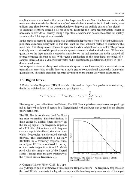
The FIR filter is not the one used for filtering
prior to sampling. This band-limiting is
done earlier by analog filters directly on
the analog signal. The frequency response
of a FIR filter determines which frequencies
are kept in the filtered signal and thus
which frequencies are discarded through
filtering. This characteristic is typically
illustrated by a frequency response curve
as in figure 12. The normalized frequency
on the x-axis ranges from 0 to 0.5. Multiplied
with the sample rate of the filtered
signal it ranges from the zero frequency to
the Nyquist critical frequency .
f c
Magnitude
A Quadrate Mirror Filter (QMF) is a specially
designed pair of distinctive Finite Impulse Response filters. The frequency responses of
the two FIR filters separate the high-frequency and the low-frequency components of the input
1.5
1
0.5
v i
m
∑
i = 0
– + i
FIR−Filter
0
0 0.05 0.1 0.15 0.2 0.25 0.3 0.35 0.4 0.45 0.5
Normalized Frequency
FIGURE 12. the frequency response curve of a Finite
Impulse Respond filter
w n