CAGD II – COURSE PROJECT
CAGD II – COURSE PROJECT
CAGD II – COURSE PROJECT

Create successful ePaper yourself
Turn your PDF publications into a flip-book with our unique Google optimized e-Paper software.
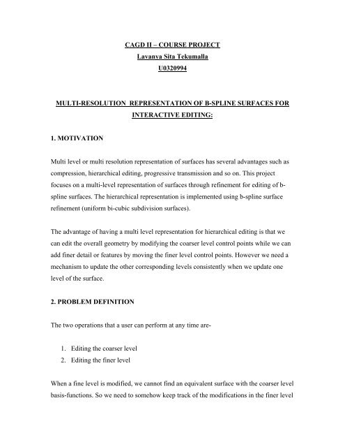
<strong>CAGD</strong> <strong>II</strong> <strong>–</strong> <strong>COURSE</strong> <strong>PROJECT</strong><br />
Lavanya Sita Tekumalla<br />
U0320994<br />
MULTI-RESOLUTION REPRESENTATION OF B-SPLINE SURFACES FOR<br />
1. MOTIVATION<br />
INTERACTIVE EDITING:<br />
Multi level or multi resolution representation of surfaces has several advantages such as<br />
compression, hierarchical editing, progressive transmission and so on. This project<br />
focuses on a multi-level representation of surfaces through refinement for editing of bspline<br />
surfaces. The hierarchical representation is implemented using b-spline surface<br />
refinement (uniform bi-cubic subdivision surfaces).<br />
The advantage of having a multi level representation for hierarchical editing is that we<br />
can edit the overall geometry by modifying the coarser level control points while we can<br />
add finer detail or features by moving the finer level control points. However we need a<br />
mechanism to update the other corresponding levels consistently when we update one<br />
level of the surface.<br />
2. PROBLEM DEFINITION<br />
The two operations that a user can perform at any time are-<br />
1. Editing the coarser level<br />
2. Editing the finer level<br />
When a fine level is modified, we cannot find an equivalent surface with the coarser level<br />
basis-functions. So we need to somehow keep track of the modifications in the finer level
separately. And when the coarser geometry is updated, make the appropriate changes to<br />
the finer geometry.<br />
Another idea that has been tried is, when we update the finer level, try and update the<br />
coarser geometry and get the closest possible approximation to the finer geometry in the<br />
least square sense (since we cannot get an exact representation using the basis functions<br />
of the coarser level)<br />
Also we need a means to specify motion of control point in 3D. This has been done by<br />
computing the partial derivatives and the normal of the surface at the node value<br />
corresponding to the control point.<br />
3.1 SPECIFYING CONTROL POINT POSITION BY DEFINING A LOCAL<br />
COORDINATE SYSTEM<br />
Specifying motion in 3D is a difficult problem. So instead when a user selects a control<br />
point and wants to move it, an orthonormal basis (u1,v1,n1) is displayed at that point with<br />
normal n1 pointing to the normal to the surface at that point, and u1 and v1 in the tangent<br />
plane at that point. This makes it intuitive and easy to specify motion.
Computing the Local basis system:<br />
Computing ∂suv ( , )/ ∂u:<br />
For every column j, the control points of the surface<br />
corresponding to the partial derivative with respect to u are computed as<br />
( Pi + 1, j−Pi, j)<br />
udeg<br />
(uk[i+udeg+1]-uk[i+1])<br />
Computing ∂suv<br />
( , ) / ∂v:<br />
For every row i, the control points of the surface corresponding<br />
to the partial derivative with respect to u are computed as<br />
( Pi, j + 1 − Pi, j)<br />
vdeg<br />
(vk[j+vdeg+1]-vk[j+1])<br />
Where udeg is the degree in the u direction, vdeg the degree in the v direction, uk the u<br />
knot vector and vk the v knot vector.<br />
The knot vector of the new spline surface (partial derivative) is similar to the original<br />
knot vector, it is uniform floating with two fewer elements compared to the original.<br />
When we want to move a particular control point, the node value in the parameter space<br />
corresponding to that control point is taken <strong>–</strong> say this is (u,v)<br />
The normal is computed as n= ∂suv ( , ) / ∂ ux<br />
∂suv ( , ) / ∂ v<br />
The local basis chosen is ∂suv ( , ) / ∂ u,<br />
∂suv ( , ) / ∂ ux<br />
n, n. The amount of motion in each<br />
of these directions is specified by the user using sliders in the GUI.
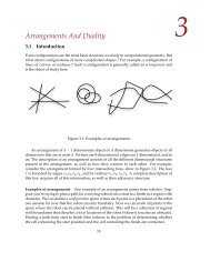
3.2 UNIFORM BI_CUBIC SUBDIVISION (CATMULL_CLARK SUBDIVISION)<br />
R i-2,j+2<br />
Pi/2-1, j/2+1<br />
R i-2,j+1<br />
R i-2,j<br />
Pi/2-1, j/2<br />
R i-2,j-1<br />
R i-2,j-2<br />
Pi/2-1, j/2-1<br />
R i-1,j+2<br />
R i-1,j+1<br />
R i-1,j<br />
R i-1,j-1<br />
R i-1,j-2<br />
R i,j+2<br />
Pi/2, j/2+1<br />
R i,j+1<br />
R i,j<br />
Pi/2, j/2<br />
R i,j-1<br />
R i,j-2<br />
Pi/2, j/2-1<br />
R i+1,j+2<br />
R i+1,j+1<br />
R i+1,j<br />
R i+1,j+1<br />
R i+1,j+2<br />
R i+2,j+2<br />
Pi/2+1, j/2+1<br />
R i+2,j+1<br />
R i+2,j<br />
Pi/2+1, j/2<br />
R i+2,j-1<br />
R i+2,j-2<br />
Pi/2+1, j/2-1<br />
This method proceeds by inserting a new knot between adjacent knots in the coarser<br />
surface and finding the corresponding new control points in terms of the old control<br />
points.<br />
The Subdivision Template<br />
For every control point Ri,j on the refined mesh, the Catmull-Clark subdivision template<br />
can be expressed as follows<br />
If i is odd and j is odd<br />
Ri,j = P(i/2 + ½, j/2 + ½) + P(i/2 + ½, j/2 - ½) + P(i/2 - ½, j/2 + ½) + P(i/2 - ½, j/2 - ½)<br />
If i is odd and j is even<br />
Ri,j = P(i/2 + ½, j/2 ) * 3/8+ P(i/2 + ½, j/2) *3/8<br />
+ P(i/2 - ½, j/2 + 1) *1/16 + P(i/2 - ½, j/2 + 1) * 1/16<br />
+ P(i/2 - ½, j/2 - 1) *1/16 + P(i/2 + ½, j/2 - 1) *1/16
If i is even and j is odd<br />
Ri,j = P(i/2 , j/2 <strong>–</strong> 1/2) * 3/8+ P(i/2 , j/2 + 1/2) *3/8<br />
+ P(i/2 - 1, j/2 + 1/2) *1/16 + P(i/2 + ½, j/2 + 1/2) * 1/16<br />
+ P(i/2 - 1, j/2 <strong>–</strong> 1/2) *1/16 + P(i/2 + 1, j/2 <strong>–</strong> 1/2) *1/16<br />
If i is even and j is even<br />
Ri,j = P(i/2 , j/2 ) * 9/16<br />
+ P(i/2 , j/2 + 1) * 3/32 + P(i/2 , j/2 <strong>–</strong> 1) * 3/32<br />
+ P(i/2 + 1, j/2 ) * 3/32 + P(i/2 -1, j/2 ) *3/32<br />
+ P(i/2 - 1, j/2 -1) *1/64 + P(i/2 - 1, j/2 +1) *1/64<br />
+ P(i/2 + 1, j/2 + 1) *1/64 + P(i/2 + 1, j/2 <strong>–</strong> 1) *1/64<br />
3.3 FINDING THE CLOSEST ESTIMATE OF THE CONTROL POINTS OF THE<br />
BASE MESH<br />
Let M be the number of rows in the control mesh and N the number of columns<br />
The above template can be expressed as follows.<br />
For every control point Ra,b of the refined mesh,<br />
R<br />
M−1 N−1<br />
a, b = ∑ ∑<br />
i= 0 j=<br />
0<br />
Pijwij (, ) (, )<br />
where w(i,j) is defined by the template mentioned above if Ra,b contributes towards Pi,j<br />
and 0 otherwise.<br />
In other words, for all Ri where Ri is a control point belonging to the refined mesh,<br />
MN −1<br />
Ri = Pj * wj<br />
∑<br />
j=<br />
0<br />
This is a linear system and can be expressed as<br />
W P = R<br />
Where P is a (MN x 1) matrix<br />
Where R is a ((2M-3 * 2N-3) x 1) matrix<br />
And W is a ((2M-3 * 2N-3) x MN) matrix
Given a refined mesh, the R matrix is known, and the W matrix is known from the<br />
subdivision template. We can try to solve this system of equations and try to obtain a<br />
base mesh corresponding to this refined mesh. However, the above linear system is over<br />
determined. Hence Singular value decomposition has been used to solve this linear<br />
system in order to get the closest base mesh in the least squares sense.<br />
4 IMPLEMENTATION<br />
At any point of time, there are two surfaces objects that the user can access, the base<br />
surface B and the refined Surface S. Also In the program, every refined surface object<br />
has associated with it a base surface object (Sb). This base surface is a data member of<br />
the refined surface.<br />
Let u be the unit vector in the direction of partial of the surface with respect to u<br />
direction at that point. Let v be the unit vector in the direction of partial of the surface<br />
with respect to v direction at that point and let n be the unit vector in the direction of<br />
cross product of u and v (perpendicular to the tangent plane)<br />
Modifying Base Surface B --> B’<br />
The control points of the surface B are just set to the new values corresponding to B’ as<br />
specified interactively by the user.<br />
However, this change needs to be reflected in the refined mesh S too. Since the refined<br />
surface S might have been updated in the meantime, the amount by which it has been<br />
updated is obtained as follows.<br />
Its base surface Sb is invoked and subdivided adequate number of times to obtained the<br />
refined mesh Ss (This would have been our refined mesh if S has not been updated at<br />
any point of time). Each control point of Ss and S are compared, and their difference is<br />
split into three components along the directions u, v and n at that point. These differences<br />
are stored in a matrix D
Now the new base mesh B’ is copied into Sb and S is obtained by refining Sb by the<br />
adequate levels. Now the control points of S are modified according to the matrix D. In<br />
other words, each control point of S is displaced along its u, v, and n directions<br />
according to the values stored in D. We thus get our new refined surface S.<br />
When Refined Surface is Updated S -> S’<br />
The control points of the surface S are just set to the new values corresponding to S’ as<br />
specified interactively by the user.<br />
There is a checkbox to specify the option of attempting to update the base mesh<br />
adequately. If this box is checked, the base mesh is changed so that it is as close to the<br />
refined mesh as possible. Now B and Sb are updated to this new base mesh.<br />
5 SOLVING AN OVER DETERMINED SET OF EQUATIONS<br />
Suppose we have a set of equations AX=B .<br />
The number of unknowns (dimension of X) is n and the number of equations is m. In our<br />
case, m>n.<br />
|AX-B| is called the residue .<br />
Since the system is over determined, the matrix A is singular and is not invertible. Under<br />
these circumstances, commonly, we try to find a solution that minimizes the least square<br />
norm |Ax-B| 2 . When we put the partial derivative of this expression with respect to x to<br />
0, we end up with the expression<br />
A t A x-A t B=0<br />
Or A t A x=A t B<br />
These are called the normal equations.<br />
And x= (A t A) -1 A t B<br />
The Expression A + = [(A t A) -1 A t ] is called the pseudo inverse of the Matrix A.<br />
A + is also called the Morse Penrose inverse <strong>–</strong> since A + satisfies A A + A = A
Finding the Pseudo inverse of Matrix<br />
Finding the inverse of a matrix by the usual method (Adj(A)/Det(A)) is an extremely<br />
tedious process and is hardly ever used.<br />
The following are some of the common techniques employed in order to solve our system<br />
Ax=B<br />
Cholesky Factorization<br />
Every positive definite matrix A can be factored uniquely into the product<br />
A=Transpose(L)*L where L is a lower triangular matrix. This is the Cholesky<br />
factorization.<br />
• Split A t A into L t L where L is a Lower triangular matrix.<br />
• Let W= Lx<br />
• Solve the lower triangular system L t W = A t B<br />
• Now solve the upper triangular system L x = W<br />
• The time complexity of this algorithm is of the order O(mn 2 + n 3 /3)<br />
QR Decomposition:<br />
QR factorization is a more modern way of solving the least squares problem. Given a<br />
matrix A, it can be decomposed into an upper triangular matrix R and an orthogonal<br />
Matrix Q (QQ t =I)<br />
• Decompose A as A= Q R<br />
• Q R x = B<br />
• R x = (Q t B)<br />
This is an upper triangular system and can be solved by back substitution. This method<br />
gives us technique for finding the least squares approximation to the solution<br />
Complexity (2mn 2 <strong>–</strong> 2/3 n 3 )
Singular Value Decomposition<br />
Every m x n matrix A with m>n can be decomposed into<br />
A = U D V t<br />
Where D is a diagonal matrix and U and V are orthogonal matrices.<br />
Our system of equations is A x = B<br />
• Obtain the singular value decomposition if A A = U D V t<br />
• U D V t x = B<br />
• x= (U D V t ) -1 B<br />
• x = (V D -1 U t ) B<br />
A + = (V D -1 U t ) [the pseudo inverse of A]<br />
Cost : 2 mn 2 + 11 n 3<br />
Comparison of methods:<br />
Condition number is the ratio of the largest singular value to the smallest singular value<br />
and when the condition number is too large, the matrix is ill-conditioned.<br />
Solving by Cholesky factorization is more efficient than SVD. However, for ill-<br />
conditioned matrices, the condition number of A t A is the square of condition number of<br />
A (The eigen decomposition of A t A is VD 2 V t if singular value decomposition of A is<br />
UDV t ) . Hence solving the normal equations directly might have numerical instability<br />
issues. Hence SVD or QR factorization methods are generally preferred.<br />
When the rank of A is equal to n, the least squares problem has a unique solution.<br />
However when rank(A) < min(m , n) -- in other words, A is rank-deficient - we seek the<br />
minimum norm least squares solution x which minimizes both and .<br />
And SVD provides such a solution. For matrices that are not rank deficient, QR is the<br />
preferred method as it is cheaper than SVD when m and n are almost equal.<br />
However, When m>>n, the two methods have almost the same time complexity. And<br />
SVD is the method used in this project
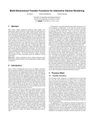
6. RESULTS<br />
1. Finding the refined mesh when the base mesh is updated<br />
The original base mesh The original refined mesh<br />
A control point in the refined mesh being<br />
moved<br />
New Base mesh after a control point in the base<br />
mesh has been moved<br />
New refined mesh after a control point in the<br />
refined mesh has been moved<br />
New refined mesh reflecting the change made to the<br />
base mesh and retaining its detail previously added.
2. Finding the closest base mesh given the refined mesh<br />
Original Base mesh Original Refined mesh<br />
Refined mesh being changed (A control point is<br />
being moved)<br />
New refined mesh New base mesh- updated going by the idea<br />
previously described
A closer view of the new refined mesh<br />
7. THE GUI<br />
`````<br />
A closer view of the new base mesh- updated<br />
going by the idea previously described
Exit: Exit the application<br />
New File: Read a new base mesh and get the appropriate refined mesh<br />
Write To File: Write the current mesh base/refined to file.<br />
Print Surface: Print the control mesh and knot vector of the current object to console<br />
Base: Show the base mesh<br />
Refined: Show the refined mesh<br />
Levels: Specify how many levels the refined mesh must be subdivided from the base<br />
mesh.<br />
Reset Transformations: Reset all the transformations done to the object so far (rotation,<br />
translation and scalling)<br />
U,V,N: Specify how much to move a control point along its u, uxn and n directions<br />
Fix movement: Fix the movement specified by the u, v and n sliders and update the<br />
surfaces<br />
Update Base: Update the base mesh when the refined mesh is modified<br />
Hide Curve/Surface: Do not show the surface when checked<br />
Hide other surface: Do not show the refined mesh when the current object is the base<br />
mesh, and vice versa<br />
Previous: When we modify the current object, when this box is checked, the object prior<br />
to the modification is shown in a different color.<br />
Hide Control Polygon: Hide the control polygon or the control mesh of the surface.<br />
The object under consideration can be rotated by moving the left mouse button, zoomed<br />
using the right mouse button and translated using the center mouse button. Any control<br />
point can be selected by clicking on it and it can be moved along u, v and n as specified<br />
using the sliders provided<br />
References:<br />
Elaine Cohen Richard F Riesenfeld Greshon Elber, “Geometric Modelling with Splines- An<br />
introduction”<br />
Numerical Recipes - http://www.library.cornell.edu/nr/cbookcpdf.html