to the I(1) - Feweb

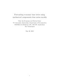
Introduction
Econometrics II – Chapter 7.5
Regression model with lags
One-equation cointegration
Marius Ooms
Tinbergen Institute Amsterdam
Section 7.5 considers bivariate dynamic processes with a
dynamic regression interpretation.
One variable is considered dependent and, in addition to
lagged values of the dependent variable, current and
lagged values of the other explanatory variable, that is
considered predetermined in the equation.
Such a relation is called an autoregressive distributed
lag (A(R)DL) relation. MA error terms can sometimes be
allowed for. We first assume joint stationarity of y and x for
estimation purposes: ”I(0)” world.
Chapter 7.5 – p. 1/30
Chapter 7.5 – p. 3/30
Contents
Introduction
Autoregressive Distributed Lag Model in I(0) world
Equilibrium Correction Model (ECM) in I(0) world
long run equilibrium
equilibrium correction
other economic dynamic regression models
(non)exogeneity, consequences
Cointegration: ADL/ECM in I(1) world
spurious regression
cointegration
Structural interpretation
Lagged dependent terms in A(R)DL models motivated by
economic theory (partial adjustment, adaptive
expectations, equilibrium correction), rather than just
modelling serial correlation: the ADL model is a structural
equation with interpretable parameters.
Interpretation and estimation parameters depends on
exogeneity assumptions on x.
Example §7.5: yt: US inflation. xt: US tbill rate. See below.
Chapter 7.5 – p. 2/30
Chapter 7.5 – p. 4/30

AR distributed lag model (ADL(p,r))
We study the ADL(1, 1) model
yt = α + φyt−1 + β0xt + β1xt−1 + εt,
where |φ| < 1: stability condition in this context. The error
term, εt, is White Noise. xt is considered predetermined in
the equation or, in more general terms: (weakly)
exogenous with respect to the estimation of the
parameters α, φ, β0 and β1. This requires that xt is
uncorrelated with εt,εt+1,....
The model can be re-formulated in DL(∞) form to show
the response of yt,yt+1,... to one-time changes in xt:
dynamic impact (”impulse response”)
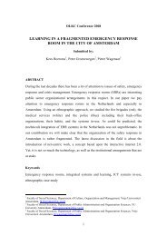
ARDL example US inflation, Interest rates
US Core inflation (SA), 3-month T-bill, 59.1-99.12
24
20
16
12
8
4
0
-4
-8
60 65 70 75 80 85 90 95
USCOREINFSA TBAA3M
Chapter 7.5 – p. 5/30
Chapter 7.5 – p. 7/30
Dynamic impact, ARDL(0,∞) form of ARDL(1,1)
(1 − φL)yt = α + (β0 + β1L)xt + εt,
φ(L)yt = α + β(L)xt + εt,
yt = αφ −1 (1) + φ −1 (L)β(L)xt + φ −1 (L)εt.
∂yt
∂xt
∂yt+1
∂xt
∂yt+j
= β0,
= β1 + φβ0,
.
∂xt
= φ j−1 (β1 + φβ0), for j > 0.
Note that the influence on yt+j disappears as j → ∞.
ARDL(6,4) estimation example ’reduced form’
Modelling UScoreinfSA by OLS
The estimation sample is: 62 (1) to 99 (12)
Coefficient Std.Error t-value t-prob
UScoreinfSA_1 0.233366 0.04750 4.91 0.000
...
UScoreinfSA_6 0.102451 0.04612 2.22 0.027
Constant 0.239006 0.3136 0.762 0.446
tbaa3m 0.867091 0.2383 3.64 0.000
tbaa3m_1 -0.646922 0.3798 -1.70 0.089
...
tbaa3m_4 -0.340460 0.2405 -1.42 0.158
sigma 2.54947 RSS 2885.89892
Rˆ2 0.542968 F(11,444) = 47.95 [0.000]**
log-likelihood -1067.72 DW 2.04
no. of observations 456 no. of parameters 12
mean(UScoreinfSA) 4.54782 var(UScoreinfSA) 13.8475
Chapter 7.5 – p. 6/30
Chapter 7.5 – p. 8/30

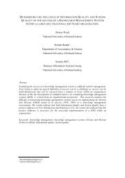
ARDL dynamic impact of x, example
Dynamic impact interest rate on inflation (scaled, sum=1)
2
1
0
−1
2.5
2.0
1.5
1.0
tbaa3m
Impact tbaa3m (normalized) on UScoreinfSA
0 5 10 15 20 25 30
tbaa3m(cum)
Cumulative impact tbaa3m (normalized) on UScoreinfSA
0 5 10 15 20 25 30 35 40
Long-run elasticity
When y,x is in logs, then
λ = β(1)
φ(1) =
∞
j=0
∂yt+j
∂xt
can be interpreted as a “long-run elasticity”.
Chapter 7.5 – p. 9/30
Chapter 7.5 – p. 11/30
Long run “equilibrium relationships” from ADL eq.
Thought experiment: keep xt = ¯x constant, put all εt = 0
and compute the value for yt after convergence (assuming
this is the only dynamic relationship between xt and yt),
that is ¯y.
The “equilibrium” is
or, in general,
¯y = δ + φ¯y + β0¯x + β1¯x,
¯y = α β(1)
+
φ(1) φ(1) ¯x.
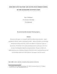
Long run relation Inflation Interest Rate?
US interest rate vs. inflation 62-99(Fisher equation)
USCOREINFSA
24
20
16
12
8
4
0
-4
-8
2 4 6 8 10 12 14 16 18
TBAA3M
Chapter 7.5 – p. 10/30
Chapter 7.5 – p. 12/30

Long run equation implied by ARDL
By simple calculations one can derive a long run relation
between x and y from the ARDL and test its significance:
Solved static long run equation for UScoreinfSA
Coefficient Std.Error t-value t-prob
Constant 1.07147 1.445 0.742 0.459
tbaa3m 0.558555 0.2175 2.57 0.011
ECM = UScoreinfSA - 1.07147 - 0.558555*tbaa3m; (Equilibrium correction
mechanism)
Inverse Roots of UScoreinfSA lag polynomial (is AR part stable?):
real imag modulus
0.92014 0.00000 0.92014
0.32600 0.61182 0.69326
...
-0.34068 -0.48614 0.59363
How to derive the Equilibrium correction term? See next!
Example: ECM unrestricted: eq. (2)
Exercise (1): Compute long run semi- elasticity λ from OLS
output:
Dependent Variable: DUSCOREINFSA
Method: Least Squares
Sample: 1962:01 1999:12
Included observations: 456
Variable Coefficient Std. Error t-Statistic Prob.
C 0.239006 0.313641 0.762036 0.4464
DUSCOREINFSA(-1) -0.543571 0.063107 -8.613422 0.0000
DUSCOREINFSA(-2) -0.319701 0.064293 -4.972542 0.0000
DUSCOREINFSA(-3) -0.297513 0.061498 -4.837784 0.0000
DUSCOREINFSA(-4) -0.206045 0.058424 -3.526735 0.0005
DUSCOREINFSA(-5) -0.102451 0.046116 -2.221614 0.0268
DTBAA3M 0.867091 0.238304 3.638592 0.0003
DTBAA3M(-1) 0.095577 0.247830 0.385655 0.6999
DTBAA3M(-2) 1.090760 0.243602 4.477637 0.0000
DTBAA3M(-3) 0.340460 0.240463 1.415852 0.1575
USCOREINFSA(-1) -0.223063 0.053931 -4.136090 0.0000
TBAA3M(-1) 0.124593 0.063355 1.966567 0.0499
R-squared 0.393532 Mean dependent var 0.003614
Adjusted R-squared 0.378507 S.D. dependent var 3.233931
S.E. of regression 2.549465 Akaike info criterion 4.735608
Sum squared resid 2885.899 Schwarz criterion 4.844094
Log likelihood -1067.719 F-statistic 26.19159
Durbin-Watson stat 2.040891 Prob(F-statistic) 0.000000
Chapter 7.5 – p. 13/30
Chapter 7.5 – p. 15/30
Equilibrium (Error) Correction Model (E(q)CM)
The ECM explains the change in y using one lagged level
of y and x and one or more lagged differences of y and
x. The ECM representation of the ADL model is easier to
interpret and often easier to estimate. In the univariate
case, β(L) = 0, it reduces to an (A)D-F regression.
yt = α + φyt−1 + β0xt + β1xt−1 + εt, (1)
∆yt = α − (1 − φ)yt−1 + β0∆xt + (β0 + β1)xt−1 + εt, (2)
= β0∆xt − (1 − φ)[yt−1 − δ − λxt−1] + εt, (3)
δ =
α
(1 − φ) , λ = (β0 + β1)
(1 − φ) .
δ and λ are ‘the ‘equilibrium” coefficients.
Decomposition ECM model
The ECM specification (3) decomposes a change in y into
two components,
1. from change in x: ∆xt: direct short run effect
2. from lagged equilibrium error: zt−1 where
zt = yt − δ − λxt
When yt is higher than equilibrium value (positive z), y will
adjust downwards in order to get back to equilibrium:
Equilibrium (error) correction.
Remember: §7.5 assumes there is no feedback (Granger
non-causality) from y to x!
Chapter 7.5 – p. 14/30
Chapter 7.5 – p. 16/30

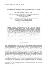
Example: ECM term time series plot
20
15
10
5
0
-5
-10
-15
ECM term = UScoreinfSA - 1.07 - 0.56*tbaa3m
1965 1970 1975 1980 1985 1990 1995
ECMTERM
Chapter 7.5 – p. 17/30
Partial Scatterplot ECM effect, (c.f. §3.2.5 Case 3)
DUSCOREINFSAPARTIAL vs. ECMTERMLAGGEDPARTIAL
DUSCOREINFSAPARTIAL
15
10
5
0
-5
-10
-6 -4 -2 0 2 4 6 8 10
ECMTERMLAGGEDPARTIAL
Chapter 7.5 – p. 19/30
Example: ECM estimation eq. (3) with known λ
Exercise (2): Compute ”adjustment coefficient” (− φ(1)
from OLS output.
Dependent Variable: DUSCOREINFSA
Method: Least Squares
Sample(adjusted): 1962:02 1999:12
Included observations: 455 after adjusting endpoints
Variable Coefficient Std. Error t-Statistic Prob.
C 0.001846 0.119532 0.015444 0.9877
DUSCOREINFSA(-1) -0.543513 0.061869 -8.784847 0.0000
DUSCOREINFSA(-2) -0.319760 0.063442 -5.040161 0.0000
DUSCOREINFSA(-3) -0.298213 0.060994 -4.889204 0.0000
DUSCOREINFSA(-4) -0.205761 0.058014 -3.546746 0.0004
DUSCOREINFSA(-5) -0.104175 0.046282 -2.250878 0.0249
DTBAA3M 0.868916 0.236007 3.681734 0.0003
DTBAA3M(-1) 0.093375 0.245796 0.379888 0.7042
DTBAA3M(-2) 1.093816 0.242643 4.507912 0.0000
DTBAA3M(-3) 0.339643 0.239119 1.420392 0.1562
ECMTERM(-1) -0.223273 0.052104 -4.285112 0.0000
R-squared 0.393677 Mean dependent var 0.003294
Adjusted R-squared 0.380021 S.D. dependent var 3.237484
S.E. of regression 2.549155 Akaike info criterion 4.733280
Sum squared resid 2885.197 Schwarz criterion 4.832891
Log likelihood -1065.821 F-statistic 28.82824
Durbin-Watson stat 2.039039 Prob(F-statistic) 0.000000
Direct estimation ECM λ and s.e. in Eviews
Chapter 7.5 – p. 18/30
(Advanced) Exercise (3): Explain why the coefficient of rt
is estimated using 2SLS and why it is a consistent estimate
of λ. Hint: Apply the decomposition α0 + α1L = α(1) − α1∆
to φ(L) and β(L).
Dependent Variable: USCOREINFSA
Method: Two-Stage Least Squares
Date: 02/10/03 Time: 10:51
Sample: 1962:01 1999:12
Included observations: 456
Instrument list: C TBAA3M DTBAA3M(0 TO -3) DUSCOREINFSA(-1
TO -5) USCOREINFSA(-1)
Variable Coefficient Std. Error t-Statistic Prob.
C 1.071473 1.444886 0.741562 0.4587
TBAA3M 0.558555 0.217458 2.568569 0.0105
DUSCOREINFSA -3.483041 1.083884 -3.213482 0.0014
DUSCOREINFSA(-1) -2.436850 0.808796 -3.012937 0.0027
DUSCOREINFSA(-2) -1.433233 0.555871 -2.578358 0.0102
DUSCOREINFSA(-3) -1.333765 0.507371 -2.628777 0.0089
DUSCOREINFSA(-4) -0.923709 0.398263 -2.319342 0.0208
DUSCOREINFSA(-5) -0.459293 0.257246 -1.785425 0.0749
DTBAA3M 3.328652 1.381126 2.410101 0.0164
DTBAA3M(-1) 0.428475 1.124256 0.381118 0.7033
DTBAA3M(-2) 4.889923 1.678523 2.913231 0.0038
DTBAA3M(-3) 1.526295 1.140696 1.338038 0.1816
R-squared -8.185267 Mean dependent var 4.547815
Adjusted R-squared -8.412830 S.D. dependent var 3.725304
S.E. of regression 11.42936 Sum squared resid 57999.81
F-statistic 2.386014 Durbin-Watson stat 2.040891
Prob(F-statistic) 0.007054
Chapter 7.5 – p. 20/30

Partial Adjustment interpretation ADL(1,0)
NB: in following two examples: λ is an adjustment
parameter, not equilibrium parameter. δ is equilibrium
parameter, not a constant term.
Partial adjustment
The economic structural model:
with ADL model:
yt = yt−1 + λ(y ∗ t − yt−1) + εt
y ∗ t = γ + δxt
yt = λγ + (1 − λ)yt−1 + λδxt + εt : ADL(1, 0).
Exercise (4): Derive this ADL model.
(Weak) exogeneity
Chapter 7.5 – p. 21/30
In the context of ECM models one often extends the old
concept of predeterminedness (“independence” of
regressor variable and present and future structural
equation errors) to the concept of weak exogeneity. (Short:
exogeneity in §4.1.3: plim 1
n X′ ε) = 0).
A variable xt is said to be weakly exogenous for estimating
a parameter of interest λ, if inference on λ conditional on xt
involves no loss of information. In practice joint modelling
of yt and xt does not improve inference on λ if xt is weakly
exogenous.
Strict exogeneity: “Independence” of regressors and
structural equation errors at all leads and lags, does not
apply to ECM.
Chapter 7.5 – p. 23/30
Adaptive expectations ARDL(1,0)-MA(1)
Adaptive Expectations
The economic structural model, where the true explanatory
variable (i.c. expected x) x ∗ t+1 is unobserved.
yt = γ + δx ∗ t+1 + εt
x ∗ t+1 = x ∗ t + λ(xt − x ∗ t)
The corresponding ARDL(1,0) form has MA(1) errors
yt = λγ + (1 − λ)yt−1 + λδxt + εt − (1 − λ)εt−1,
which can also be written in ARDL(0,∞) form:
yt = γ + (1 − (1 − λ)L)) −1 λδxt + εt.
Exercise (5): derive this ARDL(0,∞) form.
Strong exogeneity, Granger non-causality
The ADL model can be used as part of a forecasting
procedure for yt. If we want efficient inference on future yt
without making a joint dynamic model for yt and xt we
need a strong exogeneity assumption.
Strong Exogeneity of xt for (forecasting) equation yt
combines two requirements:
1. (Weak) exogeneity of xt for estimating all the
parameters of the equation for yt
2. Granger non-causality of yt for xt, §7.6.2
In linear forecasting of xt using lags of xt, additional
lags of yt do not decrease forecast MSE: Partial
correlations of xt with yt−1,yt−2,... are zero.
Regression F -test for Granger-noncausality in
auxiliary equation for xt.
Chapter 7.5 – p. 22/30
Chapter 7.5 – p. 24/30

Extending ARDL from the I(0) to the I(1) world
The ARDL model can also be used for nonstationary
series, but then one has to be careful with statistical
inference. Standard distribution theory does not apply. In
the I(1) world the notion of long run equilibrium
corresponds to cointegration and the existence of a
common trend.
Cointegration does not require strong exogeneity of x for
the estimation of the parameters in the ARDL equation(s).
It does require I(1)-ness of both x and y.
Spurious regression, non-cointegration
Regress I(1) process yt on independent I(1) process xt.
This means the residual process is also I(1)!
OLS based inference (§2.3): Overrejection of H0 of
independence because of extremely strong positive serial
correlation in the error term.
GMM based inference (§5.5.3) (automatic “Newey-West
correction” for serial correlation in error term) does not
work for I(1) either. The moments of GMM do not exist!
Correction for determistic trend does not work either. The
’omitted trend variable’ is not observed!
Chapter 7.5 – p. 25/30
Chapter 7.5 – p. 27/30
Cointegration and Spurious Regression
Definition cointegration: yt, xt ∼ CI(1, 1):
yt ∼ I(1), xt ∼ I(1), linear combination (yt − λxt) ∼ I(0).
yt − λxt integrated of order 1-1=0. Cointegration concerns
only the stochastic part of series, i.e. not the deterministic
part.
Spurious regression:
yt ∼ I(1), xt ∼ I(1), yt and xt independent, regress yt on
constant and xt (so that residuals of spurious regression
are also I(1)).
Spurious regression problem:
Apply assumption of I(0) (or even WN) to I(1) variables in
assessing statistical significance of correlations and
regression coefficients. Result: incorrect rejection of H0 :
“no linear relationship”.
Cointegration in the ADL model
Consider the ARDL model with xt ∼ I(1):
yt = α + φyt−1 + β0xt + β1xt−1 + εt
xt = xt−1 + ηt
Chapter 7.5 – p. 26/30
with εt, ηt independent WN, |φ| < 1, β0 + β1 = 0, so
xt ∼ I(1) and yt = (1 − φL) −1 [α + β0xt + β1xt−1 + εt] ∼ I(1).
There is no long run equilibrium value for x.
∆yt is a stationary, invertible ARMA(1,1) process and
therefore I(0). This means yt is I(1).
yt fluctuates around [α0 + (β0 + β1)xt]/(1 − φ).
One can show that yt and xt are cointegrated with one
common trend: (1 − L) −1 ηt.
Chapter 7.5 – p. 28/30

ARDL in ECM form in I(1) world
The error/equilibrium correction form is:
∆yt = β0∆xt − (1 − φ)zt−1 + εt,
where deviation from equilibrium zt is defined as
zt = yt −
α
(1 − φ) − (β0 + β1)
(1 − φ) xt.
Advanced Exercise (6): Prove zt is I(0), therefore xt and yt
are CI(1,1). Hint: Apply the ”unit root” decompositions
α0 + α1L = α(1) − α1∆ and/or α0 + α1L = α0∆ + α(1)L to
φ(L) and/or β(L). Note connection with Advanced Exercise
(3)
Chapter 7.5 – p. 29/30
Warning: Coefficient tests in ECM in I(1) world
OLS/GMM inference on coefficient tests in ECM with
possible I(1) regressors is not standard, not even without
serial correlation in the residuals. Some t− tests are
asymptotically normal. Some are not!
Standard I(0) inference: t-tests with standard normal tables.
Standard t-test examples, test for:
- φ = 0 (coeff of yt−1 in (2)): test immediate full adjustment of y to
disequilibrium.
- β0 = 0 (coeff of ∆xt in (2)): zero direct impact x on y.
Nonstandard t-test examples, test for
- (1 − φ) = 0 (coeff of yt−1 if no ECM): cf. Augmented DF,
- β0 + β1 = 0 (coeff for xt−1 in (2) if no ECM): a test for
non-cointegration. Warning: Coefficient tests involving I(1)
regressors under H0 can have nonstandard limiting distributions.
Chapter 7.5 – p. 30/30