Density dependent liquid Nitromethane decomposition: MD ...
Density dependent liquid Nitromethane decomposition: MD ...
Density dependent liquid Nitromethane decomposition: MD ...

Create successful ePaper yourself
Turn your PDF publications into a flip-book with our unique Google optimized e-Paper software.
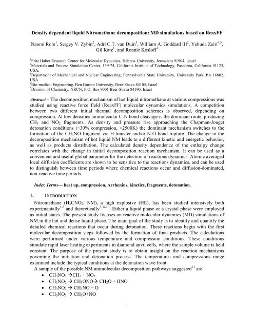
<strong>Density</strong> <strong>dependent</strong> <strong>liquid</strong> <strong>Nitromethane</strong> <strong>decomposition</strong>: <strong>MD</strong> simulations based on ReaxFF<br />
Naomi Rom 1 , Sergey V. Zybin 2 , Adri C.T. van Duin 3 , William A. Goddard III 2 , Yehuda Zeiri 4,5 ,<br />
Gil Katz 1 , and Ronnie Kosloff 1<br />
1<br />
Fritz Haber Research Center for Molecular Dynamics, Hebrew University, Jerusalem 91904, Israel<br />
2<br />
Materials and Process Simulation Center, 139-74, California Institute of Technology, Pasadena, California 91125,<br />
USA,<br />
3<br />
Department of Mechanical and Nuclear Engineering, Pennsylvania State University, University Park, PA 16802,<br />
USA<br />
4<br />
Bio-medical Engineering, Ben Gurion University, Beer-Sheva 84105, Israel<br />
5<br />
Division of Chemistry, NRCN, P.O. Box 9001 Beer-Sheva 84190, Israel<br />
Abstract – The <strong>decomposition</strong> mechanism of hot <strong>liquid</strong> nitromethane at various compressions was<br />
studied using reactive force field (ReaxFF) molecular dynamics simulations. A competition<br />
between two different initial thermal <strong>decomposition</strong> schemes is observed, depending on<br />
compression. At low densities unimolecular C-N bond cleavage is the dominant route, producing<br />
CH3 and NO2 fragments. As density and pressure rise approaching the Chapman-Jouget<br />
detonation conditions (~30% compression, >2500K) the dominant mechanism switches to the<br />
formation of the CH3NO fragment via H-transfer and/or N-O bond rupture. The change in the<br />
<strong>decomposition</strong> mechanism of hot <strong>liquid</strong> NM leads to a different kinetic and energetic behavior,<br />
as well as products distribution. The calculated density dependence of the enthalpy change<br />
correlates with the change in initial <strong>decomposition</strong> reaction mechanism. It can be used as a<br />
convenient and useful global parameter for the detection of reactions dynamics. Atomic averaged<br />
local diffusion coefficients are shown to be sensitive to the reactions dynamics, and can be used<br />
to distinguish between time periods where chemical reactions occur and diffusion-dominated,<br />
non-reactive time periods.<br />
Index Terms— heat up, compression, Arrhenius, kinetics, fragments, detonation.<br />
1. INTRODUCTION<br />
<strong>Nitromethane</strong> (H3CNO2, NM), a high explosive (HE), has been studied intensively both<br />
experimentally 1- 5 and theoretically 3, 6- 10 . Either a <strong>liquid</strong> phase or a crystal phase were employed<br />
as initial states. The present study focuses on reactive molecular dynamics (<strong>MD</strong>) simulations of<br />
NM in the hot and dense <strong>liquid</strong> phase. The main goal of the study is to identify and quantify the<br />
detailed chemical reactions that occur during detonation. These reactions begin with the first<br />
molecular <strong>decomposition</strong> steps followed by the formation of final products. The calculations<br />
were performed under various temperature and compression conditions. These conditions<br />
simulate rapid laser heating experiments in diamond anvil cells, where the sample volume is held<br />
constant. The purpose of the present study is to obtain insight on the reaction mechanisms<br />
governing the initiation and detonation process. The temperatures and compressions range<br />
examined include the typical conditions at the detonation wave front.<br />
A sample of the possible NM unimolecular <strong>decomposition</strong> pathways suggested 11 are:<br />
• CH3NO2 CH3 + NO2<br />
• CH3NO2 CH3ONO CH2O + HNO<br />
• CH3NO2 CH3NO + O<br />
• CH3NO2 CH3O+NO<br />
1
• CH3NO ↔ CH2NOH<br />
• CH3NO2CH2NOOH<br />
In a previous study 8 , the <strong>decomposition</strong> of solid NM was calculated using <strong>MD</strong> simulations<br />
with on-the-fly calculations of molecular forces with density functional theory. In these<br />
simulations, dense solid NM (1.97 g/cm 3 and 2.2 g/cm 3 ) was rapidly heated to 3000K and<br />
4000K. The first step revealed in the thermal <strong>decomposition</strong> was inter-molecular proton transfer<br />
forming [H3CNO2H] + and aci ion [H2CNO2] - . The second step observed was intra-molecular<br />
proton transfer forming aci acid [H2CNO2H]. Then, additional fragments were formed, such as:<br />
CH2NO + , OH - and H2O. These reaction products were related to condensed phase reactions,<br />
whereas C-N bond break, being the weakest in the molecule (D0=60.1 kcal/mol in the gas phase),<br />
prevails in gas phase or dilute fluid <strong>decomposition</strong>.<br />
The hypothesis that hydrogen abduction is the rate determining step at a pressure of 10 kbar<br />
and at a temperature of 273 o C, is supported by the measured time to detonation with deuterated<br />
NM which was found to be 10 times longer than with protonated NM 1 . However, interpolation to<br />
higher temperatures suggests that above 330 o C the time to denotation of NM is shorter than that<br />
of deuterated NM. Thus, possibly H-transfer is more important at similar compressions and<br />
lower temperatures (
section 5.<br />
2. COMPUTATIONAL APPROACH<br />
The parallel version of the ReaxFF-<strong>MD</strong> code 12, 13 , GRASP (General Reactive Atomistic<br />
Simulation Package) was used to study the behavior of <strong>liquid</strong> NM under various conditions.<br />
ReaxFF-<strong>MD</strong> was used in various applications, such as surface catalysis 14 and combustion<br />
chemistry 15 . In addition, it was used to study the initial chemical reactions that occur during<br />
thermal or shock induced <strong>decomposition</strong> of HE materials (e.g., NM 9 , RDX 16, 17 and TATP 18 ), and<br />
recently in the calculation of directional anisotropy in PETN single crystal resulting from<br />
combined shear and compressive loading 19 . Note that ReaxFF potentials were trained for ground<br />
state processes only, thus fragments obtained in these simulations are radicals or stable<br />
molecules (not ionic species). ReaxFF parameters were fitted to results of multiple ab initio<br />
quantum mechanical (QM) calculations. ReaxFF-<strong>MD</strong> simulations were shown to reproduce the<br />
QM results with high accuracy. Some examples 20 are: Bonds dissociation (gas phase reactions<br />
path), compression curves, geometry distortions (angles and torsion), charges, IR-spectra,<br />
condensed phase structures, gas phase reactions, and equations of state of molecules and crystals<br />
with H, C, N and O atoms.<br />
Below we describe the procedure employed to prepare the <strong>liquid</strong> samples at various<br />
compressions followed by the conditions used in the heat up simulations.<br />
2.1 Sample preparation<br />
Preparation of <strong>liquid</strong> NM starts with a solid slab in which the NM molecules are arranged<br />
according to their crystal structure. The molecular slab (supercell) is obtained by multiplying<br />
solid NM unit cell (orthorhombic cell, FIG. 1a, with a, b, c = 5.228, 6.293, 8.664 Å) by an<br />
integer along the different directions. Here: 5x4x3 expansion along x, y, and z directions was<br />
employed. Hence, the total number of molecules in the simulation was 240 (1680 atoms). Energy<br />
minimization is carried out to obtain optimized equilibrium geometry of the expanded crystal<br />
(FIG. 1b).<br />
(a)<br />
(b) (c)<br />
2.1.1 Liquid creation (ambient conditions).<br />
FIG. 1: NM Crystal. (a) unitcell (b) 5x4x3 energy minimized supercell and (c) <strong>liquid</strong> NM supercell at<br />
ambient conditions.<br />
In order to obtain a <strong>liquid</strong> structure at ambient conditions the following procedure was applied to<br />
the relaxed crystal supercell:<br />
• The cell volume was increased by 50%, then its energy minimized resulting in an<br />
optimized geometry (0.25ps).<br />
3
• The obtained supercell was heated to 400K (10ps), well above the NM melting point<br />
(244K).<br />
• The hot cell was heavily compressed (NPT simulation at 1 GPa and 400K, 30 ps).<br />
• Cooling and decompression was applied (NPT at 1atm and 300K, 30ps). Calculated mass<br />
density of the liquefied sample at the end of the simulation was 1.111gr/cm 3 (a, b, c =<br />
28.327, 27.386, 28.222 Å). It differs only by ~2% from the measured density 1.137<br />
gr/cm 3 .<br />
• The <strong>liquid</strong> cell was thermalized (NVT, T=300K, 2 ps), and pressure oscillations reduced<br />
to ±0.5GPa.<br />
• Finally the system state was relaxed (NVE simulation, 1ps). A typical <strong>liquid</strong> supercell is<br />
shown in FIG. 1c.<br />
The time step in all the calculations described above was 0.25 fs. In the simulations, a simple<br />
rescaling thermostat was used, with temperature correction proportional to half the difference<br />
between the target and current temperature.<br />
Radial distribution functions for the solid and <strong>liquid</strong> simulation cells are presented in FIG. 2.<br />
Here, r is the distance between two NM molecules. As expected, typical structured behavior and<br />
smooth modulations are obtained for the solid and <strong>liquid</strong> cells, respectively. Results are shown<br />
for r ≤ d/2, where d is the smallest cell vector.<br />
g(r)<br />
0.18<br />
0.16<br />
0.14<br />
0.12<br />
0.1<br />
0.08<br />
0.06<br />
0.04<br />
0.02<br />
NM Solid (1atm, 200K)<br />
0<br />
0 2 4 6 8 10 12 14<br />
r (A)<br />
FIG. 2: Radial distribution function for NM molecules in the solid (left) and <strong>liquid</strong> (right) phases. Distance<br />
units are Å.<br />
2.2 Liquid compression (T=300K, P=1atm)<br />
In order to obtain <strong>liquid</strong> in various compressions we began with the <strong>liquid</strong> sample prepared by<br />
the process described above and volumetrically compressed it by the desired amount. Then, it<br />
was energy-minimized for 0.5-1ps, depending on the magnitude of the compression, until<br />
equilibrium atomic positions were obtained. Finally, each sample was thermalized using NVT<br />
simulation at 300K (2ps), using a velocity rescaling thermostat. It is important to note that none<br />
of the NM molecules decomposed during these stages.<br />
2.3 Heat up simulations<br />
Heat up simulations of <strong>liquid</strong> NM were made in two stages: Initially, the sample at a fixed<br />
density was heated rapidly (within 100 fs, using time step 0.25 fs) from room temperature to the<br />
desired final temperature (Tf). Then, NVT simulations were carried out at Tf until the final<br />
products approached constant amounts. The rapid heating is carried out on a time scale similar to<br />
4<br />
g(r)<br />
0.12<br />
0.1<br />
0.08<br />
0.06<br />
0.04<br />
0.02<br />
NN Liquid (1 atm, 300K)<br />
0<br />
0 2 4 6 8 10 12 14<br />
r(A)
that of a detonation wave passing through the simulation cell (~500 fs). The time step used in<br />
NVT simulations was 0.1 fs, and the simulations progressed for 60-80 ps.<br />
Thermal rate constants were calculated at three regimes within the simulations:<br />
- Initial <strong>decomposition</strong> reaction/s (endothermic).<br />
- Intermediate reactions and products.<br />
- Stable products formation with the main products: H2O, CO2, N2, H2, CO and OH.<br />
The following section describes the methods employed for the chemical kinetics analysis.<br />
2.3.1 Chemical reactions and fragments analysis<br />
Fragments analysis was done with “BondFrag”, a code developed in Goddard’s group at Caltech.<br />
For each pair of atoms in the simulation cell a “bond order” is calculated. Then, according to<br />
cutoff values predefined for each pair (given in section 5), the code determines whether a<br />
chemical bond exists or not, thus fragments or molecules are being formed.<br />
According to the reaction regimes mentioned above, fragments were examined in three stages:<br />
Creation of primary fragments, representing a reaction bottleneck at the very beginning of <strong>liquid</strong><br />
NM <strong>decomposition</strong>; intermediate fragments formation, where many reactions occur<br />
simultaneously leading to multiple fragments (unstable and stable); and final products<br />
stabilization when thermodynamic equilibrium is reached. The main chemical reactions<br />
occurring in the initial stages of NM <strong>decomposition</strong> are listed below.<br />
2.3.2 Rate constants analysis<br />
Thermal rate constants were calculated as a function of density and temperature in the three<br />
different reaction stages. The average potential energy, PE, of the system was monitored during<br />
the simulation. It was found that PE exhibits a maximum close to the initial stages of the<br />
simulation. Fragments analysis (see section 3.4) reveals the nature of the peak: It roughly<br />
separates between the initial, endothermic <strong>decomposition</strong> of NM and the intermediate, multiple<br />
reactions stage. The time when the potential energy reaches a maximum, tmax, was determined for<br />
each simulation. This was accomplished by fitting a smooth function (sum of decreasing and<br />
increasing exponential functions) to the evolution of PE during the simulation and finding its<br />
maximum. In cases where the PE maximum was too close to the simulation initiation (namely, at<br />
high temperatures), a local polynomial fit was applied in the vicinity of the PE maximum to get<br />
tmax, which was then used to distinguish between NM initial <strong>decomposition</strong> and the intermediate<br />
reactions stage.<br />
For each simulation, rate constants in the three stages are deduced as follows:<br />
• Initial <strong>decomposition</strong> stage rate constant, ρ, : The hot <strong>liquid</strong> NM molecules decay<br />
was fitted with a first order decay expression, N(t), from the beginning of the<br />
<strong>decomposition</strong>, at t0, until tmax:<br />
1. · exp <br />
Note that in previous works 7, 16 this fit was made along the full NM decay, including the<br />
zone where intermediate reactions take place and hence influence the rate constant,<br />
introducing inaccuracy into the single exponential function fit.<br />
• Intermediate <strong>decomposition</strong> stage, ρ, : Bypassing the complexity of chemical<br />
reactions at this stage, an effective first order rate constant is obtained by fitting a<br />
decaying exponential function to the decaying part of PE curve, U(t), starting from tmax:<br />
2. ∞ ∆ · exp <br />
5
U∞ is the asymptotic value of potential energy (products PE) and ΔUexo=U(tmax)-U∞. The<br />
latter is the exothermicity, or the heat release, in NM <strong>decomposition</strong> reaction. This type<br />
of fitting was also used in the thermal <strong>decomposition</strong> study of RDX 16 , TATB and HMX 20 .<br />
NM <strong>decomposition</strong> enthalpy change, ΔH, can be estimated from:<br />
3. ∆ ∆ ∞ <br />
As will be seen in section 3.6, ΔH seems to be correlated with the initial <strong>decomposition</strong><br />
mechanism of NM (which is pressure <strong>dependent</strong>). If so, it can serve as a simple yet<br />
sensitive tool in identifying mechanism changes under various conditions.<br />
• Final products evolution stage, k3: Effective rate constants (due to the variety of reactions<br />
leading to their formation) for final products creation can be calculated by fitting the<br />
following function to each product’s time evolution, C(t):<br />
4. ∞ · 1 <br />
ti is the product’s time of formation. Note that this fitting needs to be made until each<br />
product reaches stable amount, otherwise the fitted parameters will depend on the<br />
simulation length. C∞ is the estimated asymptotic amount of the products, and can be<br />
compared to measurements 22 and results of thermochemical computations 22 (see section<br />
3.5).<br />
Following the evaluation of the temperature and density <strong>dependent</strong> rate constants in the initial<br />
and intermediate <strong>decomposition</strong> stages of <strong>liquid</strong> NM, a fit to the Arrhenius equation is made to<br />
obtain activation energies and pre-exponential factors as a function of density for these stages.<br />
Kinetic analysis results are presented in the following section.<br />
2.3.3 Diffusion coefficient and mean square displacement of the atoms<br />
The mobility of atoms during the simulation is influenced by the pressure and temperature, as<br />
well as by their participation in chemical reactions. Diffusion coefficient, D, can be estimated<br />
using Einstein’s expression:<br />
<br />
5. ∑ 0 <br />
<br />
<br />
rj(t) is the coordinate of atom j at time t. Nm is the number of atoms. In the case of chemically<br />
reactive simulations, the diffusion coefficient is not expected to be constant, but rather related to<br />
the reactions’ evolution. In section 3.6 mean square displacements (MSD) are calculated<br />
separately for each NM atoms (C, H, N, O).<br />
3. RESULTS<br />
Heat up simulations were carried out at a constant density. The desired temperature was attained<br />
by performing rapid heating for 100 fs, followed by a constant, final temperature simulation.<br />
Densities used are the calculated ambient mass density (1.111gr/cm 3 ) and a series of volumetric<br />
compressions (10, 20, 30, 40 and 44% - see Table 1). The temperatures vary in the range<br />
between 2000K and 4500K. The simulation with highest density at ~3000K is close to the CJ<br />
state of solid NM, which was studied in detail 8, 9 . Note that in the latter studies 32 NM molecules<br />
were included in the simulations, whereas 240 molecules are used here. CJ pressure and particle<br />
velocity measured for <strong>liquid</strong> NM 21 (initial density 1.14 gr/cm 3 ) are 13.0±0.4 GPa and 1.8±0.05<br />
6
km/s, respectively, and the CJ detonation velocity is 6.3 km/s. Accordingly, the CJ density is<br />
1.596±0.02 gr/cm 3 . In Ref. 25, the measured CJ pressure and detonation velocity are 12.71 GPa<br />
and 6.311 km/s, thus CJ density is 1.5805 gr/cm 3 . Note that the CJ density of <strong>liquid</strong> NM is at a<br />
density of approximately 30% compression (see Table 1).<br />
Table 1: Densities, simulation cell volumes and compressions used in heat up simulations.<br />
Mass density [gr/cm 3 ] Cell volume, V [cm 3 ] Compression, V/V0<br />
1.111 21894 1<br />
1.234 19704 0.9<br />
1.389 17515 0.8<br />
1.587 15325 0.7<br />
1.852 13136 0.6<br />
1.984 12260 0.56<br />
3.1 LIQUID NM INITIAL DECAY<br />
The time evolution of NM (normalized by the initial amount of 240 molecules) is presented in<br />
FIG. 3, for the different temperature values. Each plot shows results for a different initial density.<br />
As expected, the <strong>decomposition</strong> rate increases with temperature increase.<br />
The initial, rapid heating stage is not shown in these plots. In some cases, one or two NM<br />
molecules (tmax), as <strong>decomposition</strong> progresses at lower<br />
temperatures (≤ 3500K), the NM decay slopes with 40% and 44% compressions get steeper and<br />
bypass lower compression ones (see marks on FIG. 4). This increase in NM decay is correlated<br />
with the larger PE decay rates obtained at higher compressions (see FIG. 6 and section 3.2).<br />
7
We will further examine the non trivial dependence of NM decay on pressure and temperature by<br />
analyzing the fragments production and chemical reactions (see section 3.4). At this point we<br />
note that in the bulk phase at lower temperatures, surrounding molecules act as a “thermal bath”<br />
that absorbs energy from excited molecules and cools them down. In the case of unimolecular<br />
<strong>decomposition</strong>, increasing the density strengthens the coupling of the excited vibrational mode to<br />
the bath and the molecule’s <strong>decomposition</strong> rate is reduced. On the other hand, with bi-molecular<br />
reactions, increasing the density reduces inter-molecular spacing and increases the reaction rate.<br />
Hence, increasing the density has a reversed effect on the different types of reaction mechanisms<br />
at lower temperatures (≤ 3500K here). As will be seen below, the reversed tendency of the initial<br />
NM decay rate as a function of density is related to a transition from a dominant unimolecular<br />
<strong>decomposition</strong> reaction at lower densities, to a bi-molecular path that becomes preferable, in<br />
comparison to the unimolecular one, at very high compressions.<br />
However, at temperatures ≥ 4000K, increasing the density enhances the <strong>decomposition</strong> rate<br />
monotonically. The NM molecules are highly excited, <strong>decomposition</strong> reactions occur very fast<br />
and cooling by thermal bath is ineffective.<br />
NM(t) / NM(t=0)<br />
NM(t) / NM(t=0)<br />
1<br />
0.9<br />
0.8<br />
0.7<br />
0.6<br />
0.5<br />
0.4<br />
0.3<br />
0.2<br />
0.1<br />
NM decay, ambient density<br />
2500K<br />
3000K<br />
3500K<br />
4000K<br />
4500K<br />
0<br />
0 5 10 15<br />
time(psec)<br />
20 25 30<br />
1<br />
0.9<br />
0.8<br />
0.7<br />
0.6<br />
0.5<br />
0.4<br />
0.3<br />
0.2<br />
0.1<br />
NM decay, 30% compression<br />
2500K<br />
3000K<br />
3500K<br />
4000K<br />
4500K<br />
0<br />
0 5 10 15<br />
time(psec)<br />
20 25 30<br />
FIG. 3: NM decay vs. simulation time for various temperatures, plotted separately per<br />
density (ambient density, 20, 30, and 40% compressions).<br />
8<br />
NM(t) / NM(t=0)<br />
1<br />
0.9<br />
0.8<br />
0.7<br />
0.6<br />
0.5<br />
0.4<br />
0.3<br />
0.2<br />
0.1<br />
0.9<br />
0.8<br />
0.7<br />
0.6<br />
0.5<br />
0.4<br />
0.3<br />
0.2<br />
0.1<br />
NM decay, 20% compression<br />
2500K<br />
3000K<br />
3500K<br />
4000K<br />
4500K<br />
0<br />
0 5 10 15 20 25 30<br />
1<br />
NM decay, 40% compression<br />
2500K<br />
3000K<br />
3500K<br />
4000K<br />
4500K<br />
0<br />
0 5 10 15<br />
time(psec)<br />
20 25 30
NM(t) / NM(t=0)<br />
NM(t) / NM(t=0)<br />
1<br />
0.9<br />
0.8<br />
0.7<br />
0.6<br />
0.5<br />
0.4<br />
0.3<br />
0.2<br />
0.1<br />
NM decay, 2500K<br />
ambient density<br />
10% compression<br />
20% compression<br />
30% compression<br />
40% compression<br />
44% compression<br />
0<br />
0 5 10 15 20 25 30 35 40 45<br />
time(psec)<br />
1<br />
0.9<br />
0.8<br />
0.7<br />
0.6<br />
0.5<br />
0.4<br />
0.3<br />
0.2<br />
0.1<br />
NM decay, 3500K<br />
0<br />
0 5 10 15<br />
time(psec)<br />
NM(t) / NM(t=0)<br />
1<br />
0.9<br />
0.8<br />
0.7<br />
0.6<br />
0.5<br />
0.4<br />
0.3<br />
0.2<br />
0.1<br />
ambient density<br />
10% compression<br />
20% compression<br />
30% compression<br />
40% compression<br />
44% compression<br />
0<br />
0 0.5 1 1.5 2 2.5<br />
time(psec)<br />
3 3.5 4 4.5 5<br />
FIG. 4: NM decay vs. simulation time for various densities, plotted separately per<br />
temperature (between 2500-4500K). Note different scale per plot. The arrows mark the<br />
time where NM <strong>decomposition</strong> speeds up for 40% and 44% compressions at 3000K.<br />
9<br />
NM(t) / NM(t=0)<br />
NM(t) / NM(t=0)<br />
1<br />
0.9<br />
0.8<br />
0.7<br />
0.6<br />
0.5<br />
0.4<br />
0.3<br />
0.2<br />
0.1<br />
NM decay, 3000K<br />
ambient density<br />
10% compression<br />
20% compression<br />
30% compression<br />
40% compression<br />
44% compression<br />
0<br />
0 5 10 15 20 25 30 35 40 45<br />
time(psec)<br />
1<br />
0.9<br />
0.8<br />
0.7<br />
0.6<br />
0.5<br />
0.4<br />
0.3<br />
0.2<br />
0.1<br />
NM decay, 4500K<br />
NM decay, 4000K<br />
ambient density<br />
10% compression<br />
20% compression<br />
30% compression<br />
40% compression<br />
44% compression<br />
0<br />
0 5 10 15<br />
time(psec)<br />
ambient density<br />
10% compression<br />
20% compression<br />
30% compression<br />
40% compression<br />
44% compression
NM(t) / NM(t=0)<br />
1<br />
0.9<br />
0.8<br />
0.7<br />
0.6<br />
0.5<br />
0.4<br />
0.3<br />
0.2<br />
0.1<br />
NM, 2500K, Time shift to 3% decay<br />
ambient density<br />
10% compression<br />
20% compression<br />
30% compression<br />
40% compression<br />
44% compression<br />
0<br />
0 5 10 15 20 25<br />
time(psec)<br />
30 35 40 45 50<br />
FIG. 5: NM decay at 2500K and 3500K for various densities, plotted vs. shifted simulation<br />
time such that <strong>decomposition</strong> at all densities coincides at 3%.<br />
3.2 PRESSURE AND POTENTIAL ENERGY EVOLUTION<br />
The time evolution of the total pressure and potential energy as a function of density (see Table<br />
1) is presented in FIG. 6. Results for each constant temperature are shown separately. Note that<br />
the rapid heating stage is not presented. Moving average was applied to the pressure presented in<br />
the plots to reduce numeric noise.<br />
Generally, the pressure initially decreases, then in the vicinity of the time where PE is maximal<br />
(tmax) it starts to increase gradually toward an asymptotic value which marks chemical<br />
equilibrium. As expected, the pressure rises with density and temperature.<br />
Under all conditions studied, first the potential energy (PE) increases then it exponentially<br />
decreases until some asymptotic value is reached. The initial behavior is related to the existence<br />
of endothermic reactions in the beginning of NM <strong>decomposition</strong> (or detonation) process. It is<br />
followed by a second stage, where various intermediate reactions take place, some of which<br />
involve NM molecules while in others NM <strong>decomposition</strong> products participate. The third and<br />
last stage marks the termination of chemical reactions with the formation of thermodynamically<br />
stable final products that reach a saturation value. Chemical rate constants can be calculated for<br />
each of these three regions, as discussed below. The NM <strong>decomposition</strong> exothermicity (i.e., the<br />
heat released in the reactions) is calculated from the difference between the PE maximum and its<br />
asymptotic value as well as the pressure change (see section 3.6).<br />
The PE variation with time for temperatures ≥ 3000K can be divided into two types, depending<br />
on the density: In the PE exponential decay region, samples with compression below 30% have<br />
slower decay rates while those with higher compressions decay at a similar, faster rate. See FIG.<br />
6 and extended time PE behavior for 3000K in FIG. 7. As mentioned in the previous section, the<br />
PE decay rate is related to the NM decay rate at t>tmax. Note that the PE decay rate analysis in<br />
section 3.3 shows the general attitude of decay rate increase with compression (and temperature).<br />
Finally, the asymptotic value of PE increases with density and temperature.<br />
10<br />
NM(t) / NM(t=0)<br />
1<br />
0.9<br />
0.8<br />
0.7<br />
0.6<br />
0.5<br />
0.4<br />
0.3<br />
0.2<br />
0.1<br />
NM, 3500K, Time shift to 3% decay<br />
ambient density<br />
10% compression<br />
20% compression<br />
30% compression<br />
40% compression<br />
44% compression<br />
0<br />
0 1 2 3 4 5<br />
time(psec)<br />
6 7 8 9 10
P (GPa)<br />
P (GPa)<br />
30<br />
25<br />
20<br />
15<br />
10<br />
5<br />
2500K<br />
Pot. Energy (kcal/mole)<br />
0<br />
0 5 10 15 20 25<br />
time (psec)<br />
30<br />
25<br />
20<br />
15<br />
10<br />
5<br />
3500K<br />
0<br />
0 5 10 15 20 25<br />
time (psec)<br />
Pot. Energy (kcal/mole)<br />
-1.25<br />
-1.3<br />
-1.35<br />
-1.4<br />
-1.45<br />
-1.5<br />
-1.55<br />
x 10 5<br />
2500K<br />
ambient density<br />
10% compression<br />
20% compression<br />
30% compression<br />
40% compressoin<br />
44% compression<br />
-1.6<br />
0 5 10 15 20 25<br />
time (psec)<br />
-1.25<br />
-1.3<br />
-1.35<br />
-1.4<br />
-1.45<br />
-1.5<br />
-1.55<br />
x 10 5<br />
tmax<br />
3500K<br />
ambient density<br />
10% compression<br />
20% compression<br />
30% compression<br />
40% compressoin<br />
44% compression<br />
-1.6<br />
0 5 10 15 20 25<br />
time (psec)<br />
P (GPa)<br />
P (GPa)<br />
FIG. 6: Pressure (left) and potential energy (right) vs. simulation time for various densities,<br />
plotted separately per constant temperature simulation (2500-4000K). Energy units are<br />
kcal/mole, where “mole” here refers to a mole of simulation cells 1 .<br />
1 In order to change energy units to kcal/mole of NM molecules, the values in the plots should be divided by 240 (number of molecules/cell).<br />
30<br />
25<br />
20<br />
15<br />
10<br />
11<br />
5<br />
3000K<br />
Pot. Energy (kcal/mole)<br />
0<br />
0 5 10 15 20 25<br />
time (psec)<br />
30<br />
25<br />
20<br />
15<br />
10<br />
5<br />
4000K<br />
0<br />
0 5 10 15 20 25<br />
time (psec)<br />
Pot. Energy (kcal/mole)<br />
-1.25<br />
-1.3<br />
-1.35<br />
-1.4<br />
-1.45<br />
x 10 5<br />
3000K<br />
-1.5<br />
ambient density<br />
10% compression<br />
20% compression<br />
-1.55 30% compression<br />
40% compressoin<br />
44% compression<br />
-1.6<br />
0 5 10 15 20 25<br />
time (psec)<br />
-1.25<br />
-1.3<br />
-1.35<br />
-1.4<br />
-1.45<br />
-1.5<br />
-1.55<br />
x 10 5<br />
4000K<br />
ambient density<br />
10% compression<br />
20% compression<br />
30% compression<br />
40% compressoin<br />
44% compression<br />
-1.6<br />
0 5 10 15 20 25<br />
time (psec)
Pot. Energy (kcal/mole)<br />
x 105<br />
-1.3<br />
-1.35<br />
-1.4<br />
-1.45<br />
-1.5<br />
3000K<br />
-1.55<br />
0 5 10 15 20 25<br />
time (psec)<br />
30 35 40 45 50<br />
FIG. 7: Potential energy vs. simulation time for various densities, demonstrating similar<br />
decay rates for compressions above 30%. Energy units are kcal/mole of simulation cells.<br />
3.3 DECOMPOSITION REACTIONS RATE CONSTANTS: K1 AND K2<br />
Rate constants for the initial and intermediate <strong>decomposition</strong> stages were calculated with the<br />
fitting procedure used in Ref. 1 (also partly in Ref. 16) and briefly described above (see section<br />
2.3.2). The analysis starts in finding the time where PE reaches its maximal value, tmax. These<br />
times are shown in Table 2 for the various densities and temperatures studied, and are plotted in<br />
FIG. 8. An example of the fitting used for tmax evaluation and PE decay rate (k2) is shown for<br />
3500K at ambient density and 30% compression in FIG. 9.<br />
Two general observations can be made on the character of secondary reactions initiation (tmax):<br />
• The higher the temperature, the smaller is tmax (secondary reactions start sooner, the<br />
barrier is overcome more easily).<br />
• As pressure/density increases tmax decreases.<br />
The latter can be understood when the reactions involved have more than one reactant. As<br />
mentioned above, such reactions are facilitated by pressure and density increase, due to the<br />
reduction in inter-molecular spacing. This is characteristic of reactions at a time beyond tmax, and<br />
also for initial <strong>decomposition</strong> reactions of NM at 30% compression and higher. Both cases will<br />
be discussed further in the fragments analysis section 3.4. There are some exceptions to the<br />
mentioned density-<strong>dependent</strong> tendency of tmax due to inaccuracy in its determination when PE<br />
curves have a “flat top”, as is the case for T≤3000K for all densities, and for 3500K for densities<br />
≥30% compression (see FIG. 6). Longer simulations (hundreds of picoseconds) are required to<br />
better characterize the evolution of intermediate reactions and products at these conditions.<br />
For the PE fit (k2) we used temperatures ≥3500K only, since as mentioned, the reaction progress<br />
at lower temperatures is relatively slow and the decay cannot be fitted by a single exponential<br />
function (at least within time regime used in present simulations).<br />
12<br />
ambient density<br />
10% compression<br />
20% compression<br />
30% compression<br />
40% compressoin<br />
44% compression
t max (psec)<br />
25<br />
20<br />
15<br />
10<br />
5<br />
0<br />
2500 3000 3500<br />
T(K)<br />
4000 4500<br />
FIG. 8: PE maximum time vs. temperature for various densities. Also shown is enlarged<br />
region between 3500-4500K. At the lower temperatures PE has a flat top and the accuracy<br />
of tmax is reduced.<br />
Pot. Energy (kcal/mole)<br />
x 105<br />
Ambient<br />
-1.3<br />
-1.35<br />
-1.4<br />
-1.45<br />
-1.5<br />
-1.55<br />
density, 3500K<br />
PE<br />
PE maximum fit<br />
t max<br />
PE decay fit<br />
-1.6<br />
0 5 10 15 20 25<br />
time (psec)<br />
30 35 40 45 50<br />
t max (psec)<br />
3<br />
2.5<br />
2<br />
1.5<br />
1<br />
0.5<br />
FIG. 9: Potential energy fitting for ambient density (left) and 30% compression (right) at<br />
3500K. Fittings for evaluation of (a) PE maximum time, tmax (red point), and (b) decay rate,<br />
k2, are shown in blue and pink accordingly.<br />
Table 2: Time of PE maximum (tmax [psec]) as a function of mass density and temperature.<br />
Mass density<br />
[gr/cm 3 ]<br />
2500 [K] 3000 [K] 3500 [K] 4000 [K] 4500 [K]<br />
1.111 21.3 6.9 2.6 1.7 1.0<br />
1.234 16.8 5.0 2.1 1.2 0.9<br />
1.389 14.3 3.4 1.9 1.1 0.8<br />
1.587 20.1 4.2 2.1 1.0 0.6<br />
1.852 11.8 4.5 1.4 0.7 0.5<br />
1.984 15.3 6.2 1.8 0.7 0.5<br />
NM decay rates, ρ, , were obtained using Eq. 1 in the time range [t0, tmax]. Examples of NM<br />
decay curve fitting are given in FIG. 10 for ambient density and 30% compression at 3000K and<br />
4000K. Also shown is a single exponential function fit throughout the whole simulation period,<br />
13<br />
Pot. Energy (kcal/mole)<br />
x 105<br />
30%<br />
-1.3<br />
-1.35<br />
-1.4<br />
-1.45<br />
-1.5<br />
-1.55<br />
ambient density<br />
ambient 10% density compression<br />
20% compression<br />
10% compression<br />
30% compression<br />
20% compression<br />
40% compression<br />
44% compression<br />
30% compression<br />
40% compression<br />
44% compression<br />
3500 3600 3700 3800 3900 4000<br />
T(K)<br />
4100 4200 4300 4400 4500<br />
compression, 3500K<br />
PE<br />
PE maximum fit<br />
t max<br />
PE decay fit<br />
-1.6<br />
0 5 10 15 20 25<br />
time (psec)<br />
30 35 40 45 50
as used for instance in Ref. 7. As can be seen, at the lower temperature and density, as well as in<br />
the high temperature and both densities, a single exponential function fit throughout the<br />
simulation is fairly good. However, for higher density at 3000K a single exponent does not fit the<br />
NM decay curve well, with a large deviation in the initial reactions region. As will be seen in the<br />
next section, at high compressions bi-molecular (or higher) mechanisms compete with the initial<br />
unimolecular <strong>decomposition</strong>, causing the large deviation from an overall single exponential<br />
function behavior.<br />
NM(t) / NM(t=0)<br />
NM(t) / NM(t=0)<br />
1<br />
0.9<br />
0.8<br />
0.7<br />
0.6<br />
0.5<br />
0.4<br />
0.3<br />
0.2<br />
0.1<br />
Ambient density, 3000K<br />
Simulation<br />
t max<br />
N 0 =1.025<br />
k 1 =0.082<br />
N 0,all =1.073<br />
k 1,all =0.096<br />
0<br />
0 5 10 15 20<br />
time(psec)<br />
25 30 35 40<br />
1<br />
0.9<br />
0.8<br />
0.7<br />
0.6<br />
0.5<br />
0.4<br />
0.3<br />
0.2<br />
0.1<br />
30% pre-compression, 3000K<br />
Simulation<br />
t max<br />
N 0 =0.993<br />
k 1 =0.039<br />
N 0,all =1.151<br />
k 1,all =0.088<br />
0<br />
0 5 10 15 20<br />
time(psec)<br />
25 30 35 40<br />
FIG. 10: NM decay curve (black), for ambient density and 30% compression, in 3000K<br />
(l.h.s) and 4000K (r.h.s) simulations. Single exponential functions (Eq. 1) were fitted to each<br />
curve until tmax (red) and throughout simulation length (green, denoted “all”).<br />
Arrhenius plots of the rate constants for the initial and secondary <strong>decomposition</strong> stages of NM<br />
are shown in Table 3 and Table 4, respectively. The behavior of k2 is monotonic, density<br />
(pressure) and temperature wise, whereas the decay rate of the initial stage, k1, shows a more<br />
complex behavior with constant-density lines crossing each other above 3500K. Moreover, their<br />
pressure variation is opposite at temperatures ≤3500K and below 44% compression: k2 increases<br />
when pressure increases whereas k1 decreases. Conversely, at these temperatures, raising the<br />
density from 40% compression to 44% increases the decay rate k1. The monotonic behavior of k2<br />
is understood as it is an averaged energy release rate representing a complex sequence of<br />
chemical reactions whose yield improves with pressure increase. On the other hand, as will be<br />
seen in the fragments analysis section, the initial <strong>decomposition</strong> reaction which influences k1 is<br />
pressure <strong>dependent</strong>, where a transition occurs between a lower pressure mechanism, C-N bond<br />
break, to a higher pressure (near and above CJ pressure) route, CH3NO production. The former is<br />
14<br />
NM(t) / NM(t=0)<br />
NM(t) / NM(t=0)<br />
1<br />
0.9<br />
0.8<br />
0.7<br />
0.6<br />
0.5<br />
0.4<br />
0.3<br />
0.2<br />
0.1<br />
Ambient <strong>Density</strong>, 4000K<br />
Simulation<br />
t max<br />
N 0 =1.054<br />
k 1 =0.475<br />
N 0,all =1.091<br />
k 1,all =0.538<br />
0<br />
0 5 10 15 20<br />
time(psec)<br />
25 30 35 40<br />
1<br />
0.9<br />
0.8<br />
0.7<br />
0.6<br />
0.5<br />
0.4<br />
0.3<br />
0.2<br />
0.1<br />
30% pre-compression, 4000K<br />
Simulation<br />
t max<br />
N 0 =1.030<br />
k 1 =0.549<br />
N 0,all =1.061<br />
k 1,all =0.616<br />
0<br />
0 5 10 15 20<br />
time(psec)<br />
25 30 35 40
a unimolecular process, whose rate is suppressed by pressure due to collisions, and the latter<br />
fragment is formed mainly by bi-molecular (or higher) reactions that speed up with pressure<br />
increase. Some of these reactions are listed in the next section.<br />
ln[τ (s)]<br />
-21<br />
-22<br />
-23<br />
-24<br />
-25<br />
-26<br />
-27<br />
4000K<br />
4500K<br />
ambient density<br />
10% compression<br />
20% compression<br />
30% compression<br />
40% compression<br />
44% compression<br />
3500K<br />
3000K<br />
2500K<br />
-28<br />
0.22 0.24 0.26 0.28 0.3 0.32 0.34 0.36 0.38 0.4<br />
1000/T (1/K)<br />
FIG. 11: Arrhenius plots (shown is reaction time, ττττ = 1/k) for NM initial <strong>decomposition</strong> (left<br />
- k1, full lines) and potential energy decay (right - k2, dashed lines), for various densities.<br />
Arrhenius parameters obtained from the exponential functions fits to NM initial decay (k1) and<br />
PE decay (k2) are listed in Table 3 and Table 4 for the various densities. The Arrhenius fit for k1<br />
was made with temperatures in the range [2500K, 4500K], and in the PE fit (k2) temperatures<br />
≥3500K were used. Generally, activation energies in the initial reactions stage (Ea1) are higher<br />
than those in the intermediate stage (Ea2). The mean and standard deviation for Ea2 are: Ea2 =<br />
37.5 ± 3.6 kcal/mole. Ea1 is almost constant for densities below 30% compression (49.4 ± 1.3<br />
kcal/mole), and it rises with density until 44% compression where it is reduced. Based on the<br />
fragments analysis in the next section, Ea1 = 49.4 ± 1.3 kcal/mole is the activation energy of C-<br />
N bond cleavage in hot <strong>liquid</strong> NM below 30% compression. This value is lower than the C-N<br />
bond dissociation energy measured in the gas phase, D0=60.1 kcal/mole. The difference<br />
(reduction in the activation energy by ~10 kcal/mole) can be explained by many factors. With<br />
NM compression > 30%, the initial <strong>decomposition</strong> of NM is more complex and includes several<br />
competing reactions. These reactions are influenced by pressure change, and the activation<br />
energy reflects their mutual contribution to the initial <strong>decomposition</strong> of NM at higher<br />
densities/pressures.<br />
Table 3: Arrhenius parameters fitted to NM exponential decay rates, ρρρρ, , over [t0, tmax]<br />
time interval for various initial densities. Temperature range used: 2500K-4500K.<br />
Mass density [gr/cm 3 ] ln(A0[sec -1 ]) Ea [kcal/mole]<br />
1.111 33.0 47.9<br />
1.234 33.5 49.9<br />
1.389 33.3 50.3<br />
1.587 34.2 57.4<br />
1.852 35.0 63.4<br />
1.984 34.0 54.6<br />
15<br />
ln[τ (s)]<br />
-21<br />
-22<br />
-23<br />
-24<br />
-25<br />
4000K<br />
4500K<br />
-26<br />
-27<br />
3500K<br />
ambient density<br />
10% compression<br />
20% compression<br />
30% compression<br />
40% compression<br />
44% compression<br />
-28<br />
0.22 0.24 0.26 0.28 0.3 0.32 0.34 0.36 0.38 0.4<br />
1000/T (1/K)
Table 4: Arrhenius parameters fitted to Potential Energy exponential decay rate, ρρρρ, ,<br />
for various initial densities. Temperature range used: 3500K-4500K.<br />
Mass density [gr/cm 3 ] ln(A0[sec -1 ]) Ea [kcal/mole]<br />
1.111 29.8 32.8<br />
1.234 30.2 35.2<br />
1.389 31.2 41.6<br />
1.587 30.6 35.0<br />
1.852 31.6 40.9<br />
1.984 31.5 39.2<br />
In previous studies 7 , ReaxFF simulations of <strong>liquid</strong> NM (ambient density) in the temperature<br />
range [2200K, 3000K] were carried out. Effective activation energy for NM <strong>decomposition</strong> was<br />
obtained by assuming overall first order reaction during the whole simulation period (until ~95%<br />
<strong>decomposition</strong> of NM). The value of the activation energy obtained was ~33 kcal/mole,<br />
significantly lower than ~50 kcal/mole obtained here. In order to evaluate the difference between<br />
the two fitting approaches for Ea extraction in current simulations, a single exponential function<br />
was fitted to NM decay until the end of the simulations. The results are shown in Table 5.<br />
Comparing to Table 3 it is seen that at compressions below 30% there is a small deviation (
amount of NM molecules (240) during simulation period are presented for ambient density and<br />
various compressions (20%, 30%, 40% and 44%) at 3000K and 4000K in FIG. 12, and at 2500K<br />
in FIG. 13.<br />
FIG. 12A (ambient density, 3000K) shows that CH3 (red line) and NO2 (green line) are created<br />
rapidly at the beginning of the simulation. Around 5 psec, the rapid rise stops and a plateau<br />
followed by decrease is seen. On the other hand, the CH3NO fragment (blue dashed line) is not<br />
created initially, only after ~2 psec its amount rises at a relatively slow rate.<br />
FIG. 12B (20% compression, 3000K) shows again a rapid growth of CH3 and NO2 fragments as<br />
simulation begins. After ~3 psec CH3NO amount starts to increase at a high rate (relative to the<br />
growth in FIG. 12A), while CH3 and NO2 production stops. At ~5 psec the concentration of<br />
CH3NO surpasses that of CH3. Based on this behavior, it is concluded that CH3 and CH3NO are<br />
produced by competitive reactions, and the creation of one inhibits the formation of the other.<br />
FIG. 12C (30% compression, 3000K) shows that already at the beginning of the simulation both<br />
NO2 and CH3NO are produced at the same rate. CH3NO becomes the most abundant fragment<br />
within the simulation time shown. Note that CH3 concentration is very low (
compression the pressure is higher than CJ pressure, 13±0.4 GPa. Under these conditions the<br />
initial fragment formed is CH3NO. Hence, it can be concluded that above 30% compression the<br />
leading fragment formed in the initial step of <strong>liquid</strong> NM detonation is CH3NO.<br />
Table 6: Approximate minimal pressures (GPa) reached in the initial stage of NM<br />
<strong>decomposition</strong> with various densities and temperatures (values were taken from FIG. 6).<br />
<strong>Density</strong> 2500K 3000K 4000K<br />
[gr/cm 3 ]<br />
1.111
Fragments #<br />
Fragments #<br />
Fragments #<br />
0.3<br />
0.25<br />
0.2<br />
0.15<br />
0.1<br />
0.05<br />
0.3<br />
0.25<br />
0.2<br />
0.15<br />
0.1<br />
0.05<br />
30% compression 3000K<br />
NO2<br />
CH3<br />
CH3NO<br />
CH2NO<br />
CH4<br />
NO<br />
CH2O<br />
HNO<br />
HNO2<br />
CHNO<br />
CNO<br />
CH2N<br />
CHN<br />
H3N<br />
0<br />
0 5 10 15<br />
time (psec)<br />
20 25 30<br />
0<br />
0 5 10 15<br />
time (psec)<br />
20 25 30<br />
0.3<br />
0.25<br />
0.2<br />
0.15<br />
0.1<br />
0.05<br />
C<br />
D<br />
E<br />
40% compression 3000K<br />
44% compression 3000K<br />
NO2<br />
CH3NO<br />
CH2O<br />
CH2NO<br />
CH4<br />
NO<br />
CHN<br />
CH2O2<br />
CH4O<br />
HNO<br />
HNO2<br />
CHNO<br />
CNO<br />
H3N<br />
C2HNO2<br />
CH3NO<br />
CH2O<br />
NO2<br />
NO<br />
HNO<br />
HNO2<br />
CHNO<br />
CNO<br />
H2N<br />
H3N<br />
0<br />
0 5 10 15<br />
time (psec)<br />
20 25 30<br />
FIG. 12: Initial and intermediate fragments obtained in 3000K and 4000K simulations at<br />
various densities. Dashed vertical lines are tmax (PE maximum). Shown are fragments<br />
reaching >3% of initial NM molecules, normalized relative to 240 initial NM molecule.<br />
Fragments #<br />
Fragments #<br />
19<br />
Fragments #<br />
0.25<br />
0.15<br />
0.05<br />
0.3<br />
0.25<br />
0.2<br />
0.15<br />
0.1<br />
0.05<br />
0.3<br />
0.2<br />
0.1<br />
30% compression 4000K<br />
CH3NO<br />
NO2<br />
CH3<br />
CH2NO2<br />
O2<br />
CH2O<br />
NO<br />
CH4<br />
HNO2<br />
CH3N<br />
CH2O2<br />
CH2NO<br />
HNO<br />
CHNO<br />
CH2N<br />
0<br />
0 5 10 15<br />
time (psec)<br />
20 25 30<br />
40% compression 4000K<br />
NO2<br />
CH3NO<br />
CH2O<br />
NO<br />
HNO<br />
CH2NO2<br />
O2<br />
HNO2<br />
CH4<br />
CH2NO<br />
CHO2<br />
CH2N<br />
H2N<br />
0<br />
0 5 10 15<br />
time (psec)<br />
20 25 30<br />
0.3<br />
0.25<br />
0.2<br />
0.15<br />
0.1<br />
0.05<br />
44% compression 4000K<br />
CH3NO<br />
O2<br />
NO2<br />
CH2NO2<br />
CH3N<br />
CH2NO<br />
NO<br />
HNO2<br />
CH2N<br />
CH4NO<br />
CHNO<br />
CH2O<br />
HNO<br />
CHN<br />
0<br />
0 5 10 15<br />
time (psec)<br />
20 25 30<br />
H<br />
I<br />
J
Fragments #<br />
Fragments #<br />
0.2<br />
0.18<br />
0.16<br />
0.14<br />
0.12<br />
0.1<br />
0.08<br />
0.06<br />
0.04<br />
0.02<br />
NO2<br />
CH3<br />
CH4<br />
CH2O<br />
NO<br />
CH3NO<br />
HNO<br />
HNO2<br />
NO3<br />
CH2NO<br />
N2O2<br />
Ambient density 2500K<br />
20% compression 2500K<br />
0.2<br />
NO2<br />
A 0.18<br />
CH3<br />
CH3NO B<br />
0.16<br />
CH2O<br />
0.14<br />
CH4<br />
HNO2<br />
0.12<br />
NO<br />
HNO<br />
0.1<br />
CH2NO<br />
0<br />
0 5 10 15 20<br />
time (psec)<br />
25 30 35 40<br />
0.2<br />
0.18<br />
0.16<br />
0.14<br />
0.12<br />
0.1<br />
0.08<br />
0.06<br />
0.04<br />
0.02<br />
30% compression 2500K<br />
C<br />
NO2<br />
CH3NO<br />
0.18<br />
D<br />
CH2O<br />
HNO2<br />
0.16<br />
CH2NO<br />
CH4<br />
0.14<br />
NO<br />
HNO<br />
0.12<br />
CHN<br />
0.1<br />
0<br />
0 5 10 15 20<br />
time (psec)<br />
25 30 35 40<br />
Fragments #<br />
0.2<br />
0.18<br />
0.16<br />
0.14<br />
0.12<br />
0.1<br />
0.08<br />
0.06<br />
0.04<br />
0.02<br />
CH3NO<br />
NO2<br />
CH2O<br />
FIG. 13: Initial and intermediate fragments in 2500K simulations at various densities. See<br />
caption in FIG. 12.<br />
Fragments #<br />
Fragments #<br />
20<br />
0.08<br />
0.06<br />
0.04<br />
0.02<br />
0<br />
0 5 10 15 20<br />
time (psec)<br />
25 30 35 40<br />
0.2<br />
0.08<br />
0.06<br />
0.04<br />
0.02<br />
44% compression 2500K<br />
0<br />
0 5 10 15 20<br />
time (psec)<br />
25 30 35 40<br />
E<br />
40% compression 2500K<br />
NO2<br />
CH3NO<br />
NO<br />
CH2O<br />
HNO2<br />
HNO<br />
0<br />
0 5 10 15 20<br />
time (psec)<br />
25 30 35 40
Broken C-N bonds<br />
0.45<br />
0.4<br />
0.35<br />
0.3<br />
0.25<br />
0.2<br />
0.15<br />
0.1<br />
0.05<br />
Ambient density<br />
10% compression<br />
20% compression<br />
30% compression<br />
40% compression<br />
44% compression<br />
3000K<br />
0<br />
0 1 2 3 4 5 6 7<br />
time (psec)<br />
FIG. 14: Left - Time dependence of broken C-N bonds as a function of density. Right –<br />
Total number of broken C-N bonds at 7 psec, as a function of density. The broken bonds<br />
number is normalized by the initial NM molecules (240).<br />
In FIG. 15, the time evolution of NO2 (l.h.s.) and CH3NO (r.h.s.) fragments is shown as a<br />
function of initial density at 3000K and 4000K. As can be seen, NO2 fragment amount and<br />
production rate monotonically decrease as density/pressure increases. On the other hand, CH3NO<br />
overall amount increases with density. As seen above, at lower densities there is almost no<br />
production of CH3NO at the beginning of NM <strong>decomposition</strong>, whereas at higher densities (≥30%<br />
compression) it is created as soon as the <strong>decomposition</strong> begins.<br />
FIG. 15 demonstrates the correlation between the competing reactions governing the initial<br />
production of these fragments: At low densities C-N unimolecular bond break is energetically<br />
favorable (lower activation barrier, ~50 kcal/mole - see Table 3). At higher densities the<br />
unimolecular reaction is suppressed, via collisions with surrounding molecules that absorb<br />
energy from the excited molecule. At the same time, with these higher densities, bi-molecular<br />
reactions that produce CH3NO become dominant due to more frequent and effective collisions,<br />
whereas they are inferior energetically at lower compressions (e.g., N-O bond scission in the gas<br />
phase of NM is highly endothermic 24 , D0 = 94.7 kcal/mole).<br />
Here also, increasing the temperature accelerates the reactions but does not quantitatively modify<br />
the density tendency described above.<br />
Fragments #<br />
0.3<br />
0.25<br />
0.2<br />
0.15<br />
0.1<br />
0.05<br />
NO 2 , T=3000K<br />
ambient density<br />
10% compression<br />
20% compression<br />
30% compression<br />
40% compressoin<br />
44% compression<br />
0<br />
0 5 10 15<br />
time (psec)<br />
20 25 30<br />
Fragments #<br />
21<br />
Broken C-N bonds<br />
0.3<br />
0.25<br />
0.2<br />
0.15<br />
0.1<br />
0.05<br />
0.45<br />
0.4<br />
0.35<br />
0.3<br />
0.25<br />
3000K<br />
0.2<br />
1.1 1.2 1.3 1.4 1.5 1.6 1.7 1.8 1.9 2<br />
density (gr/cm 3 )<br />
CH 3 NO, T=3000K<br />
ambient density<br />
10% compression<br />
20% compression<br />
30% compression<br />
40% compressoin<br />
44% compression<br />
0<br />
0 5 10 15<br />
time (psec)<br />
20 25 30
Fragments #<br />
0.3<br />
0.25<br />
0.2<br />
0.15<br />
0.1<br />
0.05<br />
NO 2 , T=4000K<br />
0<br />
0 5 10 15<br />
time (psec)<br />
20 25 30<br />
FIG. 15: NO2 (left) and CH3NO (right) fragments time evolution as a function of density at<br />
3000K and 4000K.<br />
Under the high densities and temperatures studied here, the assignment of atoms to molecules is<br />
not unique. However, on the average the trends of fragments creation are trustworthy. Some of<br />
the leading reactions in the initial and intermediate <strong>decomposition</strong> stages of NM obtained from<br />
BondFrag analysis are (main fragments are boldfaced):<br />
CH3NO2 → CH3 + NO2<br />
CH4NO2 → CH3NO + OH<br />
CH3NO2 → CH3NO + O (at higher compressions)<br />
C2H6NO2 → CH3NO + CH3O (at higher compressions)<br />
OH + NO → HNO2<br />
H + NO2 → HNO2<br />
HNO2 → HO + NO<br />
CH3NO2 (or CH3 + NO2)→ CH3O + NO<br />
CH2NO2 → CH2O + NO (at higher compressions)<br />
C2H6NO2 → CH2NO2 + CH4<br />
CH3O → CH2O + H<br />
CH2NO2 → CH2O + NO (at higher compressions)<br />
CH2NO3 → CH2O + NO2 (at higher compressions)<br />
CH3O + CH3NO2 → CH2O + CH4NO2 (at higher compressions)<br />
Unless specified, the above reactions occur at all compressions. Excluding the first reaction, the<br />
fragments react amongst themselves or decompose to smaller species.<br />
Some additional reactions that produce fragments participating in these reactions are:<br />
CH3NO2 + CH3 → C2H6NO2<br />
CH3NO2 + H → CH4NO2<br />
2 CH3NO2 → CH4NO2 + CH2NO2<br />
CH3NO2 + O → CH3NO3<br />
ambient density<br />
10% compression<br />
20% compression<br />
30% compression<br />
40% compressoin<br />
44% compression<br />
CH2NO2 + OH → CH3NO3<br />
CH3O + NO2 → CH3NO3<br />
As can be seen, some of the above are autocatalytic reactions, involving parent NM molecules.<br />
Fragments #<br />
22<br />
0.3<br />
0.25<br />
0.2<br />
0.15<br />
0.1<br />
0.05<br />
CH 3 NO, T=4000K<br />
ambient density<br />
10% compression<br />
20% compression<br />
30% compression<br />
40% compressoin<br />
44% compression<br />
0<br />
0 5 10 15<br />
time (psec)<br />
20 25 30
3.5 FINAL PRODUCTS ANALYSIS: FORMATION AND ASYMPTOTIC AMOUNTS<br />
The main products obtained in the thermal <strong>decomposition</strong> of NM are: N2, H2, H2O, CO2, CO,<br />
NH3 and OH. Note that no significant amount of stable, carbon-rich clusters was observed<br />
among the fragments produced in the present simulations. This implies that NM detonation is not<br />
expected to produce carbon soot or carbon clusters, unlike TATB 20 or TNT 26 .<br />
An increasing exponential function (see Eq. 4) was fitted to the time evolution curves of these<br />
products in simulations where the final products approached saturation values. In FIG. 16<br />
simulation results and fitted curves are presented for various densities at 4000K, and asymptotic<br />
amounts extracted per product are listed in Table 7. The latter are plotted in FIG. 17 as well as<br />
measured <strong>liquid</strong> NM detonation products 22 . Both in measurement and calculations the most<br />
abundant product is H2O. As seen, excluding NH3, OH and H2O, the amount of all calculated<br />
fragments is reduced when pressure increases. There is a very good agreement between the<br />
experimental and calculated amounts of all measured products, excluding CO. It should be noted<br />
that the experimental values were measured after expansion and cooling down of the gaseous<br />
products, whereas the calculated products are at the same density and temperature as the original<br />
<strong>liquid</strong> NM. OH fragment is unstable at ambient conditions, but is obtained in our simulations.<br />
Assuming OH combines with (1/2) H2 molecule to produce H2O during cooling and<br />
decompression, the amount of H2O expected to be obtained when ambient conditions are reached<br />
is also plotted in FIG. 17 (dotted green line). The agreement between the calculated H2O amount<br />
at CJ density and the measured value improves, and the deviation between the measured and<br />
calculated amounts of H2 decreases (not shown).<br />
Table 7: Final products asymptotic amounts at 4000K and various densities. Values are<br />
normalized with respect to the initial amount of NM molecules.<br />
Fragment d0 1.1d0 1.2d0 1.3d0 1.4d0 1.44d0<br />
OH 0.066 0.080 0.088 0.102 0.161 0.165<br />
H2 0.730 0.572 0.542 0.375 0.255 0.223<br />
H2O 0.655 0.663 0.654 0.687 0.703 0.654<br />
CO 0.054 0.047 0.035 0.029 0.022
Fragments #<br />
Fragments #<br />
0.8<br />
0.7<br />
0.6<br />
0.5<br />
0.4<br />
0.3<br />
0.2<br />
0.1<br />
H 2 O<br />
H 2<br />
N 2<br />
CO<br />
2<br />
HO<br />
CO<br />
NH<br />
3<br />
Ambient density, 4000K<br />
0<br />
0 5 10 15 20 25<br />
time (ps)<br />
30 35 40 45 50<br />
0.8<br />
0.7<br />
0.6<br />
0.5<br />
0.4<br />
0.3<br />
0.2<br />
0.1<br />
40% compression 4000K<br />
0<br />
0 5 10 15 20 25<br />
time (ps)<br />
30 35 40 45 50<br />
FIG. 16: Products creation (solid lines) and increasing exponential functions fits (dashed<br />
lines, see Eq. 4) at 4000K and various compressions.<br />
Fragments #<br />
0.9<br />
0.8<br />
0.7<br />
0.6<br />
0.5<br />
0.4<br />
0.3<br />
0.2<br />
0.1<br />
FIG. 17: Calculated stable fragments fraction as a function of NM density at 4000K (o, full<br />
lines). Stars represent measured detonation products 22 (plotted at CJ density). Also shown<br />
is the sum of H2O and OH fragments (+, dotted line).<br />
24<br />
Fragments #<br />
Fragments #<br />
4000K<br />
0.8<br />
0.7<br />
0.6<br />
0.5<br />
0.4<br />
0.3<br />
0.2<br />
0.1<br />
30% compression 4000K<br />
0<br />
0 5 10 15 20 25<br />
time (ps)<br />
30 35 40 45 50<br />
0.8<br />
0.7<br />
0.6<br />
0.5<br />
0.4<br />
0.3<br />
0.2<br />
0.1<br />
44% compression 4000K<br />
0<br />
0 5 10 15 20 25<br />
time (ps)<br />
30 35 40 45 50<br />
0<br />
1.1 1.2 1.3 1.4 1.5 1.6 1.7 1.8 1.9 2<br />
density (gr/cm 3 )<br />
OH<br />
H<br />
2<br />
H 2 O<br />
CO<br />
N<br />
2<br />
CO 2<br />
NH 3
Finally, in FIG. 18 gaseous products isotherms are plotted at various temperatures. Note that<br />
products composition varies with temperature and density. The isotherms were produced from<br />
final total pressure values per simulation (FIG. 6). At 3000K, the products formation may<br />
possibly be not fully completed within simulation time, thus the accuracy of this products<br />
isotherm is slightly lower.<br />
P (GPa)<br />
30<br />
25<br />
20<br />
15<br />
10<br />
5<br />
0<br />
0.5 0.55 0.6 0.65 0.7 0.75 0.8 0.85 0.9<br />
V (cm 3 /gr)<br />
FIG. 18: Liquid NM final products Isotherms. The circles are calculation results, and<br />
dashed lines are second order polynomial fits to them.<br />
3.6 DECOMPOSITION REACTIONS EXOTHERMICITY AND CHANGE OF ENTHALPY<br />
Two additional parameters that can be obtained from the <strong>MD</strong> simulations are: Decomposition<br />
exothermicity, ΔUexo (Eq. 2) and enthalpy change (Eq. 3). These quantities are a measure of the<br />
exothermic part in the NM <strong>decomposition</strong> process. In FIG. 19, ΔH is plotted as a function of<br />
density for the temperatures 3500K, 4000K and 4500K. As seen, the exothermicity temperature<br />
dependence is relatively weak (
ΔH (cal/gr)<br />
FIG. 19: NM <strong>decomposition</strong> enthalpy change vs. density for various temperatures. Also<br />
marked is the measured heat release in NM detonation 22 density (gr/cm<br />
(plotted at ambient density).<br />
3 )<br />
VΔP and ΔU exo (cal/gr)<br />
-1000<br />
-1100<br />
-1200<br />
-1300<br />
-1400<br />
-1500<br />
2000<br />
1500<br />
1000<br />
500<br />
-500<br />
FIG. 20: The density dependence of the energy contributions to enthalpy change: Potential<br />
energy change (dashed lines) and VΔP (full lines), for various temperatures.<br />
3.7 DIFFUSION COEFFICIENTS ANALYSIS<br />
0<br />
3500K<br />
4000K<br />
4500K<br />
Exp [22]<br />
1.2 1.4 1.6 1.8 2<br />
1.2 1.4 1.6 1.8 2<br />
density (gr/cm 3 )<br />
Mean square displacements (MSD) for the four atomic constituents of nitromethane (C, H, N, O)<br />
were calculated for ambient and 30% compression at 3000K and 4000K, as presented in FIG. 21<br />
and FIG. 22. The atomic coordinates used in the calculation were corrected to remove periodic<br />
boundary conditions. As expected, the atoms mobility increases with temperature and decreases<br />
when pressure (density) rises. The density dependence of MSD with hydrogen and carbon atoms<br />
is presented in FIG. 23 at 3000K.<br />
26<br />
3500 K<br />
4000 K<br />
4500 K
The diffusion coefficient can be determined using Eq. 5 as the slope of MSD time variation. As<br />
can be seen in FIG. 22, in the beginning of NM <strong>decomposition</strong> (initial and intermediate reactions<br />
stages) the mobility of all atoms is similar, whereas after a time interval, tb , the slopes break and<br />
the atomic MSD lines split (tb~15 psec and ~5psec at 3000K and 4000K, respectively). The slope<br />
increase for hydrogen atoms is most pronounced, whereas for carbon atoms the diffusion<br />
coefficient remains almost constant throughout the simulation. The behavior of nitrogen and<br />
oxygen atoms resembles that of hydrogen, but with smaller slope differences. The slope change<br />
time is longer than tmax, and seems to be related to <strong>decomposition</strong> reaction stage where final<br />
products approach saturation values.<br />
In Table 8 and Table 9 diffusion coefficients obtained by fitting the MSD curve in two time<br />
regions, [t0 tb] (D1) and [tb tend] (D2, where tend is the simulation length) are summarized for<br />
3000K and 4000K, respectively.<br />
Finally, comparison between D1 and D2 values as a function of density is plotted in FIG. 24 for<br />
3000K and 4000K and all atoms. Generally, diffusion coefficients in the later stage of<br />
<strong>decomposition</strong> reactions (D2) are larger than those in the initial stage (D1). This is due to the<br />
progress of exothermic reactions, transferring potential energy to kinetic energy of the formed<br />
fragments. The difference between D1 and D2 is maximal for hydrogen atoms and minimal for<br />
carbon atoms. In addition, as mentioned above, both diffusion coefficients decrease when<br />
pressure increases.<br />
Table 8: Atomic diffusion coefficients in the time region [t0 tb] of NM <strong>decomposition</strong> (D1)<br />
(T=3000K / 4000K)<br />
<strong>Density</strong><br />
[g/cm 3 DH<br />
] [A 2 DO<br />
/psec] [A 2 DC<br />
/psec] [A 2 DN<br />
/psec] [A 2 /psec]<br />
1.111 4.6 / 9.2 4.9 / 7.0 4.4 / 7.8 4.8 / 7.2<br />
1.587 2.0 / 4.7 1.9 / 3.9 1.9 / 3.2 1.7 / 3.5<br />
1.852 1.1 / 3.5 1.1 / 2.7 1.0 / 2.1 1.0 / 2.3<br />
1.984 1.1 / 3.4 1.0 / 2.5 0.9 / 1.9 1.0 / 1.9<br />
Table 9: Atomic diffusion coefficients in the time region [tb tend] of NM <strong>decomposition</strong> (D2)<br />
(T=3000K / 4000K)<br />
<strong>Density</strong><br />
[g/cm 3 ]<br />
DH<br />
[A 2 /psec]<br />
DO<br />
[A 2 /psec]<br />
DC<br />
[A 2 /psec]<br />
DN<br />
[A 2 /psec]<br />
1.111 7.7 / 14.6 5.5 / 8.3 4.9 / 7.6 5.4 / 7.9<br />
1.587 3.7 / 8.1 3.0 / 4.2 2.1 / 2.7 2.7 / 4.4<br />
1.852 2.5 / 5.2 1.8 / 2.9 1.4 / 1.8 1.9 / 3.3<br />
1.984 2.2 / 4.9 1.6 / 2.6 1.1 / 1.5 1.4 / 2.8<br />
27
1/6/Natoms*sum j [r j (t)-r j (0)] 2 [A 2 /psec]<br />
550<br />
500<br />
450<br />
400<br />
350<br />
300<br />
250<br />
200<br />
150<br />
100<br />
50<br />
H<br />
O<br />
C<br />
N<br />
Ambient density, 3000K<br />
0<br />
0 5 10 15 20<br />
time (psec)<br />
25 30 35 40<br />
FIG. 21: Mean square displacement of NM atoms during simulations at ambient density at<br />
T=3000K and 4000K. Vertical line marks tb. Linear fits to the time interval [0 tb] and [tb<br />
tend] are also shown in thin dashed lines.<br />
1/6/Natoms*sum j [r j (t)-r j (0)] 2 [A 2 /psec]<br />
1/6/Natoms*sum j [r j (t)-r j (0)] 2 [A 2 /psec]<br />
550<br />
500<br />
450<br />
400<br />
350<br />
300<br />
250<br />
200<br />
150<br />
100<br />
50<br />
0<br />
0 5 10 15 20<br />
time (psec)<br />
25 30 35 40<br />
250<br />
200<br />
150<br />
100<br />
50<br />
30% compression, 3000K<br />
FIG. 22: As FIG. 21, for 30% compression.<br />
H atoms, 3000K<br />
H<br />
O<br />
C<br />
N<br />
ambient density<br />
30% compression<br />
40% compression<br />
44% compression<br />
0<br />
0 5 10 15 20<br />
time (psec)<br />
25 30 35 40<br />
FIG. 23: MSD for H (left), and C (right) atoms at various densities and T=3000K.<br />
28<br />
1/6/Natoms*sum j [r j (t)-r j (0)] 2 [A 2 /psec]<br />
1/6/Natoms*sum j [r j (t)-r j (0)] 2 [A 2 /psec]<br />
1/6/Natoms*sum j [r j (t)-r j (0)] 2 [A 2 /psec]<br />
550<br />
500<br />
450<br />
400<br />
350<br />
300<br />
250<br />
200<br />
150<br />
100<br />
50<br />
Ambient density, 4000K<br />
H<br />
O<br />
C<br />
N<br />
0<br />
0 5 10 15 20<br />
time (psec)<br />
25 30 35 40<br />
550<br />
500<br />
450<br />
400<br />
350<br />
300<br />
250<br />
200<br />
150<br />
100<br />
50<br />
30% compression, 4000K<br />
0<br />
0 5 10 15 20<br />
time (psec)<br />
25 30 35 40<br />
250<br />
200<br />
150<br />
100<br />
50<br />
C atoms, 3000K<br />
0<br />
0 5 10 15 20<br />
time (psec)<br />
25 30 35 40<br />
H<br />
O<br />
C<br />
N<br />
ambient density<br />
30% compression<br />
40% compression<br />
44% compression
D 1 and D 2 [A 2 /psec]<br />
D 1 and D 2 [A 2 /psec]<br />
15<br />
10<br />
5<br />
0<br />
1.1 1.2 1.3 1.4 1.5 1.6 1.7 1.8 1.9 2<br />
15<br />
10<br />
5<br />
H atoms<br />
density [gr/cm 3 ]<br />
C atoms<br />
D1 - 3000K<br />
D2 - 3000K<br />
D1 - 4000K<br />
D2 - 4000K<br />
0<br />
1.1 1.2 1.3 1.4 1.5 1.6 1.7 1.8 1.9 2<br />
density [gr/cm 3 ]<br />
D1 - 3000K<br />
D2 - 3000K<br />
D1 - 4000K<br />
D2 - 4000K<br />
FIG. 24: Diffusion coefficients in the time region [t0 tb] (D1) and [tb tend] (D2), as a function<br />
of density, for hydrogen, oxygen, carbon and nitrogen atoms.<br />
In FIG. 25 the averaged time derivative of the atomic mean square displacement 2 , denoted<br />
hereafter as averaged local diffusion coefficient (ALDC), is shown for all atoms in 3000K heat<br />
up simulations with ambient density and 44% compression. The ALDC curves are more sensitive<br />
to the reactions dynamics than the monotonous MSD curves, and can be used to differentiate<br />
between time periods where chemical reactions occur and diffusion-dominated non-reactive<br />
ones. In non-reactive time periods the ALDC curve is expected to be constant. The atomic<br />
ALDC includes contributions from all relevant fragments at a given time.<br />
2 A filter is used to smooth out short-term fluctuations and highlight longer-term trends of the time derivative of the atomic<br />
MSD. A forward and reversed direction equal weight filter was applied, with 300 points (6 psec) window in each direction.<br />
29<br />
D 1 and D 2 [A 2 /psec]<br />
D 1 and D 2 [A 2 /psec]<br />
15<br />
10<br />
5<br />
O atoms<br />
0<br />
1.1 1.2 1.3 1.4 1.5 1.6 1.7 1.8 1.9 2<br />
15<br />
10<br />
5<br />
density [gr/cm 3 ]<br />
N atoms<br />
D1 - 3000K<br />
D2 - 3000K<br />
D1 - 4000K<br />
D2 - 4000K<br />
0<br />
1.1 1.2 1.3 1.4 1.5 1.6 1.7 1.8 1.9 2<br />
density [gr/cm 3 ]<br />
D1 - 3000K<br />
D2 - 3000K<br />
D1 - 4000K<br />
D2 - 4000K
10<br />
9<br />
8<br />
7<br />
6<br />
5<br />
4<br />
3<br />
2<br />
1<br />
0<br />
0 10 20 30 40 50 60 70<br />
time (psec)<br />
FIG. 25: Atomic averaged local diffusion coefficients curves in ambient density (left) and<br />
44% compression (right) simulations at 3000K (note that the initial values of the curves<br />
have no physical significance at times shorter than the filter time-window, 6 psec).<br />
FIG. 26 illustrates the correlation between the hydrogen atoms ALDC curves and the time<br />
evolution of fragments that include hydrogen atoms. When such fragments are created at a high<br />
rate, the calculated hydrogen ALDC increases, and when fragments creation rate slows down the<br />
ALDC curve slope becomes more moderate and can become negative. This dynamic correlation<br />
is more pronounced for hydrogen atoms and is weaker for heavier atoms.<br />
Fragments #<br />
ALDC [A 2 /psec 2 ]<br />
0.4<br />
0.35<br />
0.3<br />
0.25<br />
0.2<br />
0.15<br />
0.1<br />
0.05<br />
CH3<br />
CH4<br />
CH2O<br />
CH3NO<br />
HNO2<br />
CH2NO<br />
HNO<br />
H2O (50%)<br />
FIG. 26: Evolution of the primary hydrogen containing fragments formed in 3000K<br />
simulations at ambient density (left) and 44% compression (right), vs. hydrogen ALDC<br />
(thick green line). For clarity, ALDC is divided by 30 (10) for ambient density (44%<br />
compression) simulation and the amount of H2O molecules is halved.<br />
4. CONCLUSIONS<br />
Ambient density, 3000K<br />
Ambient density 3000K<br />
H<br />
O<br />
C<br />
N<br />
H-atoms ALDC / 30<br />
0<br />
0 5 10 15 20 25<br />
time (psec)<br />
30 35 40 45 50<br />
The <strong>decomposition</strong> kinetics of hot <strong>liquid</strong> <strong>Nitromethane</strong> was studied at densities varying from<br />
ambient density to 44% compression, and at temperatures in the range 2500K-4500K using<br />
reactive force field (ReaxFF) molecular dynamics simulations. A change of mechanism was<br />
observed in the initial stage of NM <strong>decomposition</strong> as a function of density:<br />
• At lower densities the unimolecular C-N bond cleavage is the dominant reaction,<br />
producing CH3 and NO2 fragments.<br />
30<br />
ALDC [A 2 /psec 2 ]<br />
Fragments #<br />
10<br />
9<br />
8<br />
7<br />
6<br />
5<br />
4<br />
3<br />
2<br />
1<br />
44% compression, 3000K<br />
0<br />
0 10 20 30 40 50 60 70<br />
time (psec)<br />
0.4<br />
0.35<br />
0.3<br />
0.25<br />
0.2<br />
0.15<br />
0.1<br />
0.05<br />
CH3NO<br />
CH2O<br />
HNO<br />
HNO2<br />
CHNO<br />
H2N<br />
H3N<br />
H2O (50%)<br />
0<br />
0 5 10 15 20 25<br />
time (psec)<br />
30 35 40 45 50<br />
H<br />
O<br />
C<br />
N<br />
44% compression 3000K<br />
H-atoms ALDC / 10
• As density and pressure rise approaching Chapman-Jouget detonation conditions (~30%<br />
compression, ~3000K) the dominant mechanism switches to the formation of the CH3NO<br />
fragment via H-transfer and/or N-O bond rupture.<br />
This behavior leads to different kinetic and energetic behavior, as well as products distribution,<br />
depending on the density.<br />
Thermal rate constants were calculated for the initial (k1) and intermediate (k2) <strong>decomposition</strong><br />
stages of NM. Their density dependence is opposite at temperatures ≤3500K and below 44%<br />
compression: k2 increases when density increases whereas k1 decreases. At these temperatures,<br />
however, k1 increases when the compression increases from 40% to 44%. k2 is an averaged<br />
energy release rate, representing multiple chemical reactions whose yield improves with pressure<br />
increase. The non-monotonic behavior of k1 when density is varied can be understood based on<br />
the transition between the lower pressure initial <strong>decomposition</strong> mechanism, unimolecular C-N<br />
bond break, to the higher pressure initial route (around CJ state), CH3NO production. The rate of<br />
the former, unimolecular reaction is suppressed by pressure rise due to collisions, whereas the<br />
rate of the bi-molecular (or higher) reactions forming CH3NO increases with pressure.<br />
The activation energies extracted in the initial and intermediate stages of NM <strong>decomposition</strong> are:<br />
Ea1=49.4±1.3 kcal/mole (C-N bond break energy, for compression
ACKNOWLEDGMENTS<br />
SVZ and WAG were supported by ARO (MURI-W911NF-05-1-0345) and ONR (N00014-05-1-<br />
0778, N00014-09-1-0634). Simulations were performed at DOD Major Shared Resource Centers<br />
under DoD/HPCMP Challenge award (ARON27203C3K). RK and YZ acknowledge support of<br />
The Center of Excellence for Explosives Detection, Mitigation and Response, Department of<br />
Homeland Security.<br />
REFERENCES<br />
1. SHAW, R.; DECARLI, P. S.; ROSS, D. S.; LEE, E. L.; STROMBERG, H. D. COMBUST. FLAME 1979, 35,<br />
237.<br />
2. RICE, S. F.; FOLTZ, M. F. COMBUST. FLAME 1991, 87, 109.<br />
3. CITRONI, M. ; BINI, R.; PAGLIAI, M.; CARDINI, G.; SCHETTINO, V. J. PHYS. CHEM. B 2010, 114, 9420.<br />
4. HARDESTY, D. R. COMBUST. FLAME 1976, 27, 229.<br />
5. PIERMARINI, G. J.; BLOCK S.; MILLER, P. J. J. PHYS. CHEM. 1989, 93, 462.<br />
6. BOURASSEAU, E.; DUBOIS, V.; DESBIENS, N.; MAILLET, J. B. J. CHEM. PHYS. 2007, 127, 084513.<br />
7. HERVOUET, A.; DESBIENS, N.; BOURASSEAU, E.; MAILLET, J. B. J. PHYS. CHEM. B 2008, 112, 5070.<br />
8. MANAA, M. R.; REED, E. J.; FRIED, L. E.; GALLI, G.; GYGI, F. J. CHEM. PHYS. 2004, 120, 10146.<br />
9. HAN, S. P.; STRACHAN, A.; VAN DUIN, A.C.T.; GODDARD, W. A. J. PHYS. CHEM. A 2011, ACCEPTED<br />
FOR PUBLICATION.<br />
10. MELIUS, C. F. J. DE PHYSIQUE IV 1995, C4-535.<br />
11. FOR EXAMPLE, ASATRYAN, R.; BOZZELLI, J. W.; SIMMIE, J. M. J. PHYS. CHEM. A 2008, 112, 3172.<br />
12. VAN DUIN, A. C. T.; DASGUPTA, S.; LORANT, F.; GODDARD, W.A. J. PHYS. CHEM. A 2001, 105, 9396.<br />
13. VAN DUIN, A. C. T.; STRACHAN, A.; STEWMAN, S.; ZHANG, Q. S.; XU, X.; GODDARD, W. A. J. PHYS.<br />
CHEM. A 2003, 107, 3803.<br />
14. MUELLER, J. E.; VAN DUIN, A. C. T.; GODDARD, W. A. J. PHYS. CHEM. C 2010, 114, 4939.<br />
15. CHENOWETH, K.; VAN DUIN, A. C. T.; DASGUPTA, S.; GODDARD, W. A. J. PHYS. CHEM. A 2009, 113,<br />
1740.<br />
16. STRACHAN, A.; KOBER, E. M.; VAN DUIN, A. C. T.; OXGAARD, J.; GODDARD, W. A., J. CHEM. PHYS.<br />
2005, 122, 054502.<br />
17. NOMURA, K.; KALIA, R. K.; NAKANO, A.; VASHISHTA, P.; VAN DUIN, A. C. T.; GODDARD, W. A.<br />
PHYS. REV. LETT. 2007, 99, 148303.<br />
18. VAN DUIN, A. C. T.; ZEIRI, Y.; DUBNIKOVA, Y. F.; KOSLOFF, R.; GODDARD, W. A. JACS 2005, 127,<br />
11053.<br />
19. ZYBIN, S. V.; GODDARD, W. A.; XU, P.; VAN DUIN, A.C.T; THOMPSON, A. P. APPL. PHYS. LETT. 2010,<br />
96, 081918.<br />
20. ZHANG, L.; ZYBIN, S.V.; VAN DUIN, A.C.T.; DASGUPTA, S.; GODDARD W. A.; KOBER, E. M. J. PHYS.<br />
CHEM. A 2009, 113, 10619.<br />
21. MOCHALOVA, V. M.; TORUNOV, S. I.; UTKIN, A. V.; GARANIN, V. A. 13 TH DETONATION SYMPOSIUM.<br />
22. ORNELLAS, D. L. J. PHYS. CHEM. 1968, 72, 2390.<br />
23. BENSON, S. W. THERMOCHEMICAL KINETICS, 2 ND ED.; JOHN WILEY: NEW YORK, 1976.<br />
24. HU, W. F.; HE, T. J.; CHEN, D. M.; LIU, F. C. J. PHYS. CHEM. A 2002, 106, 7294.<br />
25. TARVER, C. M. COMBUST. FLAME 1982, 46 , 157.<br />
26. HOBBS, M. L.; KANESHIGE, M. J.; GILBERT, D. W.; MARLEY, S. K.; TODD, S. N. J. PHYS. CHEM. A<br />
2009, 113, 10474.<br />
32
5. SUPPLEMENTAL MATERIAL<br />
• Cut off parameters in fragments analysis using “BondFrag” code<br />
Bond Cut off<br />
C-N 0.30<br />
C-C 0.55<br />
C-O 0.80<br />
C-H 0.40<br />
O-O 0.65<br />
N-O 0.55<br />
O-H 0.40<br />
H-H 0.55<br />
H-N 0.55<br />
N-N 0.55<br />
• Potential parameters used in ReaxFF<br />
Reactive <strong>MD</strong>-force field: nitramines (RDX/HMX /TATB/PETN)+DMNA-barrier+innervdWaa<br />
39 ! Number of general parameters<br />
50.0000 !Overcoordination parameter<br />
9.4514 !Overcoordination parameter<br />
29.8953 !Valency angle conjugation parameter<br />
216.5421 !Triple bond stabilisation parameter<br />
12.2245 !Triple bond stabilisation parameter<br />
0.0000 !C2-correction<br />
1.0701 !Undercoordination parameter<br />
7.5000 !Triple bond stabilisation parameter<br />
11.9083 !Undercoordination parameter<br />
13.3822 !Undercoordination parameter<br />
-10.9834 !Triple bond stabilization energy<br />
0.0000 !Lower Taper-radius<br />
10.0000 !Upper Taper-radius<br />
2.8793 !Not used<br />
33.8667 !Valency undercoordination<br />
3.3976 !Valency angle/lone pair parameter<br />
1.0563 !Valency angle<br />
2.0384 !Valency angle parameter<br />
6.1431 !Not used<br />
6.9290 !Double bond/angle parameter<br />
0.0283 !Double bond/angle parameter: overcoord<br />
0.0570 !Double bond/angle parameter: overcoord<br />
-2.4837 !Not used<br />
5.8374 !Torsion/BO parameter<br />
10.0000 !Torsion overcoordination<br />
1.8820 !Torsion overcoordination<br />
-1.2327 !Conjugation 0 (not used)<br />
33
2.1861 !Conjugation<br />
1.5591 !vdWaals shielding<br />
0.0100 !Cutoff for bond order (*100)<br />
4.8414 !Valency angle conjugation parameter<br />
3.5857 !Overcoordination parameter<br />
38.6472 !Overcoordination parameter<br />
2.1533 !Valency/lone pair parameter<br />
0.5000 !Not used<br />
20.0000 !Not used<br />
5.0000 !Molecular energy (not used)<br />
0.0000 !Molecular energy (not used)<br />
6.9784 !Valency angle conjugation parameter<br />
7 !Nr of atoms;cov.r;<br />
valency;a.m;Rvdw;Evdw;gammaEEM;cov.r2;#alfa;gammavdW;valency;Eunder;Eover;chiEEM;<br />
etaEEM;n.u.;cov r3;Elp;Heat inc.;n.u.;n.u.;n.u.;n.u.;ov/un;val1;n.u.;val3,vval4<br />
C 1.3742 4.0000 12.0000 1.9684 0.1723 0.8712 1.2385 4.0000<br />
8.7696 100.0000 4.0000 31.0823 79.5548 5.7254 6.9235 0.0000<br />
1.2104 0.0000 183.8108 5.7419 33.3951 11.9957 0.8563 0.0000<br />
-2.8983 4.7820 1.0564 4.0000 2.9663 1.6737 0.1421 14.0707<br />
H 0.6867 1.0000 1.0080 1.3525 0.0616 0.8910 -0.1000 1.0000<br />
9.1506 100.0000 1.0000 0.0000 121.1250 3.8446 10.0839 1.0000<br />
-0.1000 0.0000 58.4369 3.8461 3.2540 1.0000 1.0698 0.0000<br />
-15.7683 2.1504 1.0338 1.0000 2.8793 1.2669 0.0139 12.4538<br />
O 1.3142 2.0000 15.9990 1.9741 0.0880 0.8712 1.1139 6.0000<br />
9.9926 100.0000 4.0000 29.5271 116.0768 8.5000 7.1412 2.0000<br />
0.9909 14.7235 69.2921 9.1371 1.6258 0.1863 0.9745 0.0000<br />
-3.5965 2.5000 1.0493 4.0000 2.9225 1.7221 0.1670 13.9991<br />
N 1.2456 3.0000 14.0000 2.0437 0.1035 0.8712 1.1911 5.0000<br />
9.8823 100.0000 4.0000 32.4758 100.0000 6.8453 6.8349 2.0000<br />
1.0636 0.0276 127.9672 2.2169 2.8632 2.4419 0.9745 0.0000<br />
-4.0959 2.0047 1.0183 4.0000 2.8793 1.5967 0.1649 13.9888<br />
S 1.9647 2.0000 32.0600 2.0783 0.2176 1.0336 1.5386 6.0000<br />
9.9676 5.0812 4.0000 35.1648 112.1416 6.5000 8.2545 2.0000<br />
1.4703 9.4922 70.0338 8.5146 28.0801 8.5010 0.9745 0.0000<br />
-10.0773 2.7466 1.0338 6.2998 2.8793 1.8000 0.0000 14.0000<br />
Si 2.0276 4.0000 28.0600 2.2042 0.1322 0.8218 1.5758 4.0000<br />
11.9413 2.0618 4.0000 11.8211 136.4845 1.8038 7.3852 0.0000<br />
-1.0000 0.0000 126.5331 6.4918 8.5961 0.2368 0.8563 0.0000<br />
-3.8112 3.1873 1.0338 4.0000 2.5791 0.0000 0.0000 0.0000<br />
X -0.1000 2.0000 1.0080 2.0000 0.0000 1.0000 -0.1000 6.0000<br />
10.0000 2.5000 4.0000 0.0000 0.0000 8.5000 1.5000 0.0000<br />
-0.1000 0.0000 -2.3700 8.7410 13.3640 0.6690 0.9745 0.0000<br />
-11.0000 2.7466 1.0338 4.0000 2.8793 0.0000 0.0000 0.0000<br />
18 !Nr of bonds;Edis1;LPpen;n.u.;pbe1;pbo5;13corr;pbo6;pbe2;pbo3;pbo4;Etrip;pbo1;pbo2;<br />
ovcorr<br />
34
1 1 141.9346 113.4487 67.6027 0.1554 -0.3045 1.0000 30.4515 0.4283<br />
0.0801 -0.2113 8.5395 1.0000 -0.0933 6.6967 1.0000 0.0000<br />
1 2 163.6889 0.0000 0.0000 -0.4525 0.0000 1.0000 6.0000 0.5921<br />
12.1053 1.0000 0.0000 1.0000 -0.0097 8.6351 0.0000 0.0000<br />
2 2 169.8421 0.0000 0.0000 -0.3591 0.0000 1.0000 6.0000 0.7503<br />
9.3119 1.0000 0.0000 1.0000 -0.0169 5.9406 0.0000 0.0000<br />
1 3 159.7219 116.8921 77.9315 -0.4324 -0.1742 1.0000 15.0019 0.5160<br />
1.2934 -0.3079 7.0252 1.0000 -0.1543 4.5116 0.0000 0.0000<br />
3 3 108.9631 158.3501 42.0558 0.1226 -0.1324 1.0000 28.5716 0.2545<br />
1.0000 -0.2656 8.6489 1.0000 -0.1000 6.8482 1.0000 0.0000<br />
1 4 128.9104 171.2945 100.5836 -0.1306 -0.4948 1.0000 26.7458 0.4489<br />
0.3746 -0.3549 7.0000 1.0000 -0.1248 4.9232 1.0000 0.0000<br />
3 4 85.0402 118.8680 75.7263 0.7080 -0.1062 1.0000 16.6913 0.2407<br />
0.3535 -0.1906 8.4054 1.0000 -0.1154 5.6575 1.0000 0.0000<br />
4 4 160.6599 73.3721 154.2849 -0.7107 -0.1462 1.0000 12.0000 0.6826<br />
0.9330 -0.1434 10.6712 1.0000 -0.0890 4.6486 1.0000 0.0000<br />
2 3 219.7016 0.0000 0.0000 -0.6643 0.0000 1.0000 6.0000 0.9854<br />
5.1146 1.0000 0.0000 1.0000 -0.0532 5.1189 0.0000 0.0000<br />
2 4 208.0443 0.0000 0.0000 -0.3923 0.0000 1.0000 6.0000 0.3221<br />
10.5505 1.0000 0.0000 1.0000 -0.0690 6.2949 0.0000 0.0000<br />
1 5 128.7959 56.4134 39.0716 0.0688 -0.4463 1.0000 31.1766 0.4530<br />
0.1955 -0.3587 6.2148 1.0000 -0.0770 6.6386 1.0000 0.0000<br />
2 5 128.6090 0.0000 0.0000 -0.5555 0.0000 1.0000 6.0000 0.4721<br />
10.8735 1.0000 0.0000 1.0000 -0.0242 9.1937 1.0000 0.0000<br />
3 5 0.0000 0.0000 0.0000 0.5563 -0.4038 1.0000 49.5611 0.6000<br />
0.4259 -0.4577 12.7569 1.0000 -0.1100 7.1145 1.0000 0.0000<br />
4 5 0.0000 0.0000 0.0000 0.4438 -0.2034 1.0000 40.3399 0.6000<br />
0.3296 -0.3153 9.1227 1.0000 -0.1805 5.6864 1.0000 0.0000<br />
5 5 96.1871 93.7006 68.6860 0.0955 -0.4781 1.0000 17.8574 0.6000<br />
0.2723 -0.2373 9.7875 1.0000 -0.0950 6.4757 1.0000 0.0000<br />
6 6 109.1904 70.8314 30.0000 0.2765 -0.3000 1.0000 16.0000 0.1583<br />
0.2804 -0.1994 8.1117 1.0000 -0.0675 8.2993 0.0000 0.0000<br />
2 6 137.1002 0.0000 0.0000 -0.1902 0.0000 1.0000 6.0000 0.4256<br />
17.7186 1.0000 0.0000 1.0000 -0.0377 6.4281 0.0000 0.0000<br />
3 6 191.1743 52.0733 43.3991 -0.2584 -0.3000 1.0000 36.0000 0.8764<br />
1.0248 -0.3658 4.2151 1.0000 -0.5004 4.2605 1.0000 0.0000<br />
10 ! Nr of off-diagonal terms;Ediss;Ro;gamma;rsigma; rpi;rpi2<br />
1 2 0.0464 1.8296 9.9214 1.0029 -1.0000 -1.0000<br />
2 3 0.0403 1.6913 10.4801 0.8774 -1.0000 -1.0000<br />
2 4 0.0524 1.7325 10.1306 0.9982 -1.0000 -1.0000<br />
1 3 0.1028 1.9277 9.1521 1.3399 1.1104 1.1609<br />
1 4 0.2070 1.7366 9.5916 1.2960 1.2008 1.1262<br />
3 4 0.0491 1.7025 10.6101 1.3036 1.1276 1.0173<br />
2 6 0.0470 1.6738 11.6877 1.1931 -1.0000 -1.0000<br />
3 6 0.1263 1.8163 10.6833 1.6266 1.2052 -1.0000<br />
1 5 0.1408 1.8161 9.9393 1.7986 1.3021 1.4031<br />
35
2 5 0.0895 1.6239 10.0104 1.4640 -1.0000 -1.0000<br />
62 ! Nr of angles;at1;at2;at3;Thetao,o;ka;kb;pv1;pv2<br />
1 1 1 74.0317 32.2712 0.9501 0.0000 0.1780 10.5736 1.0400<br />
1 1 2 70.6558 14.3658 5.3224 0.0000 0.0058 0.0000 1.0400<br />
2 1 2 76.7339 14.4217 3.3631 0.0000 0.0127 0.0000 1.0400<br />
1 2 2 0.0000 0.0000 6.0000 0.0000 0.0000 0.0000 1.0400<br />
1 2 1 0.0000 3.4110 7.7350 0.0000 0.0000 0.0000 1.0400<br />
2 2 2 0.0000 27.9213 5.8635 0.0000 0.0000 0.0000 1.0400<br />
1 1 3 65.1700 8.0170 7.5000 0.0000 0.2028 10.0000 1.0400<br />
3 1 3 71.7582 26.7070 6.0466 0.0000 0.2000 0.0000 1.8525<br />
1 1 4 65.4228 43.9870 1.5602 0.0000 0.2000 10.0000 1.8525<br />
3 1 4 73.7046 23.8131 3.9811 0.0000 0.2000 0.0000 1.8525<br />
4 1 4 65.6602 40.5852 1.8122 0.0000 0.2000 0.0000 1.8525<br />
2 1 3 56.4426 17.6020 5.3044 0.0000 0.9699 0.0000 1.1272<br />
2 1 4 71.0777 9.1462 3.4142 0.0000 0.9110 0.0000 1.0400<br />
1 2 4 0.0000 0.0019 6.3000 0.0000 0.0000 0.0000 1.0400<br />
1 3 1 72.1018 38.4720 1.3926 0.0000 0.4785 0.0000 1.2984<br />
1 3 3 89.9987 44.9806 0.5818 0.0000 0.7472 0.0000 1.2639<br />
1 3 4 70.3281 12.9371 7.5000 0.0000 0.7472 0.0000 1.2639<br />
3 3 3 84.2807 24.1938 2.1695 -10.0000 0.7472 0.0000 1.2639<br />
3 3 4 84.2585 44.1039 0.9185 0.0000 0.7472 0.0000 1.2639<br />
4 3 4 74.2312 25.7005 4.3943 0.0000 0.7472 0.0000 1.2639<br />
1 3 2 89.0416 36.9460 0.4569 0.0000 2.7636 0.0000 2.0494<br />
2 3 3 81.1709 4.2886 6.5904 0.0000 3.0000 0.0000 1.2618<br />
2 3 4 75.9203 44.9675 0.8889 0.0000 3.0000 0.0000 1.2618<br />
2 3 2 82.2020 12.7165 3.9296 0.0000 0.2765 0.0000 1.0470<br />
1 4 1 68.3788 18.3716 1.8893 0.0000 2.4132 0.0000 1.3993<br />
1 4 3 86.5585 37.6814 1.1611 0.0000 1.7325 0.0000 1.0440<br />
1 4 4 74.4818 12.0954 7.5000 0.0000 1.7325 0.0000 1.0440<br />
3 4 3 78.5850 44.3389 1.3239 -26.2246 1.7325 40.0000 1.0440<br />
3 4 4 77.6245 32.0866 1.8889 -0.9193 1.7325 0.0000 1.0440<br />
4 4 4 66.4718 15.9087 7.5000 0.0000 1.7325 0.0000 1.0440<br />
1 4 2 90.0000 33.6636 1.1051 0.0000 0.2638 0.0000 1.1376<br />
2 4 3 83.8493 44.9000 1.3580 0.0000 0.5355 0.0000 2.5279<br />
2 4 4 78.7452 24.2010 3.7481 0.0000 0.5355 0.0000 2.5279<br />
2 4 2 55.8679 14.2331 2.9225 0.0000 0.2000 0.0000 2.9932<br />
1 2 3 0.0000 0.0019 6.0000 0.0000 0.0000 0.0000 1.0400<br />
1 2 4 0.0000 0.0019 6.0000 0.0000 0.0000 0.0000 1.0400<br />
1 2 5 0.0000 0.0019 6.0000 0.0000 0.0000 0.0000 1.0400<br />
3 2 3 0.0000 0.0019 6.0000 0.0000 0.0000 0.0000 1.0400<br />
3 2 4 0.0000 0.0019 6.0000 0.0000 0.0000 0.0000 1.0400<br />
4 2 4 0.0000 0.0019 6.0000 0.0000 0.0000 0.0000 1.0400<br />
2 2 3 0.0000 0.0019 6.0000 0.0000 0.0000 0.0000 1.0400<br />
2 2 4 0.0000 0.0019 6.0000 0.0000 0.0000 0.0000 1.0400<br />
1 1 5 74.4180 33.4273 1.7018 0.1463 0.5000 0.0000 1.6178<br />
1 5 1 79.7037 28.2036 1.7073 0.1463 0.5000 0.0000 1.6453<br />
36
2 1 5 63.3289 29.4225 2.1326 0.0000 0.5000 0.0000 3.0000<br />
1 5 2 85.9449 38.3109 1.2492 0.0000 0.5000 0.0000 1.1000<br />
1 5 5 85.6645 40.0000 2.9274 0.1463 0.5000 0.0000 1.3830<br />
2 5 2 83.8555 5.1317 0.4377 0.0000 0.5000 0.0000 3.0000<br />
2 5 5 97.0064 32.1121 2.0242 0.0000 0.5000 0.0000 2.8568<br />
6 6 6 69.3456 21.7361 1.4283 0.0000 -0.2101 0.0000 1.3241<br />
2 6 6 75.6168 21.5317 1.0435 0.0000 2.5179 0.0000 1.0400<br />
2 6 2 78.3939 20.9772 0.8630 0.0000 2.8421 0.0000 1.0400<br />
3 6 6 70.3016 15.4081 1.3267 0.0000 2.1459 0.0000 1.0400<br />
2 6 3 73.8232 16.6592 3.7425 0.0000 0.8613 0.0000 1.0400<br />
3 6 3 90.0344 7.7656 1.7264 0.0000 0.7689 0.0000 1.0400<br />
6 3 6 22.1715 3.6615 0.3160 0.0000 4.1125 0.0000 1.0400<br />
2 3 6 83.7634 5.6693 2.7780 0.0000 1.6982 0.0000 1.0400<br />
3 3 6 73.4663 25.0761 0.9143 0.0000 2.2466 0.0000 1.0400<br />
2 2 6 0.0000 47.1300 6.0000 0.0000 1.6371 0.0000 1.0400<br />
6 2 6 0.0000 31.5209 6.0000 0.0000 1.6371 0.0000 1.0400<br />
3 2 6 0.0000 31.0427 4.5625 0.0000 1.6371 0.0000 1.0400<br />
2 2 5 0.0000 0.0019 6.0000 0.0000 0.0000 0.0000 1.0400<br />
31 ! Nr of torsions;at1;at2;at3;at4;;V1;V2;V3;V2(BO); vconj;n.u;n<br />
1 1 1 1 0.0000 48.4194 0.3163 -8.6506 -1.7255 0.0000 0.0000<br />
1 1 1 2 0.0000 63.3484 0.2210 -8.8401 -1.8081 0.0000 0.0000<br />
2 1 1 2 0.0000 45.2741 0.4171 -6.9800 -1.2359 0.0000 0.0000<br />
0 1 2 0 0.0000 0.0000 0.0000 0.0000 0.0000 0.0000 0.0000<br />
0 2 2 0 0.0000 0.0000 0.0000 0.0000 0.0000 0.0000 0.0000<br />
0 1 3 0 1.7254 86.0769 0.3440 -4.2330 -2.0000 0.0000 0.0000<br />
0 2 3 0 0.0000 0.1000 0.0200 -2.5415 0.0000 0.0000 0.0000<br />
0 3 3 0 1.2314 116.5137 0.5599 -4.1412 0.0000 0.0000 0.0000<br />
0 1 4 0 -1.3258 149.8644 0.4790 -7.1541 -2.0000 0.0000 0.0000<br />
0 2 4 0 0.0000 0.1000 0.0200 -2.5415 0.0000 0.0000 0.0000<br />
0 3 4 0 1.3168 57.0732 0.2679 -4.1516 -2.0000 0.0000 0.0000<br />
0 4 4 0 2.0000 75.3685 -0.7852 -9.0000 -2.0000 0.0000 0.0000<br />
0 1 1 0 0.0930 18.6070 -1.3191 -9.0000 -1.0000 0.0000 0.0000<br />
4 1 4 4 -2.0000 20.6655 -1.5000 -9.0000 -2.0000 0.0000 0.0000<br />
0 1 5 0 4.0885 78.7058 0.1174 -2.1639 0.0000 0.0000 0.0000<br />
0 5 5 0 -0.0170 -56.0786 0.6132 -2.2092 0.0000 0.0000 0.0000<br />
0 2 5 0 0.0000 0.0000 0.0000 0.0000 0.0000 0.0000 0.0000<br />
0 6 6 0 0.0000 0.0000 0.1200 -2.4426 0.0000 0.0000 0.0000<br />
0 2 6 0 0.0000 0.0000 0.1200 -2.4847 0.0000 0.0000 0.0000<br />
0 3 6 0 0.0000 0.0000 0.1200 -2.4703 0.0000 0.0000 0.0000<br />
1 1 3 3 1.2707 21.6200 1.5000 -9.0000 -2.0000 0.0000 0.0000<br />
1 3 3 1 -1.8804 79.9255 -1.5000 -4.1940 -2.0000 0.0000 0.0000<br />
3 1 3 3 -2.0000 22.5092 1.5000 -8.9500 -2.0000 0.0000 0.0000<br />
1 4 4 3 0.1040 70.1152 0.5284 -3.5026 -2.0000 0.0000 0.0000<br />
1 1 3 4 1.2181 119.6186 -1.5000 -7.0635 -2.0000 0.0000 0.0000<br />
2 1 3 4 -2.0000 156.6604 1.1004 -7.3729 -2.0000 0.0000 0.0000<br />
1 3 4 3 2.0000 96.6281 -1.5000 -3.8076 -2.0000 0.0000 0.0000<br />
37
1 1 4 2 -2.0000 147.2445 -1.5000 -7.0142 -2.0000 0.0000 0.0000<br />
1 1 4 3 -2.0000 47.8326 -1.5000 -9.0000 -2.0000 0.0000 0.0000<br />
2 3 4 3 -0.2997 152.9040 -1.5000 -4.4564 -2.0000 0.0000 0.0000<br />
2 4 4 3 0.1040 70.1152 0.5284 -3.5026 -2.0000 0.0000 0.0000<br />
9 ! Nr of hydrogen bonds;at1;at2;at3;Rhb;Dehb;vhb1<br />
3 2 3 2.1845 -2.3549 3.0582 19.1627<br />
3 2 4 1.6658 -3.8907 3.0582 19.1627<br />
4 2 3 1.8738 -3.5421 3.0582 19.1627<br />
4 2 4 1.8075 -4.1846 3.0582 19.1627<br />
3 2 5 2.6644 -3.0000 3.0000 3.0000<br />
4 2 5 4.0476 -3.0000 3.0000 3.0000<br />
5 2 3 2.1126 -4.5790 3.0000 3.0000<br />
5 2 4 2.2066 -5.7038 3.0000 3.0000<br />
5 2 5 1.9461 -4.0000 3.0000 3.0000<br />
38
TABLE OF CONTENTS (TOC) IMAGE<br />
39