nonlinear dynamics of one-dimensional fronts - ISC - Cnr
nonlinear dynamics of one-dimensional fronts - ISC - Cnr
nonlinear dynamics of one-dimensional fronts - ISC - Cnr

You also want an ePaper? Increase the reach of your titles
YUMPU automatically turns print PDFs into web optimized ePapers that Google loves.
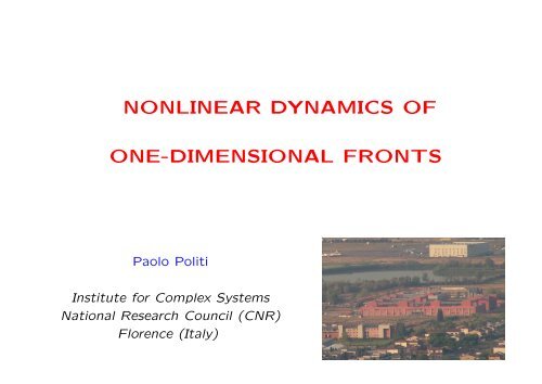
NONLINEAR DYNAMICS OF<br />
ONE-DIMENSIONAL FRONTS<br />
Paolo Politi<br />
Institute for Complex Systems<br />
National Research Council (CNR)<br />
Florence (Italy)
• Examples <strong>of</strong> experimental <strong>fronts</strong><br />
Outline <strong>of</strong> the lecture<br />
• Representative Partial Differential Equations and <strong>nonlinear</strong> behaviors<br />
• Linear stability analysis and relevant time/length scales<br />
• Multiple scales analysis (the anharmonic oscillator)<br />
• The amplitude and the phase equations
Meandering during Cu-MBE growth<br />
[T. Maroutian et al (CEA-Saclay). L = 640˚A]<br />
Fire propagation in paper<br />
[Zhang et al (Physica A, 1992). L = 8cm]<br />
Electromigration step-bunching on Si(111)<br />
[K. Sudoh (Osaka University)]<br />
Domain wall <strong>dynamics</strong> in Co film<br />
[Lemerle et al (PRL, 1998). L = 90µm]
Segregation <strong>of</strong> granular materials<br />
[SW Morris (Toronto University)]<br />
Fronts, but not only <strong>fronts</strong><br />
Rayleigh-Benard convection<br />
[S. Ciliberto et al (INO-Florence)]
Unstable growth <strong>of</strong> a high-symmetry surface<br />
Deposition, diffusion and nucleation,<br />
step-edge barriers<br />
∂th = F − ∂xJ<br />
J = A(∂xh) + K∂xxxh<br />
u(x, t) = ∂xh<br />
∂tu(x, t) = −∂xx[(δu − u 3 ) + uxx] = ∂xx<br />
F =<br />
Cahn-Hilliard equation<br />
<br />
dx<br />
1<br />
2 u2 x +<br />
<br />
−δ u2<br />
2<br />
<br />
u4<br />
+<br />
4<br />
δF<br />
δu<br />
<br />
dF<br />
dt<br />
= −<br />
<br />
dx<br />
<br />
∂x δF<br />
δu<br />
2<br />
≤ 0
Meandering <strong>of</strong> a single step<br />
Deposition, diffusion without nucleation,<br />
step-edge barriers and desorption<br />
∂u<br />
∂t = −δ∂2 u<br />
∂x2 − ∂4u + u∂u<br />
∂x4 ∂x<br />
Kuramoto-Sivashinsky equation<br />
F does not exist
Linear stability analysis<br />
Cahn − Hilliard ut = −∂xx[(δu − u 3 ) + uxx]<br />
Kuramoto − Sivashinsky ut = −δuxx − uxxxx + uux<br />
ω(q) = δq 2 − q 4<br />
u(x, t) = Aq(t) exp(iqx)<br />
ω<br />
0.3<br />
0<br />
Aq(t) = Aq(0) exp(ωt)<br />
q 2<br />
-0.3<br />
0 0.5 1<br />
q<br />
dAq<br />
dt = (δq2 − q 4 )Aq<br />
Modes with<br />
arbitrarily large λ<br />
are unstable
If translational invariance is broken . . .<br />
Swift − Hohenberg ut = δu − (1 + ∂xx) 2 u − u 3<br />
ω(q) = δ−(1−q 2 ) 2<br />
ω<br />
0.4<br />
0.2<br />
0<br />
-0.2<br />
-0.4<br />
q 1<br />
q c<br />
0 0.5 1 1.5 2<br />
q<br />
q 2 Only a band<br />
<strong>of</strong> finite q<br />
is unstable
t → ω0t ω0 =<br />
¨x + x = −ɛx 3<br />
Naive perturbation theory<br />
m¨x + kx = −k3x 3 Anharmonic (quartic) oscillator<br />
<br />
k<br />
m<br />
ɛ = k3<br />
k<br />
V (x) = x2<br />
2<br />
+ ɛx4<br />
4<br />
x = x0 + ɛx1 + . . . x0 = A cos(t + ϕ)<br />
¨x1 + x1 = −x 3 0 = −A3 cos 3 (t + ϕ) = −A 3 1 3 cos 3(t + ϕ) + 3 4<br />
x1(t) = − A3<br />
16<br />
sin(t + ϕ)(6t + sin 2(t + ϕ))<br />
⇑<br />
secular<br />
term<br />
cos(t + ϕ)<br />
⇑<br />
resonant<br />
forcing
¨x + x = −ɛx 3<br />
x = x0 + ɛx1 + . . .<br />
t0 = t, t1 = ɛt, . . .<br />
∂ 2 x0<br />
∂t 2 0<br />
d<br />
dt<br />
Multiple scales method<br />
= ∂<br />
∂t0<br />
+ ɛ ∂<br />
∂t1<br />
+ . . .<br />
+ x0 = 0 x0 = A0(t1) cos(t0 + ϕ0(t1))<br />
∂ 2 x1<br />
∂t 2 0<br />
+ x1 = −2 ∂2 x0<br />
∂t0∂t1<br />
= 2 dA0<br />
dt1<br />
− x 3 0<br />
dϕ0<br />
sin(t0 + ϕ0) + 2A0<br />
dt1<br />
d2 ∂2<br />
dt2 =<br />
∂t2 0<br />
+ 2ɛ ∂2<br />
∂t0∂t1<br />
− 3<br />
4 A3 0 cos(t0 + ϕ0)<br />
− A3 0<br />
4 cos(3(t0 + ϕ0))
Resonant forcing can be eliminated<br />
dϕ0<br />
2A0<br />
dt1<br />
x0(t0, t1) = A0 cos<br />
dA0<br />
dt1<br />
= 0 ⇒ A0 ≡ constant<br />
− 3<br />
4 A3 0 = 0 ⇒ ϕ0(t1) = 3<br />
8 A2 0 t1<br />
<br />
x0(t) = A0 cos<br />
t0 + 3<br />
8 A20 t1<br />
<br />
<br />
1 + 3<br />
8 A20 ɛ<br />
<br />
t<br />
We can continue with x1(t) and higher order terms. . .<br />
t0 = t, t1 = ɛt
ω(q) = δ − (q − 1) 2<br />
≡ ɛ 2 − (q − 1) 2<br />
ω<br />
0.4<br />
0.2<br />
0<br />
-0.2<br />
-0.4<br />
The amplitude equation<br />
q 1<br />
q c<br />
q 2<br />
0 0.5 1 1.5 2<br />
q<br />
q = 1 + k ω(k) = ɛ 2 − k 2 k = ɛQ, ω = ɛ 2 Ω Ω = 1 − Q 2<br />
e Ωt e iqx = e Ωɛ2 t e i(1+ɛQ)x = e ΩT e iQX e ix<br />
If T = ɛ 2 t and X = ɛx<br />
∂A<br />
∂T = A + ∂2A + <strong>nonlinear</strong> terms<br />
∂X 2<br />
u(x, t) = A(X, T )e ix + c.c.
The Ginzburg-Landau equation<br />
∂A<br />
∂T = A + ∂2 A<br />
∂X 2 − |A|2 A A → Ae iα<br />
Steady states: As(X) = A0e iQX 1 − A 2 0 − Q2 = 0<br />
As(X) =<br />
<br />
1 − Q 2 e iQX<br />
What about the stability <strong>of</strong> these solutions? (Secondary instability)
∂A<br />
∂T = A + ∂2 A<br />
∂X 2 − |A|2 A As(X) = A0e iQX<br />
A(X, T ) = A0(1 + r)e i(QX+φ)<br />
∂r<br />
∂T = −2A20 r + ∂2r ∂φ<br />
− 2Q<br />
∂X 2 ∂X<br />
∂φ ∂r<br />
= 2Q<br />
∂T ∂X + ∂2φ ∂X 2<br />
Adiabatic elimination procedure . . .
∂r<br />
∂T = −2A20 r + g(T )<br />
If g(T ) is slowly varying on the scale T ∗ = 1<br />
2A 2 0<br />
∂r<br />
∂T = −2A2 0 r + <br />
∂ 2 r<br />
<br />
∂X<br />
∂φ<br />
∂T = D ∂2 φ<br />
∂X 2<br />
Q 2 < 1 3<br />
Q 2 > 1 3<br />
<br />
<br />
<br />
2 − 2Q ∂φ<br />
∂X<br />
,<br />
∂r<br />
∂T<br />
= 0<br />
1<br />
= 0 ⇒ r ≈ −<br />
A2 Q<br />
0<br />
∂φ<br />
∂X<br />
D = 1 − 2Q2<br />
A 2 0<br />
D > 0 Stability<br />
= 1 − 3Q2<br />
A 2 0<br />
D < 0 Eckhaus Instability
Swift-Hohenberg<br />
equation<br />
Cahn-Hilliard type<br />
equation<br />
ω<br />
ω<br />
0.3<br />
0<br />
0.4<br />
0.2<br />
0<br />
-0.2<br />
-0.4<br />
q 1<br />
q c<br />
q 2<br />
0 0.5 1 1.5 2<br />
q<br />
-0.3<br />
0 0.5 1<br />
q<br />
creation elimination<br />
<strong>of</strong> rolls <strong>of</strong> rolls
∂φ<br />
∂T = D ∂2φ ∂X 2<br />
The phase diffusion coefficient<br />
D =<br />
1 − 3Q2<br />
A 2 0<br />
A 2 0<br />
(1 − 3Q 2 ) = d<br />
dQ (Q − Q3 ) = d<br />
dQ (QA2 0 )<br />
In many cases, D = [positive D0] ×<br />
= 1 − Q2<br />
d I(q)<br />
• The phase is stable/unstable if I is an increasing/decreasing function<br />
• The relation D ∼ λ2<br />
t<br />
gives the coarsening exp<strong>one</strong>nt<br />
dq
Ali Hasan Nayfeh<br />
Introduction to perturbation techniques<br />
Wiley-VCH<br />
Paul Manneville<br />
Instabilities, chaos and turbulence<br />
Imperial College Press<br />
Rebecca Hoyle<br />
Pattern formation<br />
Cambridge University Press