IMF Technical Memorandum #3 - Cramer Fish Sciences

S.P. Cramer & Associates, Inc.
IMF Technical Memorandum #3
To:
From: Steve Cramer
Zach Hymanson; Brent Walthall; Tim Quinn; Steve Macaulay;
Steve Cramer; Sam Luoma; Russ Bellmer; 'Ronald M. Yoshiyama';
Roger Guinee; Rick Sitts; Richard Denton; Paul Devries; Paul
Cadrett; Pat Brandes; Michael. E. Aceituno; Michael Carlin; Lisa
Holm; Lisa Culjis; Laura KingMoon; Kim Taylor; John Coburn; Joe
Miyamoto; Pat Coulston; Jim White; Jim Smith; Elaine Archibald;
Dudley Reiser; Doug Wallace; Doug Demko; Diana Jacobs; David
Harlow; Dan Odenweller; Chuck Armor; Bruce Oppenheim; Alice
Low
CC: Pat Brandes; Randy Brown
Date: January 28, 2004
Testing the Winter-run Chinook Model:
Smolt Survival Through the Delta
Introduction
This is the third Technical Memorandum to explain how we applied
historical data to test how well past trends in spawner abundance of winter-run
Chinook could be predicted by the Integrated Modeling Framework (IMF). The
first memorandum related to historical spawner abundance and egg survival, and
the second related to historical harvest rates. This memorandum describes our
derivation of estimates since 1968 for juvenile survival during migration through
the Delta. This is an important life stage to model for two reasons: 1) Delta
survival is highly variable, and 2 ) many factors affecting that survival are human
caused. Average survival of juvenile winter-run Chinook passing through the
Delta has not been directly estimated by sampling in any year, so we needed to
develop a means of accounting for variation in this survival when attempting to
predict historical population trends. We will discuss the data and methods used,
as well as their limitations.
What Factors Affect Survival Through the Delta?
There has been much analysis of factors influencing survival of juvenile fallrun
Chinook passing through the Delta, but little on juvenile winter-run Chinook
that pass in a different season and at a larger size. Accordingly, we derived our
approach from studies with juvenile fall-run Chinook, and assumed they were
applicable to winter-run chinook. We corroborated the reasonableness of that
Testing the Winter-run Chinook Model 1/30/2004 Page 1 of 18

S.P. Cramer & Associates, Inc.
assumption by comparing our results against those of Brandes (2003), who used
data from tests during late fall and winter with coded-wire-tagged (CWT) juvenile
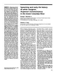
Chinook near the Delta Cross Channel (DCC; see map in Figure 1).
The most comprehensive analyses of data on factors affecting juvenile
Chinook survival through the Delta have been those of Newman and Rice (1997)
and Newman (2000). These works were later published as Newman and Rice
(2002) and Newman (2003).
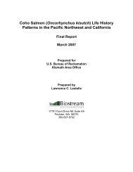
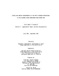
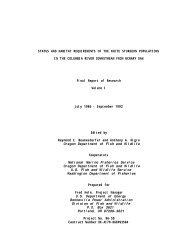
Figure 1. Map of the lower Sacramento River and Delta.
Testing the Winter-run Chinook Model 1/30/2004 Page 2 of 18

S.P. Cramer & Associates, Inc.
Newman and Rice (1997) analyzed survival estimates from CWT recoveries
of fall Chinook released above and below the DCC each spring between 1979
and 1995. They found that temperature was the most influential environmental
variable related to survival. Their work also indicated that flow, DCC gate
position, and export-to-inflow ratios may also influence Delta migration survival,
but those relationships were not statistically significant.
The work of Newman (2000) improved on the work of Newman and Rice
(1997) in estimating Delta survival and further isolated factors correlated with
survival. Newman and Rice (1997) conducted their analyses on trawl recoveries
at Chipps Island of CWT-marked Chinook, and used catch/fish released as an
index of survival. Thus, variation in trawl efficiency would have added error to
the index. Newman (2000) advanced the analysis by directly estimating Delta
survival from recoveries of paired CWT groups: groups released at the entry to
the Delta were paired with groups released at the exit to the Delta. The paired
analysis of Newman (2000) estimated survival through the Delta as a function of
the difference in ocean recovery rates for fish released in the river near
Sacramento compared to those released at Port Chicago or Benicia (Figure 1).
Newman (2000) found that the majority of cases in which estimated survival was
near 100%, flows exceeded 15,000 cfs and in all cases occurred only when
release temperatures were less than about 65° Fahrenheit. In further analysis on
the effects of covariates on survival Newman (2000) found:
“Flow effect can be seen to have the largest effect: as flow increases from
600 cfs to 15,000 cfs, survival increases from 0.37 to 0.67. The release
temperature effect is sizeable as well, with 40% decrease in survival as
temperature increase from 58 to 76 degrees Fahrenheit. At a moderate flow
of 8,100 cfs, the export effects are also sizeable. As export/inflow increases
from zero to 49% (within the historical range of export/inflow values when
flow was around 8,100 cfs), survival rate declines 22%. The effect of the
cross-channel gate being open is estimated to be roughly 18% decline in
survival.”
Newman (2003) compared results of his paired analysis with that of the
earlier unpaired analysis (Newman and Rice 1997). He found that the positive or
negative effect of each of the variables was similar between the two analyses,
but the significance of each relationship was consistently stronger for the paired
analysis. Flow had the strongest association with survival in the paired model,
whereas temperature had the strongest effect in the unpaired model.
Temperature still had a significant negative effect on survival in the paired model,
but the magnitude of the effect was less. The effect of the exports was greater in
the paired model.
In his final analysis of paired CWT releases, Newman (2003) compared
three statistical techniques for estimating environmental effects on survival, and
concluded the hierarchical formulation was the most reliable. Thus, we used his
hierarchical formulation in our modeling. Newman (2003) estimated coefficients
for a number of factors that might affect smolt survival, but we used those factors
Testing the Winter-run Chinook Model 1/30/2004 Page 3 of 18

S.P. Cramer & Associates, Inc.
pertinent to our analysis and that had statistically significant effects on survival.
Those factors for which we included coefficients estimated by Newman (2003)
were: river inflow, river temperature, exports, DCC gate position, turbidity, and
salinity (Table 1). Newman (2003) also found significant reductions in survival for
fish released upstream at Sacramento rather than at Ryde, but we did not include
this effect because the juvenile production (JPE) portion of our model already
predicted survival to the point of Delta entry (JPE averages survival estimates
from Battle Creek to various points representing Delta entry; Sacramento to
Ryde). We also did not include the effect of size, because Newman (2003)
showed that estimates of that coefficient changed substantially between model
formulations.
The equation we used to estimate survival through the Delta, based on
coefficients estimated by Newman (2003) is as follows:
Survival = -1.02 + 0.56*loge (Flow) – 0.56*River Temp. – 0.21*Exports +
0.04*Turbidity + 0.23*Salinity – 0.60*Gate Position
Where:
Flow = Mean flow in cubic feet per second at Freeport.
River Temp. = Mean temperature in Fahrenheit at Freeport
Export flow = Combined export flow to the State and Federal pumps
Turbidity = Turbidity of river in formazine turbidity units near Courtland
Salinity = water salinity measured by conductivity, µmho/cm at
Collinsville
Gate Position = Average of daily positions of the Delta Cross channel gates
where each day a value of 0 or 1 signaled both gates closed
or open, respectively.
Newman (2003) standardized all variables except the DCC position indicator
using the following equation:
Standardized Value = (Observation – Mean)/Standard Deviation
The mean and standard deviations for each variable were those reported by
Newman (2003) from the observations in the dataset for paired CWT releases.
Testing the Winter-run Chinook Model 1/30/2004 Page 4 of 18

S.P. Cramer & Associates, Inc.
Table 1. Coefficients for environment variables used to estimate winter-run Chinook Delta
survival. Relationship presented is the hierarchical formulation in Table 5 of
Newman (2003). These coefficients estimate the logistic transform of survival.
Coefficients of all variables except the gate indicator are for standardized
variables.
Covariate ß SE
Intercept -1.02 0.10
loge (River Flow) 0.56 0.09
River Temperature °F -0.56 0.07
Export Flow -0.21 0.07
Turbidity 0.04 0.10
Salinity 0.23 0.07
Gate Position Indicator -0.60 0.13
The equation we used includes salinity, which Newman (2003) reported
was highly correlated to flow (r = -0.79). Although the two variables are
negatively correlated, they both have a positive effect on survival (coefficients are
positive). The combination of these effects results in a non-linear relationship
between predicted survival and flow, because increasing flow reduces salinity,
which decreases the benefit of flow to survival. We determined the relationship
between salinity and flow by regressing salinity at Collinsville since 2000, and
Sacramento River inflow at Freeport. The data set was limited to observations
taken between December and March, because this is the primary time period
when winter Chinook pass through the Delta. There was a strong negative
exponential decline in salinity as flow increased (p

Salinity at Collinsville (micro ohms)
S.P. Cramer & Associates, Inc.
12000
10000
8000
6000
4000
2000
0
Relationship of Sacramento River Flow to Salinity
y = 102,003*e (-0.0002*x)
r 2 = 0.65
0 20 40 60 80 100
Flow at Freeport (1000s cfs)
Figure 2. Relationship between Sacramento River flow and salinity in the Delta.
How do the different variables drive the survival estimates?
We analyzed the sensitivity of Delta survival estimates to
environmental variables by varying one factor at a time. We examined the
ranges for each variable that corresponded to the ranges in the dataset of
Newman (2003). When we varied flow in this analysis, we concurrently
changed salinity according to the equation presented in Figure 2. The
sensitivity of temperature was not examined, because all temperatures in
Newman’s (2003) data set exceeded the range of temperatures that
juvenile winter-run Chinook will encounter when passing through the Delta
in December through March. The lowest temperature in the dataset of
Newman was 58 o F, which is near the upper boundary for optimal growth of
juvenile Chinook in a natural setting. Thus, the dataset analyzed by
Newman includes temperatures that ranged from the incipient lethal level in
the mid 70 o ’s F, down to the optimum range for growth. There is little
reason to expect that survival would continue to increase as temperature
declined below 58 o F, given that this within the optimum range for growth.
Therefore, we assumed there was no further benefit to smolt survival as
temperature dropped below 58 o F (i.e. we assumed the temperature effect
was the same as that at 58 o F).
The effects of each of the variables on the estimated Delta survival
Testing the Winter-run Chinook Model 1/30/2004 Page 6 of 18

S.P. Cramer & Associates, Inc.
can be seen in Figure 3. The most interesting result was the influence of
flow and salinity on survival. As flow increases from a minimum of 6,000
cfs to 15,000 cfs survival decreases. Though flow has a positive effect on
survival, increasing flow results in a decrease in salinity. Reductions in
salinity cause decreases in survival. Only up to 15,000 cfs, do the effects of
decreasing salinity out weight the positive effects of increasing flow.
Salinity drops to near zero at flows above 20,000 cfs, and survival benefits
of increasing flow begin to outweigh the effects of decreasing salinity at
approximately 15,000 cfs. The relationships of the other variables to
survival, as described by the Newman equation, are linear.
Estimated Survival
Estimated Survival
70%
60%
50%
40%
30%
70%
60%
50%
40%
30%
0 20,000 40,000 60,000
Flow (cfs)
5 10 15
Turbidity
20 25
0 2000 4000 6000 8000 10000
Exports (cfs)
0 0.2 0.4 0.6 0.8 1
Gate Position
Figure 3. Change in Delta survival predicted by the adapted Newman function used in the
IMF. One variable was varied while others were held at their mean value
observed during paired releases of CWTs analyzed by Newman (2003). The
effect of flow includes a link of flow to salinity according to the equation in
Figure 1.
Testing the Winter-run Chinook Model 1/30/2004 Page 7 of 18

S.P. Cramer & Associates, Inc.
The survival equation just described requires for any simulation that
values for environmental variables be supplied for the time frame when
juvenile winter-run Chinook pass through the Delta. Because timing of
peak migration varied between years, we next needed to account for
differences in timing of winter-run smolt passage through the Delta each
year.
When is Peak Migration Through the Delta?
Two peaks in outmigration of winter-run Chinook have generally
been apparent each year since 1995-96 from captures of juveniles in the
screw traps at Knights Landing, the trawl net at Sacramento, and the trawl
net at Chipps Island (Figure 4). In each year, the first significant peak in
passage followed the first major increase in flow during late-fall, generally in
November or December. Regardless of flow changes, migration also
consistently peaked a second time in March or early April, which we
assume corresponds to the peak timing of the physiological transition from
parr to smolt (seawater adaptation).
How was Survival of Two Migration Groups Modeled?
We accounted for the dual emigration peak in our test simulation of
historic conditions by predicting survival for both groups, and averaging the
survivals of those two groups. This was equivalent to assuming that half of
the smolts passed following the first peak in flow, and the other half passed
in March. The true pattern of emigration would have varied substantially
from this assumption, but we have yet to develop a more accurate method
of predicting smolt migration timing. Timing of passage at Sacramento has
only been monitored since 1995-96, so migration timing in prior years was
predicted from flows measured at Freeport. We assumed that migration
patterns between 1968 and 1994 were similar to those of 1995-2002, in that
there would have been a spike in migration following the first peak flow of
the season. Passage data during 1995-2002 showed that the initial spike in
migration each season lasted between 5 and 18 days following the first
peak flow. Consistent with that duration, we predicted survival during the
first peak in migration by using the mean values for environmental variables
during the 10 days following the first sharp increase in flow. Survival during
the second peak in migration that was typically in March [please show the
data that make these two emigration periods apparent to everyone] was
predicted using means for environmental variables during the full month of
March each year.
Testing the Winter-run Chinook Model 1/30/2004 Page 8 of 18

Cumulative Number Recovered
Cumulative Number Recovered
Cumulative Number Recovered
300
250
200
150
100
50
0
80
60
40
20
0
120
90
60
30
0
S.P. Cramer & Associates, Inc.
Number Recovered
Number Recovered
Number Recovered
NUMBER OF OLDER JUVENILE CHINOOK MEASURED IN THE
SACRAMENTO RIVER MIDWATER AND KODIAK TRAWLS
50
40
30
20
10
0
50
40
30
20
10
0
50
40
30
20
10
0
1995/1996
1 16 1 16 1 16 1 16 1 16 1 16 1 15 1 16 1 16 1 16 1 16 1 16 31
AUG 95 SEP 95 OCT 95 NOV 95 DEC 95 JAN 96 FEB 96 MAR 96 APR 96 MAY 96 JUN 96 JUL 96
1996/1997
1 16 1 16 1 16 1 16 1 16 1 16 1 15 1 16 1 16 1 16 1 16 1 16 31
AUG 96 SEP 96 OCT 96 NOV 96 DEC 96 JAN 97 FEB 97 MAR 97 APR 97 MAY 97 JUN 97 JUL 97
1997/1998
1 16 1 16 1 16 1 16 1 16 1 16 1 15 1 16 1 16 1 16 1 16 1 16 31
AUG 97 SEP 97 OCT 97 NOV 97 DEC 97 JAN 98 FEB 98 MAR 98 APR 98 MAY 98 JUN 98 JUL 98
Figure 4. Example of two peaks in outmigration of winter-run-sized Chinook (bars) captured in the
Sacramento trawl during winter. Figures from Erin Chappell, DWR, Sacramento.
Testing the Winter-run Chinook Model 1/30/2004 Page 9 of 18
100
80
60
40
20
0
120
100
80
60
40
20
0
100
80
60
40
20
0
Freeport Flows cfs*1000
Freeport Flows cfs*1000
Freeport Flows cfs*1000
25
20
15
10
5
0
25
20
15
10
5
0
25
20
15
10
5
0
Water Temperature (C)
Water Temperature (C)
Water Temperature (C)

S.P. Cramer & Associates, Inc.
Although river temperature was a key factor relating to passage
survival in the data analyzed by Newman (2003), river temperatures during
winter are nearly always lower than the lowest value (58°F) in the data set
for fall Chinook used by Newman. Newman (2003) found that passage
survival increased as river temperature decreased from 70°F to 58°F. It is
doubtful that survival would have increased further as temperature dropped
below 58°F, so we assumed the temperature effect at

S.P. Cramer & Associates, Inc.
Table 2. Values for environmental variables used to predict Delta survival of winter-run Chinook smolts during the
first peak (peak flow passage) and second peak (March) in outmigration, 1968-2002. Temperature was
assumed to be less than 58ºF in all instances. “Peak” and “March” values are 10 and 31-day averages,
respectively.
Run Peak Flow Passage Conditions March Conditions
Total
Year Start 10 days Frpt. Q Exports Gates Salinity Turbidity Survival Survival Frpt. Q Exports Gates Salinity Turbidity Survival Survival
1968-69 12-Dec 25,270 2,952 0.5 517 8.2 0.25 0.56 49,730 3,403 0.0 235 8.2 0.79 0.68
1969-70 13-Dec 29,810 1,102 0.0 221 8.2 0.92 0.71 44,210 2,265 0.2 158 8.2 0.76 0.74
1970-71 19-Nov 24,870 2,049 0.0 167 8.2 0.59 0.64 30,480 4,702 0.4 187 8.2 0.59 0.62
1971-72 23-Dec 27,550 1,497 0.5 212 8.2 0.48 0.62 23,900 6,601 0.7 172 8.2 0.42 0.52
1972-73 11-Nov 22,160 3,623 0.5 275 8.2 0.00 0.50 51,640 1,331 0.0 243 8.2 0.83 0.66
1973-74 8-Nov 44,350 5,014 0.5 327 8.2 0.73 0.68 64,680 6,200 0.0 140 8.2 0.80 0.74
1974-75 11-Nov 20,720 1,829 1.0 161 8.2 -0.21 0.45 50,940 6,061 0.2 172 8.2 0.73 0.59
1975-76 11-Nov 21,500 7,842 1.0 190 8.2 -0.75 0.32 14,570 8,410 1.0 2,224 8.2 0.24 0.28
1976-77 1-Jan 10,625 6,568 1.0 6,830 8.2 -1.10 0.25 6,573 3,724 1.0 7,281 8.2 0.20 0.22
1977-78 16-Dec 17,270 8,664 1.0 7,595 8.2 -0.65 0.34 55,570 5,773 0.2 194 8.2 0.75 0.55
1978-79 11-Jan 36,320 4,236 0.2 711 8.2 0.76 0.68 29,170 4,386 0.0 199 8.2 0.63 0.66
1979-80 24-Dec 36,870 6,430 0.2 475 8.2 0.55 0.63 55,340 4,441 0.0 203 8.2 0.80 0.72
1980-81 4-Dec 21,600 6,647 1.0 963 8.2 -0.58 0.36 24,510 4,862 0.0 254 8.2 0.58 0.47
1981-82 12-Nov 29,246 5,064 0.3 5,414 8.2 0.64 0.66 62,810 10,410 0.0 159 8.2 0.72 0.69
1982-83 18-Nov 41,510 5,231 0.0 127 8.2 0.92 0.71 78,290 5,429 0.0 189 8.2 0.84 0.78
1983-84 11-Nov 52,120 925 0.3 161 8.2 1.44 0.81 31,430 6,905 0.0 202 8.2 0.60 0.71
1984-85 8-Nov 23,580 8,186 0.6 677 8.2 -0.40 0.40 14,310 8,599 0.5 575 8.2 0.26 0.33
1985-86 24-Nov 17,400 9,460 0.7 6,445 8.2 -0.61 0.35 74,980 3,219 0.0 194 8.2 0.86 0.61
1986-87 4-Jan 15,200 6,290 0.0 1,523 8.2 -0.35 0.41 21,580 5,596 0.2 418 8.2 0.49 0.45
1987-88 3-Dec 19,150 7,005 1.0 6,984 8.2 -0.40 0.40 11,350 8,479 1.0 5,791 8.2 0.22 0.31
1988-89 24-Nov 17,240 8,795 0.9 4,580 8.2 -0.79 0.31 43,370 10,288 0.2 1,881 8.2 0.61 0.46
1989-90 21-Oct 16,960 10,643 1.0 6,089 8.2 -0.96 0.28 12,870 10,611 1.0 5,279 8.2 0.21 0.24
1990-91 none -- -- -- -- -- -- -- 25,760 9,794 0.3 2,975 8.2 0.47 0.47
1991-92 6-Jan 13,346 8,611 1.0 7,205 8.2 -0.99 0.27 20,340 10,490 0.0 326 8.2 0.38 0.33
1992-93 9-Dec 20,340 2,890 0.9 5,364 8.2 0.04 0.51 49,340 6,117 0.0 268 8.2 0.74 0.63
1993-94 7-Dec 23,860 10,686 1.0 5,272 8.2 -0.59 0.36 13,460 4,311 0.0 459 8.2 0.41 0.38
1994-95 4-Dec 20,660 6,132 0.5 4,782 8.2 -0.05 0.49 71,920 2,956 0.0 226 8.2 0.86 0.67
1995-96 18-Dec 31,820 4,360 0.0 148 8.2 0.67 0.66 56,240 3,677 0.0 136 8.2 0.81 0.74
1996-97 10-Dec 69,000 8,320 0.0 131 8.2 1.25 0.78 24,470 7,132 0.0 202 8.2 0.52 0.65
1997-98 24-Nov 22,400 10,785 0.2 5,493 8.2 -0.19 0.45 63,830 2,507 0.0 262 8.2 0.85 0.65
1998-99 23-Nov 33,680 1,654 0.0 134 8.2 1.01 0.73 56,840 7,223 0.0 167 8.2 0.75 0.74
1999-00 11-Jan 18,410 9,146 0.6 4,522 8.2 -0.57 0.36 58,560 9,152 0.0 171 8.2 0.72 0.54
2000-01 9-Jan 19,190 4,496 0.6 5,658 8.2 0.01 0.50 24,700 7,932 0.0 301 8.2 0.50 0.50
2001-02 24-Nov 19,690 5,291 0.5 5,563 8.2 0.02 0.50 21,320 8,276 0.0 317 8.2 0.45 0.48
2002-03 14-Dec 41,831 10,058 0.3 2,917 8.2 0.44 0.61 22,960 10,855 0.0 289 8.2 0.41 0.51
Testing the Winter-run Chinook Model 1/30/2004 Page 11 of 18

S.P. Cramer & Associates, Inc.
How do conditions during the paired CWT experiments analyzed by Newman
compare to those during migration of winter-run smolts?
The current Delta survival function used in the IMF was developed using paired
CWT release groups of fall-run Chinook. Though this method uses the best available
data on smolt survival through the Delta, environmental conditions during emigration of
fall-run Chinook generally differ from those during emigration of winter-run Chinook.
Some parameters applied in the winter Chinook model are outside the range of
observations used by Newman (2003). Because of our concern for predicting survival
when environmental factors were outside the range of values analyzed by Newman, we
examined the frequency with which winter conditions fell outside the range of analyzed
data. We compared frequency distributions for environmental variables in the dataset
analyzed by Newman to those for the period of Delta passage by winter-run Chinook
smolts during 1968-2001. These comparisons were precautionary, to help us
understand the extent that conditions for which we were predicting survival overlapped
with the conditions used to develop the prediction function.
Sacramento River Flow
Sacramento River flow at Freeport during emigration of CWT groups evaluated
by Newman (2003) ranged from 6,085 to 50,800 cubic feet per second (cfs). The
frequency distribution of flow data indicates that CWT groups were generally released at
flows between 5,000 and 15,000 cfs, with most at flows of 12,500 to 15,000 cfs (Figure
6). Few CWT groups were released at flows greater than 35,000 cfs (Figure 6), so the
predicted increases in survival related to flows above 35,000 cfs should be accepted
with caution. About one third of historic flows during winter-run smolt passage were
greater than 35,000 cfs (Figure 4). We regard the survival effects of flow above 35,000
as a critical uncertainty that needs testing.
% of Observations
45%
40%
35%
30%
25%
20%
15%
10%
5%
0%
Frequency Distribution of Flow Values
2,500
7,500
12,500
17,500
25,000
35,000
45,000
55,000
65,000
75,000
85,000
Testing the Winter-run Chinook Model 1/30/2004 Page 12 of 18
Flow
Newman
Hindcast
Figure 6. Frequency distributions of Sacramento River flows during the CWT releases analyzed
by Newman (2003) compared to those used to predict historic values of Delta survival for
winter-run Chinook smolts during 1968-2001.

S.P. Cramer & Associates, Inc.
Water Temperature
Water temperatures during the paired CWT releases analyzed by Newman
(2003) ranged from 58°F to 76°F, while water temperatures during winter-run emigration
(November through March) were nearly always

S.P. Cramer & Associates, Inc.
% of Observations
25%
20%
15%
10%
5%
0%
Frequency Distribution of Export Values
1,000
2,000
3,000
4,000
5,000
6,000
7,000
8,000
9,000
10,000
11,000
Exports (cfs)
Newman
Hindcast
Figure 8. Frequency distribution of observed water export volumes in the dataset used by
Newman (2003) and those used to predict historic values of Delta survival for winterrun
Chinook smolts during 1968-2001.
Salinity
Salinity during emigration of CWT groups evaluated by Newman (2003) ranged
from 160-12,873 µmhos, and was most often less than 1,000 µmhos. The same held
true for historic values during outmigration of winter-run Chinook smolts. Thus, the
coefficient for salinity in Newman’s function (Table 1) should be appropriate for winterrun
Chinook.
% of Observations
70%
60%
50%
40%
30%
20%
10%
0%
Frequency Distribution of Salinity Values
1,000
2,000
3,000
4,000
5,000
6,000
7,000
8,000
9,000
10,000
11,000
12,000
13,000
Salinity (micro mohs)
Newman
Hindcast
Figure 9. Frequency distribution of observed salinity in the dataset used by Newman (2003) and
those used to predict historic values of Delta survival for winter-run Chinook smolts
during 1968-2001. X-axis labels give upper bound of interval.
Testing the Winter-run Chinook Model 1/30/2004 Page 14 of 18

S.P. Cramer & Associates, Inc.
Alternative Evidence for Predicting Delta Survival in the Winter
We checked the reliability of the Newman (2003) function for predicting Delta
survival in the winter by comparing its predictions to analyses and modeling of Brandes
(personal communication, USFWS, Stockton) that were based on field experiments at
the Delta Cross Channel (DCC) with late-fall-run Chinook during November to January.
CWT experiments to evaluate effects of the DCC have been conducted in the Delta
during November- January each winter since 1995. Data from those experiments
provided an opportunity to check how well the observed smolt survivals during winter fit
the predictions of the Newman equation, given the actual conditions that existed at the
time of the late-fall CWT experiments. The results of this comparison, as will be
described, indicate that the Newman equation can be used to predict survival through
the Delta in the winter.
Experimental releases of late-fall Chinook near the DCC in November through
January were not conducted so as to directly estimate overall of juvenile salmon
survival through the Delta from Sacramento to Chipps Island (as the Newman equation
does), but rather they provided ratios for expanded recovery rates in the Chipps Island
trawl of fish passing through Georgiana Slough versus those passing down the main
Sacramento River to Chipps Island. By making some simplifying assumptions, Pat
Brandes (USFWS) was able to use the GS/Ryde recovery ratio in a five-step model to
estimate survival from Sacramento to Chipps Island. Her model was based on the
assumptions that (a) the proportion of juveniles following migration routes through the
central Delta is equal to the proportion of Sacramento flow entering the central Delta,
and that (b) Delta survival of juveniles continuing down the main stem Sacramento
River to Chipps Island is constant at 80%. We compared the estimates from her model
to predictions from the Newman equation to see if the results corroborated each other.
The model by Brandes to estimate survival of juvenile Chinook migrating through
the Delta in winter used the following steps:
1. Because there was a limited number of tests performed with CWT groups, each
at a discrete flow, Brandes needed first to quantify how survival varied across the
continuous range of flows tested. To do this she regressed the GS/Ryde survival
ratio from late-fall experiments on the export rates averaged for three days after
release of each CWT group.
2. The regression in step 1 was then used to estimate the average GS/Ryde
survival ratio for a given winter based on the mean export level between
December 1 and April 15 that winter.
3. The proportion of smolts continuing down the main stem versus entering the
Central Delta was assumed equal to the proportions of flow passing those two
routes during the month of December.
4. The actual survival from Ryde to Chipps Island was assumed to be 80%, which is
in the range of direct estimates in the spring, as calculated by Newman (2003).
5. Given the values calculated in steps 1-4, the survivals for the Interior Delta route
Testing the Winter-run Chinook Model 1/30/2004 Page 15 of 18

S.P. Cramer & Associates, Inc.
could be calculated and survivals from the two routes could be combined to
estimate average survival through the Delta.
The equations and data used to complete the preceding five steps are described
in more detail here. Experiments using late fall hatchery fish from Coleman National
Fish Hatchery were used to estimate survival index ratios between fish migrating from
Ryde and through the mainstem Sacramento and Georgiana Slough migration through
the interior Delta. Brandes found that GS:Ryde survival index ratios were negatively
correlated to average exports three days after release of the experimental groups, as
defined by the equation:
GS:R = (3*10 -5 )*Exports + 0.4583
Where:
GS:R = Georgian Slough to Ryde survival index ratio
This relationship was subsequently used in the Brandes model to estimate Delta
migration survival via the equation:
S = (SM(PM) + SI(PI))/100
and
SI = (G:R)* SM
Where:
S = Survival index of all migrants
SM = Survival index of fish migrating through the mainstem (assumed to be 0.8)
SI = Survival index of fish migrating through the interior Delta
PM = Proportion of outmigrants migrating through the mainstem; assumed equal to the
proportion of flow not diverted from the mainstem in December.
PI = Proportion of outmigrants migrating through the interior Delta; assumed equal to the
proportion of flow diverted from the mainstem in December.
Brandes estimated Delta survival of late fall Chinook via this model using the percent of
water diverted in December and the mean exports between December 1 and April 15
for the migration years of 1995-96 to 2002-03. We compared the survival estimates of
Brandes to Delta survival as estimated via the Newman equation under the same
environmental conditions.
Survival estimates of the two methods were strongly and significantly correlated
(p

S.P. Cramer & Associates, Inc.
flow, export flow, and DCC gate position. The corroboration of the two models lends
support to assumptions made and relationships used within each model, and gives
added credence to their respective results.
Newman (2003) Survival
0.9
0.8
0.7
0.6
0.5
0.4
0.3
0.2
y = 2.45x - 1.09
R 2 = 0.76
1995-96 through 2002-03
0.55 0.60 0.65 0.70 0.75
Brandes Survival
Figure 10. Relationship between survival predictions by the methods of Brandes vs those of
Newman for winter-run Chinook smolts passing through the Delta during the winters of
1995-96 through 2002-03.
Table 3. Environmental values used in the Brandes and Newman models, and the associated
estimates of survival for winter-run Chinook smolts passing through the Delta.
Brandes Newman
Year % Diverted Survival Flow (cfs) Temp (F) Exports Gate Pos. Salinity Turbidity Survival
1995-96 26 0.66 24,570

S.P. Cramer & Associates, Inc.
Newman , K. 2000. Estimating and modeling survival rates for juvenile chinook salmon
outmigrating through the lower Sacramento River using paired releases.
Unpublished technical report for California Department of Water Resources.
Contract No. B-81353.
Newman, K. and J. Rice. 2002. Modeling the survival of chinook salmon smolts
outmigrating through the lower Sacramento River system. Journal of the
American Statistical Association, 97: 983-993.
Newman, K. 2003. Modelling paired release-recovery data in the presence of survival
and capture heterogeneity with application to marked juvenile salmon. Statistical
Modelling, 3: 157-177.
Testing the Winter-run Chinook Model 1/30/2004 Page 18 of 18