Lab 2: Exercises in Uncertainty
Lab 2: Exercises in Uncertainty
Lab 2: Exercises in Uncertainty
Create successful ePaper yourself
Turn your PDF publications into a flip-book with our unique Google optimized e-Paper software.
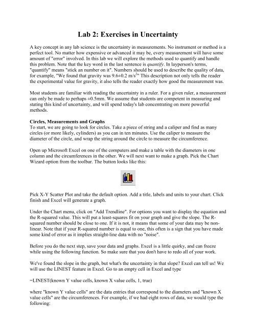
<strong>Lab</strong> 2: <strong>Exercises</strong> <strong>in</strong> Uncerta<strong>in</strong>ty<br />
A key concept <strong>in</strong> any lab science is the uncerta<strong>in</strong>ty <strong>in</strong> measurements. No <strong>in</strong>strument or method is a<br />
perfect tool. No matter how expensive or advanced it may be, every measurement will have some<br />
amount of "error" <strong>in</strong>volved. In this lab we will explore the methods used to quantify and handle<br />
this problem. Note that the key word <strong>in</strong> the last sentence is quantify. In layperson's terms,<br />
"quantify" means "stick an number on it". Numbers should be used to describe the quality of data,<br />
for example, "We found that gravity was 9.6±0.2 m/s 2 " This description not only tells the reader<br />
the experimental value for gravity, it also tells the reader exactly how good the measurement was.<br />
Most students are familiar with read<strong>in</strong>g the uncerta<strong>in</strong>ty <strong>in</strong> a ruler. For a given ruler, a measurement<br />
can only be made to perhaps ±0.5mm. We assume that students are competent <strong>in</strong> measur<strong>in</strong>g and<br />
stat<strong>in</strong>g this k<strong>in</strong>d of uncerta<strong>in</strong>ty, and will spend today's lab concentrat<strong>in</strong>g on more powerful<br />
methods.<br />
Circles, Measurements and Graphs<br />
To start, we are go<strong>in</strong>g to look for circles. Take a piece of str<strong>in</strong>g and a caliper and f<strong>in</strong>d as many<br />
circles (or more likely, cyl<strong>in</strong>ders) as you can <strong>in</strong> ten m<strong>in</strong>utes. Use the caliper to measure the<br />
diameter of the circle, and wrap the str<strong>in</strong>g around the circle to measure the circumference.<br />
Open up Microsoft Excel on one of the computers and make a table with the diameters <strong>in</strong> one<br />
column and the circumferences <strong>in</strong> the other. We will next want to make a graph. Pick the Chart<br />
Wizard option from the toolbar. The button looks like this:<br />
Pick X-Y Scatter Plot and take the default option. Add a title, labels and units to your chart. Click<br />
f<strong>in</strong>ish and Excel will generate a graph.<br />
Under the Chart menu, click on "Add Trendl<strong>in</strong>e". For options you want to display the equation and<br />
the R-squared value. This will put a least-squares fit on your graph and give the slope. The Rsquared<br />
number should be close to one. If it is not, it means that some of your data may be nonl<strong>in</strong>ear.<br />
Note that if your R-squared number is equal to one, this often is a sign that you have made<br />
some k<strong>in</strong>d of error as it implies straight-l<strong>in</strong>e data with no "noise".<br />
Before you do the next step, save your data and graphs. Excel is a little quirky, and can freeze<br />
while us<strong>in</strong>g the follow<strong>in</strong>g function. So make sure that you don't have to redo all of your work.<br />
We've found the slope <strong>in</strong> the graph, but what's the uncerta<strong>in</strong>ty <strong>in</strong> that slope? Excel can tell us! We<br />
will use the LINEST feature <strong>in</strong> Excel. Go to an empty cell <strong>in</strong> Excel and type<br />
=LINEST(known Y value cells, known X value cells, 1, true)<br />
where "known Y value cells" are the data entries that correspond to the diameters and "known X<br />
value cells" are the circumferences. For example, if we had eight rows of data, we would type the<br />
follow<strong>in</strong>g:
=LINEST(B1:B8, A1:A8, 1, true)<br />
When we type this <strong>in</strong> Excel will return a s<strong>in</strong>gle value, the slope. LINEST is an array function,<br />
which means that even though it is try<strong>in</strong>g to give back a lot of values, it only displays one per cell.<br />
What Excel is expect<strong>in</strong>g you to do is highlight a 2x2 set of cells with the LINEST formula <strong>in</strong> the<br />
upper-left cell. Once this is done, go up to the formula bar and highlight the entire LINEST<br />
equation you typed <strong>in</strong> and hit Ctrl-Shift-Enter (on a Mac use Apple-Return). This will fill <strong>in</strong> the<br />
2x2 square. Upper left will be the slope, lower left will be the uncerta<strong>in</strong>ty on the slope. Upper right<br />
will be the <strong>in</strong>tercept and lower right will be the uncerta<strong>in</strong>ty on the <strong>in</strong>tercept.<br />
A little reflection on circles will tell you exactly what the slope and <strong>in</strong>tercept should be. Do these<br />
true values fall <strong>in</strong>side your uncerta<strong>in</strong>ties?<br />
Repeated Measurements<br />
When a scientist performs an experiment, he or she will often do it multiple times. Why? Because<br />
repeated measurements allow for random measurement errors to cancel. The average (mean) of<br />
several measurements is almost always a better value than just one measurement. The reported<br />
value for your measurements will be the mean value. For students who need a refresher, the mean<br />
is the sum of all of the measurements, divided by the number of measurements.<br />
But what about a statement like "We found that gravity was 9.6±0.2 m/s 2 "? It was stated <strong>in</strong> the<br />
previous paragraph that more measurements implies a better estimate of the true value, how is that<br />
expressed <strong>in</strong> the statement of the measurement? It is reflected <strong>in</strong> the ±0.2 part. If we took more<br />
measurements, we could shr<strong>in</strong>k this number. Here we need to <strong>in</strong>troduce a concept known as the<br />
standard error.<br />
Many students know about the standard deviation from their statistics classes. A close relative is<br />
the sample standard deviation. It is def<strong>in</strong>ed as:<br />
σ = {[Σi (xmean - xi) 2 ]/(n-1) } 1/2<br />
Hard to follow? Well, let's take the follow<strong>in</strong>g numbers:<br />
18<br />
15<br />
22<br />
14<br />
8<br />
That totals to 77, so the mean value is 77/5 = 15.4, and to calculate the sample standard deviation<br />
we first need to sum the square of the differences:<br />
(18-15.4) 2 = 6.76<br />
(15-15.4) 2 = 0.16<br />
(22-15.4) 2 = 43.56<br />
(14-15.4) 2 = 1.96<br />
(8-15.4) 2 = 54.76<br />
That sums to 107.2, next we need to divide by the number of measurements - 1 and then take the<br />
square root. So our f<strong>in</strong>al value will be (107.2/4) 1/2 = 5. Why 5 rather than 5.177? Because
uncerta<strong>in</strong>ties are normally reported with only one sig fig (an exception is made for lead<strong>in</strong>g ones,<br />
hence 1.7 would be reported, even through it consists of two sig figs).<br />
So the ±0.2 part <strong>in</strong> the gravity measurement is the sample standard deviation, right? No, it is<br />
actually someth<strong>in</strong>g called the standard error. The standard error is the sample standard deviation<br />
divided by the square root of the number of measurements. In this case, the standard error would<br />
be 2 (2.3 for those of you who want to see the next digit). The standard error will give the proper<br />
scal<strong>in</strong>g for the reduced uncerta<strong>in</strong>ty for repeated measurements.<br />
At this po<strong>in</strong>t, you may feel like all this math makes you want to drop physics and change careers.<br />
These numbers are used so often that there is no need to calculate them by hand, just about any<br />
mathematics software will generate them for you. In Excel, enter one of the data sets <strong>in</strong>to a<br />
column. Then go to the Tools menu and select Data Analysis. This will open a box with many<br />
options. Choose Descriptive Statistics and click OK. This will open a new box which prompts for<br />
an <strong>in</strong>put range, select your column of data. For output options, choose Summary Statistics. Excel<br />
will then produce a set of numbers, the first is the mean, and the second is the standard error, the<br />
two quantities we want.<br />
Propagation of Error<br />
How do the uncerta<strong>in</strong>ties <strong>in</strong> the more basic measurements come <strong>in</strong>to play? For multiplication, we<br />
have a simple rule. We def<strong>in</strong>e the percentage uncerta<strong>in</strong>ty to be the uncerta<strong>in</strong>ty divided by the<br />
mean. In other words, for our gravity example we would take ±0.2 and divide by 9.6 to get a 2.1%<br />
percentage error. The percentage error <strong>in</strong> a product is the square root of the sum of the squares of<br />
the percentage errors. Aga<strong>in</strong>, that's too many words when a formula will do the job much better:<br />
±c/C = [ (±a/A) 2 + (±b/B) 2 ] 1/2<br />
The above formula assumes that C = AB, but it works the same way for C=A/B. Note that the<br />
rules are slightly different for exponents, the percentage uncerta<strong>in</strong>ty d 2 is actually twice the<br />
percentage uncerta<strong>in</strong>ty <strong>in</strong> d.<br />
The uncerta<strong>in</strong>ty <strong>in</strong> a sum roughly follows the uncerta<strong>in</strong>ty <strong>in</strong> a product <strong>in</strong> that we use a<br />
Pythagorean-style formula. For the uncerta<strong>in</strong>ty <strong>in</strong> a sum we would write:<br />
±c = [ (±a) 2 + (±b) 2 ] 1/2<br />
In other words we use the uncerta<strong>in</strong>ties themselves rather than the respective percentage<br />
uncerta<strong>in</strong>ties.<br />
In today's lab your <strong>in</strong>stuctor will give you three sets of numbers. These sets correspond to<br />
imag<strong>in</strong>ary measurements of quantities A, B and C. Calculate you answer for A by hand, and then<br />
use Excel to calculate B and C. When that is completed, use the error propagation techniques to<br />
calculate a value for C/(A+B).<br />
The Mean<strong>in</strong>g of Error Bars<br />
Statistics course spend a large amount of time on hypothesis test<strong>in</strong>g. In this class we will play a<br />
little "fast and loose" and claim that 68% of the time the true value falls with<strong>in</strong> the error bars.<br />
People familiar with the Guassian distribution will recognize that this means that 95% of the time
the true value is with<strong>in</strong> twice the value of the error bars, and 99.7% three times the value. Aga<strong>in</strong>,<br />
roughly speak<strong>in</strong>g, most shoot for the 95% mark. If we f<strong>in</strong>d that our value differs from the accepted<br />
value by more than twice the error bar, we are concerned as there is only a 5% chance that is due<br />
to some statistical fluke. Students should always reference there numbers with respect to the error<br />
bars <strong>in</strong> their discussions.<br />
We have covered many concepts <strong>in</strong> today's lab, and for most students many of them are new.<br />
While the methods for handl<strong>in</strong>g uncerta<strong>in</strong>ty are very important, we will come back to them<br />
aga<strong>in</strong> and aga<strong>in</strong> this quarter. Do not be discouraged if you don't feel that you have mastered<br />
them today, <strong>in</strong>stead treat today's exercises as an <strong>in</strong>troduction.


