Hot or Not: An Investigation of Attractiveness Distributions in Men ...
Hot or Not: An Investigation of Attractiveness Distributions in Men ...
Hot or Not: An Investigation of Attractiveness Distributions in Men ...

You also want an ePaper? Increase the reach of your titles
YUMPU automatically turns print PDFs into web optimized ePapers that Google loves.
Seth Zimmerman<br />
Chetan Mehta<br />
Math 50<br />
<strong>Hot</strong> <strong>or</strong> <strong>Not</strong>: <strong>An</strong> <strong>Investigation</strong> <strong>of</strong><br />
<strong>Attractiveness</strong> <strong>Distributions</strong> <strong>in</strong> <strong>Men</strong> and<br />
Women<br />
I. Introduction<br />
How do perceptions <strong>of</strong> male attractiveness differ from perceptions <strong>of</strong> female<br />
attractiveness? This paper addresses one aspect <strong>of</strong> that problem by attempt<strong>in</strong>g to<br />
determ<strong>in</strong>e whether and how the distribution <strong>of</strong> male attractiveness differs from the<br />
distribution <strong>of</strong> female attractiveness—i.e., if a man is selected at random, what are the<br />
chances he will fall with<strong>in</strong> a certa<strong>in</strong> attractiveness range, and how will those chances<br />
differ from the chances a woman will fall with<strong>in</strong> that same range? Intuitively, several<br />
answers to this question seem plausible. On one hand, it seems anecdotally to be true that<br />
there are few extremely attractive people, many average look<strong>in</strong>g people, and few<br />
extremely unattractive people. Such logic could lead one to predict a n<strong>or</strong>mal<br />
attractiveness distribution. On the other hand, one could also argue that there are two<br />
dist<strong>in</strong>ct prototypes f<strong>or</strong> people—an “attractive” prototype and an “unattractive” prototype.<br />
This reason<strong>in</strong>g might lead to a prediction <strong>of</strong> bimodality <strong>in</strong> the attractiveness distribution.<br />
The w<strong>or</strong>k here aims to see whether empirical analysis bears out either <strong>of</strong> these<br />
cognitively plausible models, <strong>or</strong> whether it suggests that a different process may be at<br />
w<strong>or</strong>k <strong>in</strong> either the male <strong>or</strong> the female case.<br />
Our <strong>in</strong>vestigation relies on a unique but somewhat compromised data source: the<br />
website www.hot<strong>or</strong>not.com. Users <strong>of</strong> this website rate pictures other users have posted <strong>of</strong><br />
themselves on 1-10 attractiveness scale, with one be<strong>in</strong>g the low end and ten the high end.<br />
The website then computes and displays the average sc<strong>or</strong>e each user has received, along<br />
with the total number <strong>of</strong> rat<strong>in</strong>gs the average is based on. With 75,000 pictures posted as<br />
<strong>of</strong> several years ago (http://www.hot<strong>or</strong>not.com/pages/about.html) and millions <strong>of</strong> votes<br />
cast <strong>in</strong> total, the site represents a potentially robust source <strong>of</strong> attractiveness data. It is<br />
clear, however, that the site’s audience may not be very representative <strong>of</strong> the population<br />
as a whole—it is restricted to computer users, who may tend to be younger than the<br />
general population, and it is most likely frequented by people who are m<strong>or</strong>e concerned<br />
with their appearances than the average person. These caveats, however, do not prevent<br />
the hot<strong>or</strong>not.com data from provid<strong>in</strong>g an <strong>in</strong>terest<strong>in</strong>g and convenient first look at<br />
perceptions <strong>of</strong> attractiveness <strong>in</strong> men and women.<br />
II. Data Collection<br />
We collected a sample <strong>of</strong> 250 male sc<strong>or</strong>es and 250 female sc<strong>or</strong>es. Imp<strong>or</strong>tantly, we<br />
ensured that each <strong>of</strong> these sc<strong>or</strong>es represented the average <strong>of</strong> at least 100 votes. This step<br />
was necessary to prevent the variance <strong>of</strong> the sc<strong>or</strong>es (which, as above, c<strong>or</strong>respond to
sample means <strong>of</strong> votes) from <strong>in</strong>terfer<strong>in</strong>g with our plot <strong>of</strong> “true” attractiveness values,<br />
which we assumed the “true” averages would represent.<br />
Establish<strong>in</strong>g a 100 vote m<strong>in</strong>imum allows f<strong>or</strong> the construction <strong>of</strong> a 95% confidence<br />
<strong>in</strong>terval <strong>of</strong> approximate width 1.75 even <strong>in</strong> an implausible w<strong>or</strong>st case scenario. S<strong>in</strong>ce the<br />
variance <strong>of</strong> a sc<strong>or</strong>e is equal to the variance <strong>of</strong> an <strong>in</strong>dividual vote, Y i<br />
, divided by the total<br />
number <strong>of</strong> votes (i.e., Var(Y _ ) 2 n , where 2 is the variance <strong>of</strong> an <strong>in</strong>dividual vote), the<br />
variance <strong>of</strong> the sc<strong>or</strong>e f<strong>or</strong> any person with at least 100 votes must be less than the variance<br />
<strong>of</strong> the sc<strong>or</strong>e f<strong>or</strong> a person with 100 votes, each <strong>of</strong> maximal variance. Clearly, the variance<br />
<strong>of</strong> an <strong>in</strong>dividual vote is maximized if it has a 50% chance <strong>of</strong> be<strong>in</strong>g a 1 and a 50% chance<br />
<strong>of</strong> be<strong>in</strong>g 10; i.e., f<strong>or</strong> each vote Y i , P(Y i =1) =.5 and P(Y i =10)=.5. Then, E(Y i )=5.5, and<br />
E(Y i 2 )=50.5. So, Var(Y i )= E(Y i 2 )- E(Y i ) 2 =50.5-30.25=20.25. Assume we have taken 100<br />
samples from a distribution with this w<strong>or</strong>st-case variance. Then, Var(Y _ )=20.25/100, and<br />
we can set up a 95% confidence <strong>in</strong>terval around Y _ , given that Y<br />
<br />
Var(Y)<br />
_<br />
and<br />
2* F (1.96) .95. Comput<strong>in</strong>g this <strong>in</strong>terval yields a range around Y_ with<br />
z<br />
approximate<br />
(total) width 1.76 with<strong>in</strong> which we can be 95% sure the real average value will fall. S<strong>in</strong>ce<br />
we do not <strong>in</strong>tend to evaluate the data us<strong>in</strong>g b<strong>in</strong> widths <strong>of</strong> less than one unit <strong>in</strong> width, a<br />
100 vote m<strong>in</strong>imum seems acceptable to ensure that our average values will not diverge by<br />
m<strong>or</strong>e than one b<strong>in</strong> from the underly<strong>in</strong>g true values—a precise enough fit to permit<br />
general distribution fitt<strong>in</strong>g, particularly given that it is almost impossible to imag<strong>in</strong>e a<br />
case that would even approach the maximum variance.<br />
III. Graphs, Data and Initial Observations
The relevant statistics f<strong>or</strong> the data:<br />
Male<br />
Female<br />
Mean 7.2572 6.36<br />
Variance 2.0083 3.6451<br />
Standard Deviation 1.417 1.9092<br />
N 250 250<br />
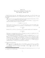
Even without the above <strong>in</strong>f<strong>or</strong>mation, a glance at the histograms reveals differences <strong>in</strong> the<br />
data f<strong>or</strong> men and women. The amount <strong>of</strong> data collected at the lower end <strong>of</strong> the<br />
distribution is small compared to the upper end. In addition, both histograms fav<strong>or</strong> a bimodal<br />
distribution – the female data m<strong>or</strong>e so than the male data – but s<strong>in</strong>ce we had little<br />
experience with distributions <strong>of</strong> that nature, we were unable to analyze the data <strong>in</strong> that<br />
capacity.<br />
IV. The Goodness <strong>of</strong> Fit Test<br />
If attractiveness f<strong>or</strong> men and women had some underly<strong>in</strong>g distribution, we could test<br />
whether <strong>or</strong> not the data fit such a distribution. We decided to do Goodness-<strong>of</strong>-Fit tests,<br />
us<strong>in</strong>g procedures expla<strong>in</strong>ed <strong>in</strong> Sections 10.3 and 10.4 <strong>of</strong> the textbook, which test whether<br />
<strong>or</strong> not it is plausible that a certa<strong>in</strong> dataset comes from a def<strong>in</strong>ed distribution.<br />
Our hypotheses were as follows:<br />
H 0 : f Y (y) = f 0 (y)<br />
H 1 : f Y (y) ≠ f 0 (y)
The three different pdf’s we tested were: n<strong>or</strong>mal pdf, unif<strong>or</strong>m pdf, and beta pdf.<br />
N<strong>or</strong>mal:<br />
Beta:<br />
Unif<strong>or</strong>m:<br />
The test statistic f<strong>or</strong> the Goodness-<strong>of</strong>-Fit Test is:<br />
D<br />
1<br />
<br />
t<br />
<br />
i1<br />
( O<br />
i<br />
npi<br />
)<br />
np<br />
i<br />
2<br />
D 1 is distributed with a X 2 distribution with t-1-s degrees <strong>of</strong> freedom where t = # <strong>of</strong><br />
outcomes and s = # <strong>of</strong> estimated parameters.<br />
The goodness-<strong>of</strong>-fit procedure is summarized below:<br />
1. Divide rat<strong>in</strong>gs <strong>in</strong>to t outcomes e.g. 0-1, 4-5, 9-10 etc.<br />
2. Estimate the probability <strong>of</strong> gett<strong>in</strong>g a certa<strong>in</strong> outcome if data came from the<br />
presumed distribution: p i.<br />
3. Multiply (2) by n to get expected frequency: e i = np i (<strong>Not</strong>e: np i ≥ 5 f<strong>or</strong> all i)<br />
4. Subtract observed from expected (O i – e i ), square the difference, divide by ei and<br />
add together t outcomes to get a Chi-squared random variable.<br />
5. If variable D 1 ≥X 2 1-α, t – 1 – s then H 0 should be rejected.<br />
In our case, the parameters were unknown, so we needed to estimate parameters us<strong>in</strong>g<br />
Maximum Likelihood Estimation f<strong>or</strong> the Beta and N<strong>or</strong>mal distribution. As we learnt <strong>in</strong><br />
class, the MLE estimate f<strong>or</strong> the true mean and variance <strong>of</strong> a n<strong>or</strong>mal distribution is just Y _ ,<br />
the sample mean, and s 2 , the sample variance. F<strong>or</strong> the unif<strong>or</strong>m distribution between 3-10,<br />
we used a value <strong>of</strong> 1/θ = 1/(b-a) = 1/(10-3) = 1/7.<br />
The Beta distribution was a little trickier; we were unable to devise an analytical method<br />
f<strong>or</strong> obta<strong>in</strong><strong>in</strong>g the MLE’s. We used the MATLAB command betafit to obta<strong>in</strong> the r and s<br />
values that best fit our data. S<strong>in</strong>ce we were unable to calculate MLE’s rig<strong>or</strong>ously, we did<br />
the next best th<strong>in</strong>g: likelihood models f<strong>or</strong> the parameters. Shown below are contour plots<br />
<strong>of</strong> a 2 parameter likelihood model f<strong>or</strong> the beta pdf. As you can see, the red-hot areas<br />
c<strong>or</strong>respond to the values obta<strong>in</strong>ed f<strong>or</strong> r and s us<strong>in</strong>g the betafit command.<br />
Female<br />
Male
We also have a 3D plot f<strong>or</strong> the r and s values f<strong>or</strong> the female data:<br />
As can be seen, all three plots fit very well with our calculated parameters. We attempted<br />
to do a similar 3D plot f<strong>or</strong> the male data, us<strong>in</strong>g a similar procedure, but ran <strong>in</strong>to repeated<br />
problems with graphics render<strong>in</strong>g <strong>in</strong> MATLAB.<br />
Thus, we fitted the follow<strong>in</strong>g pdf’s to the data:<br />
N<strong>or</strong>mal PDF Beta PDF Unif<strong>or</strong>m<br />
μ σ r s θ<br />
Male 7.2572 1.417 5.9 2.20 7
Female 6.3600 1.909 3.25 1.8 7<br />
V. Goodness <strong>of</strong> Fit Measurements<br />
The tables below show our calculated values f<strong>or</strong> the Goodness <strong>of</strong> Fit measurements. The<br />
‘Expectations’ columns c<strong>or</strong>respond to np i and the ‘Histogram’ column c<strong>or</strong>responds to O i .<br />
As you can see, <strong>in</strong> <strong>or</strong>der to accommodate the np i ≥ 5 rule, we had to bunch together some<br />
<strong>of</strong> the b<strong>in</strong>s <strong>in</strong> the tail <strong>of</strong> the distribution. This reduced the number <strong>of</strong> degrees <strong>of</strong> freedom<br />
and had a somewhat adverse impact on the result<strong>in</strong>g Chi-squared statistic.<br />
Female<br />
Range Histogram N<strong>or</strong>mal<br />
Expectations<br />
N<strong>or</strong>mal<br />
Err<strong>or</strong>s<br />
Beta<br />
Expectations<br />
Beta<br />
Err<strong>or</strong>s<br />
Unif<strong>or</strong>m<br />
Expectations<br />
Unif<strong>or</strong>m<br />
Err<strong>or</strong>s<br />
0-1 0 0.51616 0 0.44248 0 0 0<br />
1-2 0 2.1748 0 3.4854 0 0 0<br />
2-3 4 7.0046 3.3458 9.6701 6.7747 0 0<br />
3-4 35 17.249 18.268 18.245 15.388 35.714 0.30229<br />
4-5 24 32.48 2.214 28.005 0.57274 35.714 3.8423<br />
5-6 45 46.772 0.067164 37.387 1.5501 35.714 2.4143<br />
6-7 40 51.512 2.5728 44.447 0.44488 35.714 0.51429<br />
7-8 40 43.389 0.26478 46.733 0.97 35.714 0.51429<br />
8-9 38 27.951 3.6127 40.901 0.20573 35.714 0.14629<br />
9-10 24 13.77 7.6007 20.685 0.53127 35.714 3.8423<br />
Sum =<br />
37.945<br />
Sum =<br />
26.437<br />
Sum =<br />
11.576<br />
The Chi-square values at the 0.05 significance levels and t-1-s degrees <strong>of</strong> freedom f<strong>or</strong> the<br />
distributions and the results:<br />
N<strong>or</strong>mal: Critical value – 11.07, Observed – 37.945 => Reject the null hypothesis<br />
Beta: Critical value – 11.07, Observed – 26.437 => Reject the null hypothesis<br />
Unif<strong>or</strong>m: Critical value – 12.95, Observed – 11.576 => Fail to reject the null hypothesis<br />
Male<br />
Range Histogram N<strong>or</strong>mal<br />
Expectations<br />
N<strong>or</strong>mal<br />
Err<strong>or</strong>s<br />
Beta<br />
Expectations<br />
Beta<br />
Err<strong>or</strong>s<br />
Unif<strong>or</strong>m<br />
Expectations<br />
Unif<strong>or</strong>m<br />
Err<strong>or</strong>s<br />
0-1<br />
0<br />
0 0<br />
1-2 0<br />
0 0<br />
2-3 0<br />
0 0<br />
3-4<br />
1 6.35 4.507 35.714 33.7<br />
4-5 10 13.75 0.633 13.75 1.0227 35.714 18.5<br />
5-6 38 33.375 0.6409 28.525 3.12 35.714 0.148<br />
6-7 37 59.8 0.1311 47.4 1.9 35.714 12.708<br />
7-8 51 67.47 4.02 63.3 2.39 35.714 6.557<br />
8-9 61 48.05 3.49 62.55 0.0384 35.714 17.929<br />
9-10 32 20.625 6.27 28.125 0.533 35.714 0.383
Sum =<br />
15.185<br />
Sum =<br />
13.511<br />
Sum =<br />
89.925<br />
The Chi-square values at the 0.05 significance levels and t-1-s degrees <strong>of</strong> freedom f<strong>or</strong> the<br />
distributions and the results:<br />
N<strong>or</strong>mal: Critical value – 7.815, Observed – 15.185 => Reject the null hypothesis<br />
Beta: Critical value – 9.488, Observed – 13.511 => Reject the null hypothesis<br />
Unif<strong>or</strong>m: Critical value – 12.952, Observed – 89.925 =>Reject the null hypothesis<br />
<strong>An</strong>alysis: The only distribution that was not rejected was the Unif<strong>or</strong>m distribution f<strong>or</strong><br />
Female data. This comes as somewhat <strong>of</strong> a surprise, s<strong>in</strong>ce, upon visual <strong>in</strong>spection, it<br />
seems that the Beta distribution fits the Male data quite well. We hypothesize that<br />
additional data po<strong>in</strong>ts, perhaps even 1 <strong>or</strong> 2 m<strong>or</strong>e <strong>in</strong> the lower tail-end, would’ve reduced<br />
the D 1 statistic substantially. The scarcity <strong>of</strong> data <strong>in</strong> that region produced very large err<strong>or</strong>s<br />
f<strong>or</strong> both male and female data, as can be seen <strong>in</strong> the tables. In fact, the s<strong>in</strong>gle largest err<strong>or</strong><br />
f<strong>or</strong> the Beta distribution when fitted to males comes <strong>in</strong> the first outcome, where there is a<br />
s<strong>in</strong>gle data-po<strong>in</strong>t, but a larger number is expected. The squar<strong>in</strong>g compounds the err<strong>or</strong> and<br />
gives us a large test-statistic. This can be seen as an idiosyncrasy <strong>of</strong> the Chi-squared<br />
distribution.<br />
VI. T-test on sample means<br />
We conducted a T-test on the data <strong>in</strong> <strong>or</strong>der to determ<strong>in</strong>e if the means were equal. The<br />
procedure is the same as the one used <strong>in</strong> class.<br />
H 0 : μ f = μ m<br />
H 1 : μ f ≠ μ m<br />
The critical value at the 95% level is 1.96. The comb<strong>in</strong>ed sample variance was 2.8267<br />
and the result<strong>in</strong>g T-value was 5.9663; thus we can safely reject the null hypothesis. The<br />
chances that the two means are equal are less than 5%. This does not come as much <strong>of</strong> a<br />
surprise consider<strong>in</strong>g the histograms.<br />
VII. F-test on sample variances<br />
We also conducted a F-test on the data to determ<strong>in</strong>e if the variances were equivalent. The<br />
procedure f<strong>or</strong> the F-test was taken from Section 9.2 <strong>of</strong> the textbook. The rule f<strong>or</strong> the 2-<br />
sided tests, which we conducted, is:<br />
S m 2 = 2.0083<br />
S f 2 = 3.6451<br />
If S y 2 /S x 2 is ≥F a/2, m-1, n-1 <strong>or</strong> ≤ F 1-a/2, m-1, n-1 , then reject the null hypothesis.
m (not to be confused with male) = n = 250. So the test was conducted at 249 degrees <strong>of</strong><br />
freedom <strong>in</strong> a 95% confidence <strong>in</strong>terval.<br />
Critical values: (0.813, 1.21)<br />
Observed F-value = 2.0083/3.6451 = 0.5510<br />
Theref<strong>or</strong>e, we reject the null hypothesis; there is a
plot confidence <strong>in</strong>tervals us<strong>in</strong>g the n<strong>or</strong>mal curve. Consider<strong>in</strong>g <strong>in</strong>stead a Poisson<br />
distribution with ^<br />
p ˆ n (1/250) 250 1, we can estimate that the probability there<br />
are 0 <strong>or</strong> 1 attractive men <strong>in</strong> a group <strong>of</strong> 250 is almost ¾, while the probability that there<br />
are m<strong>or</strong>e than 4 attractive men <strong>in</strong> a group <strong>of</strong> 250 is less than 0.004. There are several<br />
ways to <strong>in</strong>terpret the disparity between these results and those f<strong>or</strong> women. The most<br />
obvious is to conclude that men are simply m<strong>or</strong>e attractive than women. Hav<strong>in</strong>g become<br />
somewhat familiar with the website dur<strong>in</strong>g the data collection process, I would argue<br />
that, at the very least, the differences between men and women are not as stark as they<br />
appear to be statistically. Rather, I would speculate that generally higher rat<strong>in</strong>gs f<strong>or</strong> men,<br />
and, m<strong>or</strong>e notably, the almost total absence <strong>of</strong> men at the low end <strong>of</strong> the spectrum, are<br />
due primarily to differences <strong>in</strong> the attitude <strong>of</strong> the raters. Those who grade men have lower<br />
standards, so to speak, <strong>or</strong> perhaps are able to accept a broader variety <strong>of</strong> appearances.<br />
Those who grade women, on the other hand, may have a narrower concept <strong>of</strong> what it<br />
means to be attractive. Of course, these ideas are <strong>in</strong> keep<strong>in</strong>g with the social consensus <strong>of</strong><br />
our time, and so we should be careful <strong>in</strong> our decision to accept them <strong>in</strong> the face <strong>of</strong><br />
ambiguous data (cf. The Mismeasure <strong>of</strong> Man). Regardless <strong>of</strong> our <strong>in</strong>terpretation <strong>of</strong> the sexbased<br />
asymmetries <strong>in</strong> our data, we can draw from these results a Lake Wobegone<br />
message—most <strong>of</strong> us, men <strong>or</strong> women, are m<strong>or</strong>e attractive than “average” (i.e., 5), and<br />
many m<strong>or</strong>e <strong>of</strong> us are very attractive than are very unattractive.<br />
<strong>An</strong>other <strong>in</strong>terest<strong>in</strong>g problem <strong>in</strong>volv<strong>in</strong>g this data beg<strong>in</strong>s with a very shallow<br />
character. Consider a man who wants to ensure that he chooses the prettiest out <strong>of</strong> n<br />
women from our sample. He is allowed to go on one date with each <strong>of</strong> them, and after<br />
that date, but bef<strong>or</strong>e he sees any new women, he must choose whether to accept <strong>or</strong> reject<br />
that woman. If he accepts, he is committed to his choice, and if he rejects, he’s lost his<br />
chance with that woman. How should this man choose who to accept and who to reject?<br />
F<strong>or</strong> convenience, we’ll assume here that the women are be<strong>in</strong>g pulled from a standardized<br />
n<strong>or</strong>mal distribution, that the man understands the distribution, and that he wants each <strong>of</strong><br />
his decisions to maximize the expected sc<strong>or</strong>e <strong>of</strong> the woman he ends up with.<br />
First consider the case where n=2. That is, the man is a on a date, and knows he<br />
will have one m<strong>or</strong>e date after this one. Clearly, he should accept the current woman if she<br />
has a rat<strong>in</strong>g above the mean, his expected sc<strong>or</strong>e if he tries his luck aga<strong>in</strong>, and reject her<br />
otherwise. Further, us<strong>in</strong>g standardized variables, the pdf <strong>of</strong> his sc<strong>or</strong>e over two dates can<br />
2<br />
<br />
1 x / 2<br />
c e ,0 x <br />
2<br />
be viewed <strong>in</strong> terms <strong>of</strong> split cases: px<br />
( k)<br />
<br />
2<br />
, with the upper pdf<br />
1 x<br />
/ 2<br />
<br />
e , x <br />
2<br />
be<strong>in</strong>g used if he accepts his first date and the lower pdf be<strong>in</strong>g used if he rejects his first<br />
date. <strong>Not</strong>e that the upper pdf c<strong>or</strong>responds to the choice <strong>of</strong> a value from the top half <strong>of</strong> a<br />
n<strong>or</strong>mal distribution (with c be<strong>in</strong>g used as a n<strong>or</strong>maliz<strong>in</strong>g constant), while the lower pdf is a<br />
standard n<strong>or</strong>mal.<br />
M<strong>or</strong>eover, his expected sc<strong>or</strong>e with this strategy over two dates is<br />
( 1 2 ) ( 2 2 ) xex 2 / 2 dx<br />
<br />
<br />
0<br />
( 1 2<br />
) 0, i.e., the probability he accepts his first date times his<br />
expected sc<strong>or</strong>e given he accepts plus the probability he rejects his first date times his<br />
expected sc<strong>or</strong>e given he rejects. Know<strong>in</strong>g this expected value makes it easy to compute<br />
his standards f<strong>or</strong> the case n=3—if his third-to-last date has a sc<strong>or</strong>e higher than his
expected sc<strong>or</strong>e over two dates, he should accept, and, if she has a lower sc<strong>or</strong>e, he should<br />
reject. Generally, then, the critical sc<strong>or</strong>e Y * n<br />
, above which he accepts and below which he<br />
rejects his nth-to-last date, should be determ<strong>in</strong>ed by<br />
<br />
<br />
Y * n<br />
(1 F z<br />
(Y * n1<br />
)) ( c ) 2 2 xex / 2 dx F z<br />
(Y * n1<br />
) (Y * n1<br />
). That is, his critical sc<strong>or</strong>e is equal to<br />
*<br />
Y n1<br />
his expected value if he rejects his current date, which is equal to the probability he<br />
accepts his next date (i.e., the probability his next date has a sc<strong>or</strong>e higher than Y * n1<br />
, his<br />
cut<strong>of</strong>f sc<strong>or</strong>e on that date) times his expected sc<strong>or</strong>e if he accepts (where c is a n<strong>or</strong>maliz<strong>in</strong>g<br />
*<br />
constant chosen to set the area <strong>of</strong> the n<strong>or</strong>mal pdf between Y n1<br />
and to 1), plus the<br />
chances he rejects his next date times his expected sc<strong>or</strong>e if he rejects (remember that<br />
(Y * n1<br />
) was chosen because it is the expected sc<strong>or</strong>e over n-2 dates). <strong>Not</strong>e that c will always<br />
1<br />
be equal to (s<strong>in</strong>ce the area with<strong>in</strong> the bounds <strong>of</strong> the <strong>in</strong>tegral is always<br />
*<br />
(1F z (Y n1 ))<br />
1 F z<br />
(Y * n1<br />
)), so the equation above simplifies to Y * n<br />
( 1 ) 2 2 xex / 2 dx F z<br />
(Y * n1<br />
) (Y * n1<br />
).<br />
S<strong>in</strong>ce comput<strong>in</strong>g the nth critical value requires only the (n-1)th critical value, a recursive<br />
alg<strong>or</strong>ithm is a natural computational choice here. Us<strong>in</strong>g such an alg<strong>or</strong>ithm, the<br />
standardized critical sc<strong>or</strong>es are as follows. The “W Sc<strong>or</strong>e” column translates the critical<br />
sc<strong>or</strong>e <strong>in</strong>to the equivalent rat<strong>in</strong>g on the 1-10 scale us<strong>in</strong>g the sample mean and the ML<br />
variance estimat<strong>or</strong> f<strong>or</strong> the women’s distribution, and the “M Sc<strong>or</strong>e” column does the<br />
same conversion f<strong>or</strong> the men’s distribution.<br />
<br />
<br />
*<br />
Y n1<br />
Dates<br />
rema<strong>in</strong><strong>in</strong>g<br />
Critical<br />
Sc<strong>or</strong>e W Sc<strong>or</strong>e M Sc<strong>or</strong>e<br />
5 0.9127 8.1 8.6<br />
4 0.7904 7.9 8.4<br />
3 0.6297 7.6 8.1<br />
2 0.399 7.1 7.8<br />
1 0 6.4 7.3<br />
The graph below shows how the standardized cut<strong>of</strong>f sc<strong>or</strong>es grow as the number <strong>of</strong><br />
rema<strong>in</strong><strong>in</strong>g dates <strong>in</strong>creases. <strong>Not</strong>e that it bears a close resemblance to a log function, with a<br />
steep <strong>in</strong>crease <strong>in</strong> low n-values slacken<strong>in</strong>g quickly around the n=50 mark.
The m<strong>or</strong>al <strong>of</strong> the st<strong>or</strong>y? If you’re look<strong>in</strong>g to maximize the expected sc<strong>or</strong>e <strong>of</strong> your<br />
partner, it’s imp<strong>or</strong>tant to know from the beg<strong>in</strong>n<strong>in</strong>g that you’re go<strong>in</strong>g to go on at least a<br />
few dates, but, after a certa<strong>in</strong> po<strong>in</strong>t, it starts to matter less how many m<strong>or</strong>e you’re<br />
plann<strong>in</strong>g on go<strong>in</strong>g on. Of course, this lesson depends entirely on the acceptance <strong>of</strong> the<br />
assumptions <strong>of</strong> n<strong>or</strong>mality and superficiality <strong>of</strong> judgment that we made when beg<strong>in</strong>n<strong>in</strong>g<br />
this problem, so tak<strong>in</strong>g it seriously is not advisable.<br />
IX. Conclusion<br />
It would <strong>of</strong> course be a bad idea to draw any maj<strong>or</strong> conclusions about general<br />
attractiveness distributions from a relatively small sample <strong>of</strong> data from a nonrepresentative<br />
source. Though our study does show that there are significant differences<br />
between the distribution <strong>of</strong> male and female rat<strong>in</strong>gs on <strong>Hot</strong>Or<strong>Not</strong>, and that neither the<br />
male n<strong>or</strong> the female distribution conf<strong>or</strong>ms to our <strong>or</strong>ig<strong>in</strong>al hypotheses about the data, these<br />
discrepancies could be attributed to any number <strong>of</strong> fact<strong>or</strong>s, <strong>in</strong>clud<strong>in</strong>g differences between<br />
the men and women who choose to post their pictures, differences between the people<br />
who choose to rate men and the people who choose to rate women, and, possibly,
differences between the social paradigms f<strong>or</strong> male and female attractiveness. A m<strong>or</strong>e<br />
detailed, better-controlled study would be necessary to parse these variables.<br />
Bibliography<br />
http://www.hot<strong>or</strong>not.com. Accessed February 28 2006-March 7, 2006.<br />
Gould, Stephen Jay. The Mismeasure <strong>of</strong> Man. New Y<strong>or</strong>k: N<strong>or</strong>ton and Company, 1981.