Weighted Gene Co-expression Network Analysis (WGCNA) R ...
Weighted Gene Co-expression Network Analysis (WGCNA) R ...
Weighted Gene Co-expression Network Analysis (WGCNA) R ...

You also want an ePaper? Increase the reach of your titles
YUMPU automatically turns print PDFs into web optimized ePapers that Google loves.
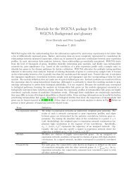
<strong>Weighted</strong> <strong>Gene</strong> <strong>Co</strong>-<strong>expression</strong> <strong>Network</strong> <strong>Analysis</strong><br />
(<strong>WGCNA</strong>)<br />
R Tutorial, Part B<br />
Module Eigengene, Survival time, and Proliferation<br />
Steve Horvath, Paul Mischel<br />
<strong>Co</strong>rrespondence: shorvath@mednet.ucla.edu, http://www.ph.ucla.edu/biostat/people/horvath.htm<br />
This is part B of a self-contained R software tutorial. The first few pages are very similar to those<br />
of part A, but here we focus on studying the brown module and relating individual genes to survival<br />
outcome. Thus, the reader will be able to reproduce all of our findings. This document also serves<br />
as a tutorial to weighted gene co-<strong>expression</strong> network analysis. Some familiarity with the R software<br />
is desirable but the document is fairly self-contained.<br />
This tutorial and the data files can be found at the following webpage:<br />
http://www.genetics.ucla.edu/labs/horvath/<strong>Co</strong><strong>expression</strong><strong>Network</strong>/ASPMgene<br />
More material on weighted network analysis can be found here<br />
http://www.genetics.ucla.edu/labs/horvath/<strong>Co</strong><strong>expression</strong><strong>Network</strong>/<br />
Abstract<br />
The data and biological implications are described in part A and in<br />
• Horvath S, Zhang B, Carlson M, Lu KV, Zhu S, Felciano RM, Laurance MF, Zhao W, Shu,<br />
Q, Lee Y, Scheck AC, Liau LM, Wu H, Geschwind DH, Febbo PG, Kornblum HI,<br />
Cloughesy TF, Nelson SF, Mischel PS (2006) <strong>Analysis</strong> of Oncogenic Signaling <strong>Network</strong>s in<br />
Glioblastoma Identifies ASPM as a Novel Molecular Target.<br />
Patient samples:<br />
Brain Cancer (GBM) microarray data involving the 3600 most connected genes. This file<br />
contains 2 sets: the first 55 arrays are the training set. The next 65 patients are the validation<br />
set. <strong>Co</strong>lumns corresponding to the 65 validation samples start with Set65<br />
Rows are genes, columns are patients. First 4 lines contain patient information (died=1), etc.<br />
<strong>Co</strong>ntents part B (the beginning overlaps with part A)<br />
*) <strong>Weighted</strong> brain cancer network construction based on *3600* most connected genes<br />
*) <strong>Gene</strong> significance and intramodular connectivity in data sets I and II<br />
*) Module Eigengene and its relationship to individual genes<br />
*) Regressing survival time on individual gene <strong>expression</strong> and the module eigengene<br />
1
# <strong>Gene</strong>ration of weighted gene co<strong>expression</strong> network:<br />
# Forms the topic of GBMtutorialPartAHorvath.doc which can be found at our webpage<br />
# Absolutely no warranty on the code. Please contact SH with suggestions.<br />
# CONTENTS<br />
# This document contains function for carrying out the following tasks<br />
# A) Assessing scale free topology and choosing the parameters of the adjacency function<br />
# using the scale free topology criterion (Zhang and Horvath 05)<br />
# B) <strong>Co</strong>mputing the topological overlap matrix<br />
# C) Defining gene modules using clustering procedures<br />
# D) Summing up modules by their first principal component (first eigengene)<br />
# E) Relating a measure of gene significance to the modules<br />
# F) Carrying out a within module analysis (computing intramodular connectivity)<br />
# and relating intramodular connectivity to gene significance.<br />
# Downloading the R software<br />
# 1) Go to http://www.R-project.org, download R and install it on your computer<br />
# After installing R, you need to install several additional R library packages:<br />
# For example to install Hmisc, open R,<br />
# go to menu "Packages\Install package(s) from CRAN",<br />
# then choose Hmisc. R will automatically install the package.<br />
# When asked "Delete downloaded files (y/N)? ", answer "y".<br />
# Do the same for some of the other libraries mentioned below. But note that<br />
# several libraries are already present in the software so there is no need to re-install them.<br />
# To get this tutorial and data files, go to the following webpage<br />
# http://www.genetics.ucla.edu/labs/horvath/<strong>Co</strong><strong>expression</strong><strong>Network</strong>/ASPMgene<br />
# Download the zip file containing:<br />
# 1) R function file: "<strong>Network</strong>Functions.txt", which contains several R functions<br />
# needed for <strong>Network</strong> <strong>Analysis</strong>.<br />
# 2) The data files and this tutorial<br />
# Unzip all the files into the same directory.<br />
# The user should copy and paste the following script into the R session.<br />
# Text after "#" is a comment and is automatically ignored by R.<br />
# Set the working directory of the R session by using the following command.<br />
# Please adapt the following path. Note that we use / instead of \ in the path.<br />
setwd("C:/Documents and Settings/shorvath/My<br />
Documents/ADAG/PaulMischel/GBMnetworkpaper/Webpage/BrainCancerTutorial")<br />
# read in the R libraries<br />
library(MASS) # standard, no need to install<br />
library(class) # standard, no need to install<br />
library(cluster)<br />
library(sma) # install it for the function plot.mat<br />
library(impute)# install it for imputing missing value<br />
library(Hmisc) # install it for the C-index calculations<br />
2
library(survival)<br />
# Memory<br />
# check the maximum memory that can be allocated<br />
memory.size(TRUE)/1024<br />
# increase the available memory<br />
memory.limit(size=4000)<br />
# Please adapt the following path to whereever the file <strong>Network</strong>Functions.txt<br />
# Please adapt the following path to whereever the file <strong>Network</strong>Functions.txt<br />
source(“C:/Documents and Settings/shorvath/My Documents/RFunctions/<strong>Network</strong>Functions.txt”)<br />
# the following contains <strong>expression</strong> data of the 3600 most connected genes (see part A)<br />
# across the 55 GBM sample data set and the 65 GBM sample set.<br />
dat0=read.csv("GBM3600Set55and65andClinicalInformation.csv")<br />
# the following data frame contains<br />
# the gene <strong>expression</strong> data: columns are genes, rows are arrays (samples)<br />
datExprdataOne =data.frame(t(dat0[-c(1:4),18:72]))<br />
datExprdataTwo=data.frame( t(dat0[-c(1:4),73:137]))<br />
names(datExprdataOne)=as.character( dat0$gbm133a[-c(1:4)])<br />
names(datExprdataTwo)=as.character( dat0$gbm133a[-c(1:4)])<br />
# these data frames contain the clinical data of the patients<br />
datClinicaldataOne=dat0[1:4,18:72]<br />
datClinicaldataTwo=dat0[1:4,73:137]<br />
datClinicaldataOne =data.frame(t(dat0[c(1:4),18:72]))<br />
names(datClinicaldataOne)=as.character(dat0[1:4,1])<br />
datClinicaldataTwo=data.frame( t(dat0[c(1:4),73:137]))<br />
names(datClinicaldataTwo)=as.character(dat0[1:4,1])<br />
# for (i in c(1:dim(datExprdataOne)[[1]]) ) {datExprdataOne[i,]=as.numeric(datExprdataOne[i,])}<br />
# for (i in c(1:dim(datExprdataTwo)[[1]]) ) {datExprdataTwo[i,]=as.numeric(datExprdataTwo[i,])}<br />
# this data frame contains information on the probesets<br />
datSummary=dat0[-c(1:4),c(1:17)]<br />
dim(datExprdataOne)<br />
dim(datExprdataTwo)<br />
dim(datSummary)<br />
rm(dat0);collect_garbage()<br />
Quotes from an unrecognized statistician:<br />
"What is best let alone, that accursed thing is not always what least allures."<br />
"Aye, aye! and I'll chase him round Good Hope, and round the Horn, and round the Norway Maelstrom, and round<br />
perdition's flames before I give him up."<br />
“...to the last I grapple with thee; from hell's heart I stab at thee; for hates sake I spit my last breath at thee.”<br />
Captain Ahab in “Moby Dick” by Melville<br />
3
#SOFT THRESHOLDING<br />
#As described in tutorial A, we use the following power for the power adjacency function.<br />
beta1=6<br />
DegreedataOne=Soft<strong>Co</strong>nnectivity(datExprdataOne,power=beta1)-1<br />
DegreedataTwo= Soft<strong>Co</strong>nnectivity(datExprdataTwo,power=beta1)-1<br />
# Let’s create a scale free topology plot for the dataOne and dataTwo network<br />
par(mfrow=c(2,2))<br />
ScaleFreePlot1(DegreedataOne, AF1=paste("data set I, power=",beta1), truncated1=F);<br />
ScaleFreePlot1(DegreedataTwo, AF1=paste("data set II, power=",beta1), truncated1=F);<br />
# this relates the whole network connectivity measures in the 2 networks<br />
scatterplot1(DegreedataOne, DegreedataTwo,xlab1="3600 genes, connectivity in data I",ylab1="k<br />
in data II",title1="k (data I) vs k (data II)",cex1=1)<br />
# In contrast to the plot in tutorial part A which involves 8000 genes,<br />
# these plots are for the network comprised of 3600 genes<br />
4
# Module Detection (detailed in part A!)<br />
# To group genes with coherent <strong>expression</strong> profiles into modules, we use average linkage<br />
# hierarchical clustering, which uses the topological overlap measure as dissimilarity.<br />
# This code allows one to restrict the analysis to the most connected genes,<br />
# which may speed up calculations when it comes to module detection.<br />
DegCut = 3601 # number of most connected genes that will be considered<br />
DegreeRank = rank(-DegreedataOne)<br />
vardataOne=as.vector(apply(datExprdataOne,2,var))<br />
vardataTwo= as.vector(apply(datExprdataTwo,2,var))<br />
# Since we want to compare the results between data sets I and II we restrict the analysis to<br />
# the most connected probesets with non-zero variance in both data sets<br />
restDegree = DegreeRank 0 &vardataTwo>0<br />
# The following code computes the topological overlap matrix<br />
dissGTOMdataOne=TOMdist1(abs(cor(datExprdataOne[,restDegree],use="p"))^beta1)<br />
collect_garbage()<br />
hierGTOMdataOne = hclust(as.dist(dissGTOMdataOne),method="average");<br />
collect_garbage()<br />
par(mfrow=c(1,1))<br />
plot(hierGTOMdataOne,labels=F,main="Dendrogram, data set I")<br />
5
# By our definition, modules correspond to branches of the tree.<br />
# The function modulecolor2 colors each gene by the branches that<br />
# result from choosing a particular height cut-off.<br />
# GREY IS RESERVED to color genes that are not part of any module.<br />
# We only consider modules that contain at least 125 genes.<br />
# But in other applications smaller modules may also be of interest.<br />
colorhdataOne=as.character(modulecolor2(hierGTOMdataOne,h1=.94, minsize1=125))<br />
par(mfrow=c(2,1))<br />
plot(hierGTOMdataOne, main="data set I", labels=F, xlab="", sub="");<br />
hclustplot1(hierGTOMdataOne,colorhdataOne, title1="Module membership: data I")<br />
# COMMENT: The colors are assigned based on module size. Turquoise (others refer to it as cyan)<br />
# colors the largest module, next comes blue, etc. Just type table(colorhdataOne) to figure out<br />
# which color corresponds to what module size.<br />
# This is Figure 1a in our article<br />
Quote: Two archetypes have defined America’s sense of destiny. One is the self-made man, who<br />
believes he will get rich through his own hard work. The other is the gambler, who believes that with the<br />
the next turn of the cards, providence will deliver the Main Chance. Jackson Lears “Something for<br />
Nothing: luck in America”.<br />
6
# NOW WE DEFINE THE GENE SIGNIFICANCE VARIABLE,<br />
# which equals minus log10 of the univarite <strong>Co</strong>x regression p-value for predicting survival<br />
# on the basis of the gene epxression info<br />
# Here we define the prognostic gene significance measures in the data set I and data set II<br />
GSdataOne=-log10(datSummary$Set55<strong>Co</strong>xpvalue)[restDegree]<br />
GSdataTwo=-log10(datSummary$Set65<strong>Co</strong>xpvalue)[restDegree]<br />
# The following produces heatmap plots for each module.<br />
# Here the rows are genes and the columns are samples.<br />
# Well defined modules results in characteristic band structures since the corresponding genes are<br />
# highly correlated.<br />
par(mfrow=c(1,1), mar=c(1, 2, 4, 1))<br />
which.module="brown"<br />
ClusterSamples=hclust(dist(datExprdataOne[,restDegree][,colorhdataOne==which.module]<br />
),method="average")<br />
# for this module we find<br />
plot.mat(t(scale(datExprdataOne[ClusterSamples$order,restDegree][,colorhdataOne==which.modu<br />
le ]) ),nrgcols=30,rlabels=T, clabels=T,rcols=which.module,<br />
title=paste("dataOne set, heatmap",which.module,"module") )<br />
7
# Now we extend the color definition to all genes by coloring all non-module<br />
# genes grey.<br />
color1=rep("grey",dim(datExprdataOne)[[2]])<br />
color1[restDegree]=as.character(colorhdataOne)<br />
# The function DegreeInOut computes the whole network connectivity kTotal,<br />
# the within module connectivity (kWithin). kOut=kTotal-kWithin and<br />
# and kDiff=kIn-kOut=2*kIN-kTotal<br />
AlldegreesdataOne=DegreeInOut(abs(cor(datExprdataOne[,restDegree],use="p"))^beta1,colorhdat<br />
aOne)<br />
names(AlldegreesdataOne)<br />
[1] "kTotal" "kWithin" "kOut" "kDiff"<br />
# The function WithinModule<strong>Analysis</strong>1 relates the connectivities kTotal, kWithin etc to the gene<br />
# gene significance information within each module.<br />
# Output: first column reports the p-value of the Spearman correlation<br />
# test between the connectivity measure and the node significance (gene significance).<br />
# The second column contains the Spearman correlation between connectivity<br />
# and node significance. The remaining columns list Spearman correlations.<br />
WithinModule<strong>Analysis</strong>1(AlldegreesdataOne,GSdataOne,colorhdataOne)<br />
Excerpt<br />
couleur: brown<br />
variable NS.<strong>Co</strong>rPval NS.cor kTotal kWithin kOut kDiff<br />
kTotal kTotal 1.9e-08 0.40 1.00 0.910 0.420 0.59<br />
kWithin kWithin 7.1e-19 0.59 0.91 1.000 0.074 0.86<br />
kOut kOut 7.0e-06 -0.32 0.42 0.074 1.000 -0.38<br />
kDiff kDiff 1.1e-25 0.67 0.59 0.860 -0.380 1.00<br />
# <strong>Co</strong>mments: Warning messages can be ignored at this point, they simply point out<br />
# that the Spearman test p-values may be incorrect due to ties in: cor.test (Spearman correlation)<br />
# The prefix "NS" means node significance (here gene significance).<br />
# For the brown module we find that kWithin is significantly correlated with<br />
# gene signficance (p=7.1e-19, corresonding Spearman correlation= 0.59)<br />
# Note that kWithin and kTotal are highly correlated (Spearman correlation=0.91).<br />
8
# The following plots show the gene significance vs intramodular connectivity<br />
# in the data set I<br />
colorlevels=levels(factor(colorhdataOne))<br />
par(mfrow=c(2,3))<br />
for (i in c(1:length(colorlevels) ) ) {<br />
whichmodule=colorlevels[[i]];restrict1=colorhdataOne==whichmodule<br />
scatterplot1(AlldegreesdataOne$kWithin[restrict1],<br />
GSdataOne[restrict1],col1=colorhdataOne[restrict1],xlab1="<strong>Co</strong>nnectivity k, GBM set<br />
1",ylab1="Survival Association, -log(p)",title1= paste("set I,", whichmodule))<br />
}<br />
# If you don’t see a relationship betwen GS and connectivity in your data,<br />
# and, more importantly, if the following is not significant<br />
# ModuleEnrichment1(GSdataOne,colorhdataOne)<br />
# then check whether you read in the data correctly. Here is quote from an unrecognized statistician #who accidentally<br />
permuted the relationship between datExpr and GS.<br />
# Quote:<br />
#"I cudda had class! I cudda been a contender! I cudda been somebody, instead of a bum which is<br />
what I am." Marlon Brando, On the Waterfront<br />
9
# Now we repeat the within module analysis in data set II<br />
AlldegreesdataTwo=DegreeInOut(abs(cor(datExprdataTwo[,restDegree],use="p"))^beta1,colorhdat<br />
aOne)<br />
WithinModule<strong>Analysis</strong>1(AlldegreesdataTwo,GSdataTwo,colorhdataOne)<br />
#Excerpt<br />
couleur: brown<br />
variable NS.<strong>Co</strong>rPval NS.cor kTotal kWithin kOut kDiff<br />
kTotal kTotal 5.2e-12 0.480 1.00 0.85 0.60 0.49<br />
kWithin kWithin 6.5e-19 0.590 0.85 1.00 0.20 0.84<br />
kOut kOut 6.6e-01 0.032 0.60 0.20 1.00 -0.32<br />
kDiff kDiff 3.9e-17 0.570 0.49 0.84 -0.32 1.00<br />
# The following plots show the gene significance vs intramodular connectivity<br />
# in the data set II<br />
colorlevels=levels(factor(colorhdataOne))<br />
par(mfrow=c(2,3))<br />
for (i in c(1:length(colorlevels) ) ) {<br />
whichmodule=colorlevels[[i]];restrict1=colorhdataOne==whichmodule<br />
scatterplot1(AlldegreesdataTwo$kWithin[restrict1],<br />
GSdataTwo[restrict1],col1=colorhdataOne[restrict1],xlab1="<strong>Co</strong>nnectivity k, GBM set<br />
II",ylab1="Survival Association, -log(p)",title1= paste("set II,", whichmodule))<br />
}<br />
10
# Now we create Figure 2 a and b) in the manuscript<br />
par(mfrow=c(1,2))<br />
whichmodule="brown";restrict1=colorhdataOne==whichmodule<br />
scatterplot1(AlldegreesdataOne$kWithin[restrict1], GSdataOne[restrict1],<br />
col1=colorhdataOne[restrict1],xlab1="<strong>Co</strong>nnectivity (k) - GBM set 1",ylab1="Survival Association:<br />
–log10(p)",title1="")<br />
scatterplot1(AlldegreesdataTwo$kWithin[restrict1], GSdataTwo[restrict1],<br />
col1=colorhdataOne[restrict1],xlab1="<strong>Co</strong>nnectivity (k) - GBM set 2",ylab1="Survival<br />
Association: –log10(p)",title1="")<br />
cor= 0.59 p= 7.1e-19<br />
cor= 0.59 p= 6.5e-19<br />
Survival Association: -log10(p)<br />
0.0 0.5 1.0 1.5 2.0 2.5<br />
Survival Association: -log10(p)<br />
0.0 0.5 1.0 1.5 2.0 2.5 3.0 3.5<br />
10 20 30 40 50<br />
<strong>Co</strong>nnectivity (k) - GBM set 1<br />
0 5 10 15 20 25<br />
<strong>Co</strong>nnectivity (k) - GBM set 2<br />
11
# Now we relate the connectivities between set I and II<br />
whichmodule="brown";restrict1=colorhdataOne==whichmodule<br />
scatterplot1(AlldegreesdataOne$kWithin[restrict1], AlldegreesdataTwo$kWithin[restrict1],<br />
col1=colorhdataOne[restrict1],xlab1="<strong>Co</strong>nnectivity k, GBM set I",ylab1="<strong>Co</strong>nnectivity k, GBM<br />
set II",title1="")<br />
cor= 0.79 p=
# Module Eigengenes<br />
# This code yields the module eigengene for each module<br />
PCdataOne=ModulePrin<strong>Co</strong>mps1(datExprdataOne[,restDegree],colorhdataOne)[[1]]<br />
PCdataTwo=ModulePrin<strong>Co</strong>mps1(datExprdataTwo[,restDegree],colorhdataOne)[[1]]<br />
# Here we combine data sets I and II to arrive at a combined module eigengene<br />
PC<strong>Co</strong>mbined=ModulePrin<strong>Co</strong>mps1(rbind(datExprdataOne[,restDegree],datExprdataTwo[,restDegre<br />
e]),colorhdataOne)[[1]]<br />
# The following defines the module eigengene of the brown module<br />
PCbrowndataOne=PCdataOne$PCbrown<br />
PCbrowndataTwo=PCdataTwo$PCbrown<br />
PCbrown<strong>Co</strong>mbined=PC<strong>Co</strong>mbined$PCbrown<br />
#The following output<br />
datSummary$<strong>Gene</strong>.Symbol[restDegree][colorhdataOne=="brown"]<br />
# the following lists the 10 most connected genes in the brown module.<br />
topNumberHubs=10<br />
datframe=data.frame(<strong>Gene</strong>Symbol=datSummary$<strong>Gene</strong>.Symbol[restDegree],AlldegreesdataOne)[c<br />
olorhdataOne=="brown",]<br />
datframe[rank(-datframe$kWithin)
# The following vectors contain the gene expresson profiles of the top 10 hub genes<br />
TOP2AdataOne= datExprdataOne[,datSummary$<strong>Gene</strong>.Symbol=="TOP2A"]<br />
TOP2AdataTwo= datExprdataTwo[,datSummary$<strong>Gene</strong>.Symbol=="TOP2A"]<br />
TOP2A<strong>Co</strong>mbined=c(TOP2AdataOne, TOP2AdataTwo)<br />
RACGAP1dataOne= datExprdataOne[,datSummary$<strong>Gene</strong>.Symbol=="RACGAP1"]<br />
RACGAP1dataTwo= datExprdataTwo[,datSummary$<strong>Gene</strong>.Symbol=="RACGAP1"]<br />
RACGAP1<strong>Co</strong>mbined=c(RACGAP1dataOne, RACGAP1dataTwo)<br />
KIF4AdataOne= datExprdataOne[,datSummary$<strong>Gene</strong>.Symbol=="KIF4A"]<br />
KIF4AdataTwo= datExprdataTwo[,datSummary$<strong>Gene</strong>.Symbol=="KIF4A"]<br />
KIF4A<strong>Co</strong>mbined=c(KIF4AdataOne, KIF4AdataTwo)<br />
TPX2dataOne= datExprdataOne[,datSummary$<strong>Gene</strong>.Symbol=="TPX2"]<br />
TPX2dataTwo= datExprdataTwo[,datSummary$<strong>Gene</strong>.Symbol=="TPX2"]<br />
TPX2<strong>Co</strong>mbined=c(TPX2dataOne, TPX2dataTwo)<br />
CDC2dataOne= datExprdataOne[,datSummary$<strong>Gene</strong>.Symbol=="CDC2"]<br />
CDC2dataTwo= datExprdataTwo[,datSummary$<strong>Gene</strong>.Symbol=="CDC2"]<br />
CDC2<strong>Co</strong>mbined=c(CDC2dataOne, CDC2dataTwo)<br />
EZH2dataOne= datExprdataOne[,datSummary$<strong>Gene</strong>.Symbol=="EZH2"]<br />
EZH2dataTwo= datExprdataTwo[,datSummary$<strong>Gene</strong>.Symbol=="EZH2"]<br />
EZH2<strong>Co</strong>mbined=c(EZH2dataOne, EZH2dataTwo)<br />
CDC20dataOne= datExprdataOne[,datSummary$<strong>Gene</strong>.Symbol=="CDC20"]<br />
CDC20dataTwo= datExprdataTwo[,datSummary$<strong>Gene</strong>.Symbol=="CDC20"]<br />
CDC20<strong>Co</strong>mbined=c(CDC20dataOne, CDC20dataTwo)<br />
KIF14dataOne= datExprdataOne[,datSummary$<strong>Gene</strong>.Symbol=="KIF14"]<br />
KIF14dataTwo= datExprdataTwo[,datSummary$<strong>Gene</strong>.Symbol=="KIF14"]<br />
KIF14<strong>Co</strong>mbined=c(KIF14dataOne, KIF14dataTwo)<br />
RAMPdataOne= datExprdataOne[,datSummary$<strong>Gene</strong>.Symbol=="RAMP"]<br />
RAMPdataTwo= datExprdataTwo[,datSummary$<strong>Gene</strong>.Symbol=="RAMP"]<br />
RAMP<strong>Co</strong>mbined=c(RAMPdataOne, RAMPdataTwo)<br />
ASPMdataOne= datExprdataOne[,datSummary$<strong>Gene</strong>.Symbol=="ASPM"]<br />
ASPMdataTwo= datExprdataTwo[,datSummary$<strong>Gene</strong>.Symbol=="ASPM"]<br />
ASPM<strong>Co</strong>mbined=c(ASPMdataOne, ASPMdataTwo)<br />
# To get the connectivity of Ki67 use the following code<br />
AlldegreesdataOne[datSummary$<strong>Gene</strong>.Symbol[restDegree]=="MKI67",]<br />
kTotal kWithin kOut kDiff<br />
212022_s_at 23.44682 13.76298 9.68384 4.079146<br />
#The following genes are standard markers of proliferation<br />
PCNAdataOne= datExprdataOne[,datSummary$<strong>Gene</strong>.Symbol=="PCNA"]<br />
PCNAdataTwo= datExprdataTwo[,datSummary$<strong>Gene</strong>.Symbol=="PCNA"]<br />
PCNA<strong>Co</strong>mbined=c(PCNAdataOne,PCNAdataTwo)<br />
MKI67dataOne= datExprdataOne[,datSummary$<strong>Gene</strong>.Symbol=="MKI67"]<br />
MKI67dataTwo= datExprdataTwo[,datSummary$<strong>Gene</strong>.Symbol=="MKI67"]<br />
MKI67<strong>Co</strong>mbined=c(MKI67dataOne,MKI67dataTwo)<br />
14
#Now we relate the module eigengene to proliferation markers PCNA, KI67 and ASPM<br />
par(mfrow=c(3,2))<br />
scatterplot1(MKI67dataOne,PCbrowndataOne,xlab1="Ki67, data 1",ylab1="Module Eigengene",<br />
title1="data 1: 55 samples")<br />
scatterplot1(MKI67dataTwo,PCbrowndataTwo ,xlab1="Ki67, data 1I",ylab1="Module Eigengene",<br />
title1="data 2: 65 samples")<br />
scatterplot1(PCNAdataOne,PCbrowndataOne,xlab1="PCNA, data 1",ylab1="Module Eigengene",<br />
title1="data 1: 55 samples ")<br />
scatterplot1(PCNAdataTwo,PCbrowndataTwo ,xlab1="PCNA, data 2",ylab1="Module<br />
Eigengene", title1="data 2: 65 samples")<br />
scatterplot1(ASPMdataOne,PCbrowndataOne,xlab1="ASPM, data 1",ylab1="Module Eigengene",<br />
title1="data 1: 55 samples")<br />
scatterplot1(ASPMdataTwo,PCbrowndataTwo ,xlab1="ASPM, data 2",ylab1="Module<br />
Eigengene", title1="data 2: 65 samples")<br />
Module Eigengene<br />
-0.2 0.1 0.4<br />
data 1: 55 samples cor= 0.63 p= 5.2e-07<br />
100 200 300 400 500 600<br />
Ki67, data 1<br />
data 1: 55 samples cor= 0.84 p=
# Now we relate the marker <strong>expression</strong> and the module eigengene to the survival outcome in GBM<br />
timedataOne=datClinicaldataOne$SurvivalTimeDays<br />
dieddataOne=datClinicaldataOne$died<br />
timedataTwo=datClinicaldataTwo$SurvivalTimeDays<br />
dieddataTwo=datClinicaldataTwo$died<br />
time<strong>Co</strong>mbined=c(timedataOne,timedataTwo)<br />
died<strong>Co</strong>mbined= c(dieddataOne,dieddataTwo)<br />
# here we regress survival time on the module eigengene<br />
summary(coxph(Surv(time<strong>Co</strong>mbined,died<strong>Co</strong>mbined)~PCbrown<strong>Co</strong>mbined))$waldtest<br />
test df pvalue<br />
6.37000000 1.00000000 0.01161113<br />
#here we regress survival time on the top 10 hub genes<br />
summary(coxph(Surv(time<strong>Co</strong>mbined,died<strong>Co</strong>mbined)~TOP2A<strong>Co</strong>mbined))$waldtest<br />
test df pvalue<br />
1.107000e+01 1.000000e+00 8.789649e-04<br />
summary(coxph(Surv(time<strong>Co</strong>mbined,died<strong>Co</strong>mbined)~RACGAP1<strong>Co</strong>mbined))$waldtest<br />
test df pvalue<br />
9.340000000 1.000000000 0.002247980<br />
summary(coxph(Surv(time<strong>Co</strong>mbined,died<strong>Co</strong>mbined)~KIF4A<strong>Co</strong>mbined))$waldtest<br />
test df pvalue<br />
8.780000000 1.000000000 0.003043759<br />
summary(coxph(Surv(time<strong>Co</strong>mbined,died<strong>Co</strong>mbined)~TPX2<strong>Co</strong>mbined))$waldtest<br />
test df pvalue<br />
9.430000000 1.000000000 0.002136835<br />
summary(coxph(Surv(time<strong>Co</strong>mbined,died<strong>Co</strong>mbined)~CDC2<strong>Co</strong>mbined))$waldtest<br />
test df pvalue<br />
7.210000000 1.000000000 0.007233725<br />
summary(coxph(Surv(time<strong>Co</strong>mbined,died<strong>Co</strong>mbined)~EZH2<strong>Co</strong>mbined))$waldtest<br />
test df pvalue<br />
5.12000000 1.00000000 0.02369322<br />
summary(coxph(Surv(time<strong>Co</strong>mbined,died<strong>Co</strong>mbined)~CDC20<strong>Co</strong>mbined))$waldtest<br />
test df pvalue<br />
8.860000000 1.000000000 0.002916241<br />
summary(coxph(Surv(time<strong>Co</strong>mbined,died<strong>Co</strong>mbined)~KIF14<strong>Co</strong>mbined))$waldtest<br />
test df pvalue<br />
9.550000000 1.000000000 0.002003858<br />
summary(coxph(Surv(time<strong>Co</strong>mbined,died<strong>Co</strong>mbined)~RAMP<strong>Co</strong>mbined))$waldtest<br />
test df pvalue<br />
5.94000000 1.00000000 0.01480329<br />
summary(coxph(Surv(time<strong>Co</strong>mbined,died<strong>Co</strong>mbined)~ASPM<strong>Co</strong>mbined))$waldtest<br />
test df pvalue<br />
16
7.580000000 1.000000000 0.005889949<br />
# here we regress survival time on the proliferation markers<br />
summary(coxph(Surv(time<strong>Co</strong>mbined,died<strong>Co</strong>mbined)~PCNA<strong>Co</strong>mbined))$waldtest<br />
test df pvalue<br />
5.36000000 1.00000000 0.02055703<br />
summary(coxph(Surv(time<strong>Co</strong>mbined,died<strong>Co</strong>mbined)~MKI67<strong>Co</strong>mbined))$waldtest<br />
test df pvalue<br />
2.2800000 1.0000000 0.1309132<br />
# Here is some code for exporting a summary of the data<br />
datout=data.frame(datSummary[restDegree,], colorhdataOne,GSdataOne, AlldegreesdataOne,<br />
GSdataTwo, AlldegreesdataTwo)<br />
write.table(datout, "datSummaryRestDegree.csv", sep=",",row.names=F)<br />
Quote<br />
I thought the following four rules would be enough, provided that I made a firm and constant resolution not to<br />
fail even once in the observance of them. The first was never to accept anything as true if I had not evident<br />
knowledge of its being so; that is, carefully to avoid precipitancy and prejudice, and to embrace in my<br />
judgment only what presented itself to my mind so clearly and distinctly that I had no occasion to doubt it.<br />
The second, to divide each problem I examined into as many parts as was feasible, and as was requisite for<br />
its better solution. The third, to direct my thoughts in an orderly way; beginning with the simplest objects,<br />
those most apt to be known, and ascending little by little, in steps as it were, to the knowledge of the most<br />
complex; and establishing an order in thought even when the objects had no natural priority one to another.<br />
And the last, to make throughout such complete enumerations and such general surveys that I might be<br />
sure of leaving nothing out. These long chains of perfectly simple and easy reasonings by means of which<br />
geometers are accustomed to carry out their most difficult demonstrations had led me to fancy that<br />
everything that can fall under human knowledge forms a similar sequence; and that so long as we avoid<br />
accepting as true what is not so, and always preserve the right order of deduction of one thing from another,<br />
there can be nothing too remote to be reached in the end, or to well hidden to be discovered.<br />
Discours de la Méthode. 1637. Descartes, René (1596-1650)<br />
# THE END<br />
17