Cruise Report - jamstec japan agency for marine-earth science and ...
Cruise Report - jamstec japan agency for marine-earth science and ...
Cruise Report - jamstec japan agency for marine-earth science and ...

You also want an ePaper? Increase the reach of your titles
YUMPU automatically turns print PDFs into web optimized ePapers that Google loves.
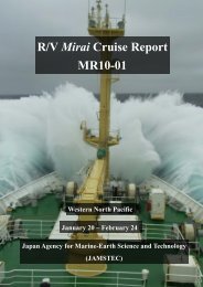
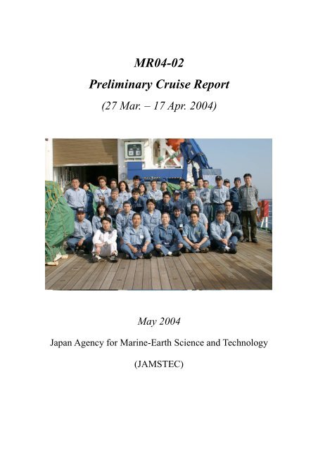
MR04-02<br />
Preliminary <strong>Cruise</strong> <strong>Report</strong><br />
(27 Mar. – 17 Apr. 2004)<br />
May 2004<br />
Japan Agency <strong>for</strong> Marine-Earth Science <strong>and</strong> Technology<br />
(JAMSTEC)
Preface<br />
Mutsu Institute <strong>for</strong> Oceanography (MIO) has conducted time-series observational<br />
study <strong>for</strong> biogeochemistry in the northwestern North Pacific with mooring systems. However<br />
seasonal variability in biogeochemistry <strong>and</strong> physical oceanography can not be clarified precisely<br />
without traditional repeatable observation by research vessel. It is no doubt that data in winter<br />
season are absolutely poor compared with those in other seasons. There<strong>for</strong>e main purpose of<br />
this cruise was to obtain oceanographic data in the late winter <strong>and</strong>/or the early spring.<br />
However rough sea toyed us heavily as we expected. We should wait a chance <strong>for</strong><br />
observation or gave up observation at some stations. Nevertheless valuable data could be<br />
obtained during this cruise. For instance, it was certified that surface mixed layer was still<br />
thick <strong>and</strong> extinction rate of light intensity in the water column was small, which is indicative of<br />
that amount of suspended matter including living plankton was still a little.<br />
As described above, we were in trouble <strong>for</strong> bad weather <strong>and</strong> problem on wire cable<br />
<strong>and</strong> instrument. Thanks to captain Akamine <strong>and</strong> ship crew, <strong>and</strong> support stuff from Marine<br />
Works Japan <strong>and</strong> Global Ocean Development, main mission was completed successfully.<br />
Especially, Mr. Kita, a new chief officer, did work so hard <strong>and</strong> devotedly. Owing to his<br />
appropriate leadership, every deck work was done smoothly <strong>and</strong> safely. We would like to<br />
welcome him to MIRAI.<br />
As <strong>for</strong> MIO, this cruise was the first cruise since the last year’s cruise we lost<br />
mooring system. The scientific cruise without mooring work was not challenging enough. I<br />
wish that I will bring our mooring system on board <strong>and</strong> restart time-series observation with<br />
mooring system the next time.<br />
April 16, 2004<br />
Makio Honda<br />
Principal Investigator of MR04-02
Contents<br />
1.Outline of MR04-02<br />
1.1 <strong>Cruise</strong> summary 1<br />
1.2 Track <strong>and</strong> log 3<br />
1.3 List of participants 5<br />
2. General observation<br />
2.1 Meteorological observations 6<br />
2.2 Physical oceanographic observation<br />
2.2.1 CTD casts <strong>and</strong> water sampling 13<br />
2.2.2 Salinity measurement 32<br />
2.2.3 Shipboard ADCP observation 34<br />
2.3 Sea surface monitoring 37<br />
2.4Dissolved oxygen 40<br />
2.5 Nutrients 46<br />
2.6 Total dissolved Inorganic carbon-TDIC-<br />
2.6.1 water column TDIC 48<br />
2.6.2 Sea surface TDIC 51<br />
2.7 Total alkalinity 53<br />
2.8 Chl-a 56<br />
3. Special observation<br />
3.1 Vertical distribution of suspended particles 58<br />
3.2 Optical measurement 59<br />
3.3 Primary productivity 65<br />
3.4 Th-234 <strong>and</strong> export flux 68<br />
3.5 Horizontal distribution of suspended particles 69<br />
3.6 Horizontal distribution of planktonic <strong>for</strong>aminifera 71<br />
3.6 Aeolion dust <strong>and</strong> Ba 73<br />
3.7 Trace elements 76<br />
3.8 Remote Access Sampler sample 77<br />
4. Geological observation<br />
4.1 Swath bathymetry 85<br />
4.2 Sea surface gravity 87<br />
4.3 Sea surface three-component magnetic field 88<br />
5. Remotely sensing observation 89<br />
Appendix<br />
CTD/CMS bottle list <strong>and</strong> routine data 94
1.Outline of MR04-02<br />
1.1 <strong>Cruise</strong> summary<br />
Makio HONDA (JAMSTEC MIO)<br />
We planned to visit 8 stations <strong>and</strong> conducted various observations such as hydrocast, in-situ<br />
pumping <strong>and</strong> water column optical measurement. The first station planned was station 1 (K1: timeseries<br />
observation <strong>for</strong> our biogeochemical study <strong>and</strong> one of principal stations). However weather <strong>and</strong><br />
sea condition did not enable us to do so. We started our observation from station 8<br />
Station 8<br />
When the first hydrocast was conducted, “kink of wire cable” phenomena took place because of rough<br />
sea. Thanks to Marine Works’ technicians <strong>and</strong> MIRAI’s waisters, cable was repaired <strong>and</strong> hydrocast<br />
work could be re-started <strong>and</strong>, as a result, three hydrocasts were conducted at this station. This station<br />
was close to Hokkaido Isl<strong>and</strong> (300 miles off Kushiro) <strong>and</strong>, there<strong>for</strong>e, samples which were expected to<br />
have l<strong>and</strong> characteristics could be obtained.<br />
Based on the weather condition, we decided to visit station 5 (K3) which is one of our timeseries<br />
observation point.<br />
Station 5 (K3)<br />
We planned three hydrocasts <strong>and</strong> two in-situ pumpings. However the sea condition was getting worse<br />
<strong>and</strong> worse when we deployed CTD/CMS <strong>for</strong> routine cast, <strong>and</strong> we could not but suspend hydrocasts <strong>and</strong><br />
other observations. As a result, only CTD profile by 1000 m <strong>and</strong> water upper 300 m (<strong>for</strong> radio nuclide<br />
<strong>and</strong> trace elements) <strong>and</strong> water from five layer upper 100 m <strong>for</strong> “routine” (basic elements such as salinity,<br />
nutrients <strong>and</strong> carbonate chemistry) were obtained. A good thing was that optical measurement could be<br />
conducted be<strong>for</strong>e leaving this station.<br />
Although we planned to go northward on 160 degree-E meridian line, strong west wind permitted us to<br />
do so, <strong>and</strong> we moved toward station 1 (K1).<br />
Station 1 (K1):<br />
Fortunately weather <strong>and</strong> sea condition were not so bad <strong>and</strong> all menu (three hydrocasts, three in-situ<br />
pumpings optical measurements, <strong>and</strong> incubation of primary productivity) were successfully completed.<br />
Air temperature was about 1 degree-C <strong>and</strong> surface water temperature was about 2 degree-C. We had a<br />
little snow at this station. Marine works’ technicians were freezing during water distribution. Sea<br />
condition was still good <strong>and</strong> we could sequentially conducted observations at station 2 (K2) <strong>and</strong> station 6<br />
(KNOT).<br />
Station 2 (K2):<br />
As wind was stronger at this station than station K1, we felt colder. Water temperature was about 1<br />
degree-C <strong>and</strong> lower than that at station 1. Two hydrocasts, <strong>and</strong> two in-situ pumpings, optical<br />
measurements, <strong>and</strong> incubation of primary productivity were completed. Surface mixed layer defined<br />
with 0.125 criteria of sigma-theta was still 130 m <strong>and</strong> this area is still in winter mode. However we felt<br />
that spring has come soon.<br />
Station6 (KNOT):<br />
This station is the <strong>for</strong>mer Japanese time-series observation station under umbrella of JGOFS North<br />
Pacific Process Study. Some cooperative Japanese scientists including our group try to keep timer-series<br />
1
observation. Two hydrocasts, <strong>and</strong> two in-situ pumpings, optical measurements, <strong>and</strong> incubation of<br />
primary productivity were completed.<br />
Last four days were the busiest days on this cruise <strong>and</strong> most of participants suffered from lack of sleep.<br />
The rest of time <strong>for</strong> observation was limited. It seemed that observation at only one station<br />
was possible. We decided to go to station 3 (K2.5) <strong>and</strong> go southward to station 5 (35N, 160E) along<br />
160E meridian line without waiting chance <strong>for</strong> observation if sea condition was not friendly. After all,<br />
we skipped full <strong>and</strong> rest of observation at station 3(K2.5) <strong>and</strong> 4(K3), respectively. However underway<br />
observation such as measurements of water temperature, salinity, chlorophyll, <strong>and</strong> collection of<br />
suspended particles could be done along 160E line from 43N to 35N.<br />
Station 5 (35N)<br />
Meteorological <strong>and</strong> oceanographic condition was largely different from those at northern stations (north<br />
40N). Air temperature <strong>and</strong> water temperature were approximately 17 degree-C. We could work on<br />
deck with half-sleeves shirts. We conducted two hydrocasts, two in-situ pumping <strong>and</strong> optical<br />
measurement. These data will be useful <strong>and</strong> helpful as reference data against that from northern stations.<br />
After observation at station 5, we discussed more observation at station 4 (K3). However<br />
weather report showing horizontal distribution of atmospheric low pressure was pessimistic <strong>for</strong><br />
observation <strong>and</strong> time of our cruise was almost out. There<strong>for</strong>e we decided to finish our observation<br />
during this cruise <strong>and</strong> made our direction toward Shimonoseki.<br />
2
1.2 Track <strong>and</strong> log<br />
3
U.T.C. S.M.T. Position<br />
Date Time Date Time Lat. Lon.<br />
3/27 00:00 3/26 09:00 35-27.13N 139-38.84E Departure of Yokohama<br />
3/29 20:42 3/30 05:42 41-30N 145-30E Arrival at Station No.8<br />
3/30 00:29 3/30 09:29 41-29.96N 145-48.07E CTD-01 cast (300m)<br />
07:32 16:32 41-29.92N 145-48.38E CTD-test cast (300m)<br />
08:41 17:41 41-30.05N 145-48.96E CTD-02 cast (5,500m)<br />
14:00 23:00 - - Departure of Station No.8<br />
4/1 19:00 4/2 04:00 39-00N 160-00E Arrival at Station No.4 (K3)<br />
19:19 04:19 39-04N 160-00E Calibration <strong>for</strong> magnetometer<br />
4/2 08:55 17:55 39-00.06N 160-00.09E CTD-03 cast (300m)<br />
4/3 00:40 4/3 09:40 39-00.11N 160-00.43E Underwater optical measurement (Free fall) #01<br />
01:27 10:27 39-00.18N 160-00.48E CTD-04 cast (1,000m)<br />
02:30 11:30 - - Departure of Station No.4<br />
4/5 19:30 4/6 04:30 51-00N 165-00E Arrival at Station No.1 (K1)<br />
20:17 05:17 50-59.95N 165-00.07E In situ pumping (LVP) #01 (200m, 1 hour)<br />
22:55 07:55 50-59.98N 165-00.26E CTD-05 cast (300m)<br />
23:53 08:53 50-59.74N 164-59.86E LVP #02 (200m, 1 hour)<br />
4/6 02:13 4/6 11:13 51-00.05N 165-00.49E Free fall #02<br />
02:38 11:38 51-00.10N 165-00.29E CTD-06 cast (3,000m)<br />
05:45 14:45 51-00.47N 164-59.19E LVP #03 (200m, 6 hours)<br />
12:20 21:20 50-59.99N 164-59.93E CTD-07 cast (51m)<br />
12:42 21:42 - - Departure of Station No.1<br />
4/7 02:27 4/7 11:27 48-20.27N 161-30.74E Free fall-03 cast<br />
4/7 10:00 4/7 19:00 47-00N 160-00E Arrival at Station No.2 (K2)<br />
10:08 19:08 47-00.28N 160-00.11E LVP #04 (200m, 1 hour)<br />
12:37 21:37 47-00.01N 160-00.25E CTD-08 cast (3,000m)<br />
15:48 4/8 00:48 47-00.07N 160-01.91E LVP #05 (200m, 1 hour)<br />
18:18 03:18 47-00.03N 159-59.90E CTD-09 cast (300m)<br />
19:13 04:13 46-59.72N 160-00.53E Free fall #04<br />
19:30 04:30 - - Departure of Station No.2<br />
4/8 14:24 4/8 23:24 44-00N 155-00E Arrival at Station No.6 (KNOT)<br />
14:27 23:27 43-59.98N 154-59.61E CTD-10 cast (3,000m)<br />
17:24 4/9 02:24 43-58.95N 155-00.34E LVP #06 (200m, 1 hour)<br />
19:57 04:57 43-59.96N 155-00.01E CTD-11 cast (300m)<br />
21:07 06:07 43-59.57N 154-59.89E LVP #07 (200m, 1 hour)<br />
23:22 08:22 44-00.03N 154-59.88E Free fall #05<br />
4/9 00:00 4/9 09:00 - - Departure of Station No.6<br />
4/11 02:24 4/11 11:24 35-00N 160-00E Arrival at Station No.5<br />
02:28 11:28 35-00.19N 159-59.92E Free fall #06<br />
02:54 11:54 34-59.89N 160-00.01E CTD-12 cast (3,000m)<br />
05:56 14:56 35-00.12N 160-01.64E LVP #08 (200m, 1 hour)<br />
08:04 17:04 35-02.49N 160-03.13E CTD-13 cast (300m)<br />
08:48 17:48 - - Departure of Station No.5<br />
Events<br />
4/14 23:23 4/15 08:23 32-07N 134-50E Calibration <strong>for</strong> magnetometer<br />
4/16 08:00 4/16 17:00 33-56.20N 130-55.43E Arrival at MHI Shimonoseki Dock<br />
4
1.3List of participants<br />
Tel<br />
Name Affiliation Address Fax<br />
E-mail<br />
Makio JAMSTEC 2-15 Natsushima-cho +81-46-867-9502<br />
HONDA Mutsu Institute <strong>for</strong> Yokosuka 237-0061, Japan +81-468-65-3202<br />
Oceanography (MIO)<br />
hondam@<strong>jamstec</strong>.go.jp<br />
Hajime JAMSTEC 690 Aza-kitasekine +81-175-45-1023<br />
KAWAKAMI MIO Oaza-sekine +81-175-45-1079<br />
Mutsu 035-0022, Japan kawakami@<strong>jamstec</strong>.go.jp<br />
Kazuhiro JAMSTEC 690 Aza-kitasekine +81-175-45-1027<br />
HAYASHI MIO Oaza-sekine +81-175-45-1079<br />
Mutsu 035-0022, Japan hayashikz@<strong>jamstec</strong>.go.jp<br />
Atsushi Graduate School of N10-W5, Kita-ku, Sapporo +81-11-706-2246<br />
OOKI Environmental 060-0810, Japan +81-11-706-2247<br />
Earth Science<br />
aooki@ees.hokudai.ac.jp<br />
Hokkaido University<br />
Masatoshi Kyoto University Gokasho, Uji, Kyoto, Japan +81-774-38-3100<br />
KINUGASA Institute <strong>for</strong> +81-774-38-3099<br />
Chemical Research<br />
kinugasa@inter3.kuicr.kyoto-u.ac.jp<br />
Shinichiro Marine Works 2-16-32-5F Kamariya-higashi +81-45-787-0633<br />
YOKOGAWA Japan Ltd. Kanazawaku Yokohama +81-45-787-0630<br />
(MWJ) 236-0042, Japan yokogawa@mwj.co.jp<br />
Fujio 2-16-32-5F Kamariya-higashi +81-45-787-0633<br />
KOBAYASHI MWJ Kanazawaku Yokohama +81-45-787-0630<br />
236-0042, Japan fujiok@mwj.co.jp<br />
Taeko 2-16-32-5F Kamariya-higashi +81-45-787-0633<br />
OHAMA MWJ Kanazawaku Yokohama +81-45-787-0630<br />
236-0042, Japan ohama@mwj.co.jp<br />
Takayoshi 2-16-32-5F Kamariya-higashi +81-45-787-0633<br />
SEIKE MWJ Kanazawaku Yokohama +81-45-787-0630<br />
236-0042, Japan seike@mwj.co.jp<br />
Minoru 2-16-32-5F Kamariya-higashi +81-45-787-0633<br />
KAMATA MWJ Kanazawaku Yokohama +81-45-787-0630<br />
236-0042, Japan kamata@mwj.co.jp<br />
Hiroshi 2-16-32-5F Kamariya-higashi +81-45-787-0633<br />
MATSUNAGA MWJ Kanazawaku Yokohama +81-45-787-0630<br />
236-0042, Japan matsunaga@mwj.co.jp<br />
Asako 2-16-32-5F Kamariya-higashi +81-45-787-0633<br />
KUBO MWJ Kanazawaku Yokohama +81-45-787-0630<br />
236-0042, Japan kubo@mwj.co.jp<br />
Junko 2-16-32-5F Kamariya-higashi +81-45-787-0633<br />
HAMANAKA MWJ Kanazawaku Yokohama +81-45-787-0630<br />
236-0042, Japan hamanaka@mwj.co.jp<br />
Tomoyuki 2-16-32-5F Kamariya-higashi +81-45-787-0633<br />
TAKAMORI MWJ Kanazawaku Yokohama +81-45-787-0630<br />
236-0042, Japan takamori@mwj.co.jp<br />
Toru 2-16-32-5F Kamariya-higashi +81-45-787-0633<br />
FUJIKI MWJ Kanazawaku Yokohama +81-45-787-0630<br />
236-0042, Japan fujiki@mwj.co.jp<br />
Yuki 2-16-32-5F Kamariya-higashi +81-45-787-0633<br />
OTSUBO MWJ Kanazawaku Yokohama +81-45-787-0630<br />
236-0042, Japan ohtsubo@mwj.co.jp<br />
Gen 2-16-32-5F Kamariya-higashi +81-45-787-0633<br />
MIYAZAKI MWJ Kanazawaku Yokohama +81-45-787-0630<br />
236-0042, Japan<br />
Takayuki 2-16-32-5F Kamariya-higashi +81-45-787-0633<br />
MEGURO MWJ Kanazawaku Yokohama +81-45-787-0630<br />
236-0042, Japan<br />
Wataru Global Ocean 13-8, Kamiookanishi 1-chome +81-45-849-6638<br />
TOKUNAGA Development Inc. Konan-ku, Yokohama +81-45-849-6660<br />
(GODI) 233-0002, Japan tokunaga@godi.co.jp<br />
Norio 13-8, Kamiookanishi 1-chome +81-45-849-6639<br />
NAGAHAMA GODI Konan-ku, Yokohama +81-45-849-6660<br />
233-0002, Japan nagahama@godi.co.jp<br />
5
2. General observation<br />
2.1 Meteorological Observation<br />
2.1.1. Surface meteorological observationa<br />
Wataru TOKUNAGA (Global Ocean Development Inc.)<br />
Norio NAGAHAMA (GODI)<br />
Not on-board:<br />
Kunio YONEYAMA (JAMSTEC) Principal Investigator<br />
R. Michael REYNOLDS (Brookhaven National Laboratory, USA)<br />
Objectives<br />
The surface meteorological parameters are observed as a basic dataset of the meteorology.<br />
These parameters bring us the in<strong>for</strong>mation about the temporal variation of the meteorological condition<br />
surrounding the ship.<br />
Methods<br />
The surface meteorological parameters were observed throughout the MR04-02 cruise from<br />
the departure of Yokohama on 27 Feb 2004 to the arrival of Shimonoseki on 16 Apr 2004. At this cruise,<br />
we used two systems <strong>for</strong> the surface meteorological observation:<br />
Mirai meteorological observation system<br />
Shipboard Oceanographic <strong>and</strong> Atmospheric Radiation (SOAR) System<br />
(2-1) Mirai meteorological observation system<br />
Instruments of Mirai meteorological system (SMET) are listed in Table 2.1.1 <strong>and</strong> measured<br />
parameters are listed in Table 2.1.2. Data was collected <strong>and</strong> processed by KOAC-7800 weather data<br />
processor made by Koshin-Denki, Japan. The data set has 6-second averaged.<br />
(2-2) Shipboard Oceanographic <strong>and</strong> Atmospheric Radiation (SOAR)<br />
system<br />
SOAR system designed by BNL consists of major 3 parts.<br />
Portable Radiation Package (PRP) designed by BNL – short <strong>and</strong> long wave downward radiation.<br />
Zeno meteorological system designed by BNL – wind, air temperature, relative humidity, pressure, <strong>and</strong><br />
rainfall measurement.<br />
Scientific Computer System (SCS) designed by NOAA (National Oceanic <strong>and</strong> Atmospheric<br />
Administration, USA)- centralized data acquisition <strong>and</strong> logging of all data sets.<br />
SCS recorded PRP data every 6 seconds, Zeno/met data every 10 seconds. Instruments <strong>and</strong> their locations<br />
are listed in Table 2.1.3 <strong>and</strong> measured parameters are listed in Table 2.1.4.<br />
Preliminary results<br />
Figure 2.1.1 show the time series of the following parametersfrom the departure of<br />
6
Yokohama to the arrival of Shimonoseki; Wind (SOAR), air temperature (SOAR), sea surface<br />
temperature (EPCS), relative humidity (SOAR), precipitation (SOAR), short/long wave radiation<br />
(SOAR), pressure (SOAR) <strong>and</strong> significant wave height (SMET).<br />
Data archives<br />
The raw data obtained during this cruise will be submitted to JAMSTEC Data Management<br />
Division. Corrected data sets will also be available from K. Yoneyama of JAMSTEC.<br />
Table 2.1.1 Instruments <strong>and</strong> installations of Mirai meteorological system<br />
Sensor Type Manufacturer Location (altitude from surface)<br />
Anemometer KE-500 Koshin Denki, Japan <strong>for</strong>emast (24m)<br />
Thermometer HMP45A Vaisala, Finl<strong>and</strong> compass deck (21m)<br />
with 43408 Gill aspirated radiation shield (R.M. Young)<br />
RFN1-0 Koshin Denki, Japan 4th deck (-1m, inlet -5m) SST<br />
Barometer F-451 Yokogawa, Japan weather observation room<br />
captain deck (13m)<br />
Rain gauge 50202 R. M. Young, USA compass deck (19m)<br />
Optical rain gauge<br />
ORG-115DROsi, USA compass deck (19m)<br />
Radiometer (short wave) MS-801 Eiko Seiki, Japan radar mast (28m)<br />
Radiometer (long wave) MS-202 Eiko Seiki, Japan radar mast (28m)<br />
Wave height meter MW-2 Tsurumi-seiki, Japan bow (10m)<br />
Table 2.1.2 Parameters of Mirai meteorological observation system<br />
Parmeter Units Remarks<br />
1 Latitude degree<br />
2 Longitude degree<br />
3 Ship’s speed knot Mirai log, DS-30 Furuno<br />
4 Ship’s heading degree Mirai gyro, TG-6000, Tokimec<br />
5 Relative wind speed m/s 6sec./10min. averaged<br />
6 Relative wind direction degree 6sec./10min. averaged<br />
7 True wind speed m/s 6sec./10min. averaged<br />
8 True wind direction degree 6sec./10min. averaged<br />
9 Barometric pressure hPa adjusted to sea surface level<br />
6sec. averaged<br />
10 Air temperature (starboard side) degC 6sec. averaged<br />
11 Air temperature (port side) degC 6sec. averaged<br />
12 Dewpoint temperature (starboard side) degC 6sec. averaged<br />
13 Dewpoint temperature (port side) degC 6sec. averaged<br />
14 Relative humidity (starboard side) % 6sec. averaged<br />
15 Relative humidity (port side) % 6sec. averaged<br />
16 Sea surface temperature degC 6sec. averaged<br />
17 Rain rate (optical rain gauge) mm/hr hourly accumulation<br />
18 Rain rate (capacitive rain gauge) mm/hr hourly accumulation<br />
19 Down welling shortwave radiation W/m 2 6sec. averaged<br />
20 Down welling infra-red radiation W/m 2 6sec. averaged<br />
21 Significant wave height (<strong>for</strong>e) m hourly<br />
22 Significant wave height (aft) m hourly<br />
23 Significant wave period second hourly<br />
24 Significant wave period second hourly<br />
7
Table 2.1.3 Instrument <strong>and</strong> installation locations of SOAR system<br />
Sensors Type Manufacturer Location (altitude from surface)<br />
Zeno/Met<br />
Anemometer 05106 R.M. Young, USA<strong>for</strong>emast (25m)<br />
Tair/RH HMP45A Vaisala, Finl<strong>and</strong> <strong>for</strong>emast (24m)<br />
with 43408 Gill aspirated radiation shield (R.M. Young)<br />
Barometer 61201 R.M. Young, USA<strong>for</strong>emast (24m)<br />
with 61002 Gill pressure port (R.M. Young)<br />
Rain gauge 50202 R. M. Young, USA <strong>for</strong>emast (24m)<br />
Optical rain gauge ORG-815DA Osi, USA <strong>for</strong>emast (24m)<br />
PRP<br />
Radiometer (short wave) PSP Eppley, USA <strong>for</strong>emast (25m)<br />
Radiometer (long wave) PIR Eppley, USA <strong>for</strong>emast (25m)<br />
Fast rotating shadowb<strong>and</strong> radiometer Yankee, USA <strong>for</strong>emast (25m)<br />
Table 2.1.4 Parameters of SOAR system<br />
Parmeter Units Remarks<br />
1 Latitude degree<br />
2 Longitude degree<br />
3 Sog knot<br />
4 Cog degree<br />
5 Relative wind speed m/s<br />
6 Relative wind direction degree<br />
7 Barometric pressure hPa<br />
8 Air temperature degC<br />
9 Relative humidity %<br />
10 Rain rate (optical rain gauge) mm/hr<br />
11 Precipitation (capacitive rain gauge) mm reset at 50mm<br />
12 Down welling shortwave radiation W/m 2<br />
13 Down welling infra-red radiation W/m 2<br />
14 Defuse irradiance W/m 2<br />
8
Fig 2.1.1 Time series of surface meteorological parameters during the cruise.<br />
9
2.1.1 Continued.<br />
10
2.1.2 Ceilometer Observation<br />
Wataru TOKUNAGA (Global Ocean Development Inc.)<br />
Norio NAGAHAMA (GODI)<br />
Not on-board:<br />
Kunio YONEYAMA (JAMSTEC) Principal Investigator<br />
(1) Objectives<br />
The in<strong>for</strong>mation of cloud base height <strong>and</strong> the liquid water amount around cloud base is<br />
important to underst<strong>and</strong> the process on <strong>for</strong>mation of the cloud. As one of the methods to measure them,<br />
the ceilometer observation was carried out.<br />
1Cloud base height [m].<br />
(2) Parameters<br />
2Backscatter profile, sensitivity <strong>and</strong> range normalized at 30 m resolution.<br />
3Estimated cloud amount [oktas] <strong>and</strong> height [m]; Sky Condition Algorithm.<br />
(3) Methods<br />
We measured cloud base height <strong>and</strong> backscatter profile using ceilometer (CT-25K,<br />
VAISALA, Finl<strong>and</strong>) throughout the MR04-02 cruise from the departure of Yokohama to 01:29UTC 14<br />
Apr 2004.<br />
Laser source:<br />
Major parameters <strong>for</strong> the measurement configuration are as follows;<br />
Transmitting wavelength:<br />
Transmitting average power: 8.9 mW<br />
Repetition rate:<br />
Detector:<br />
Measurement range:<br />
Resolution:<br />
Sampling rate:<br />
Sky Condition<br />
Indium Gallium Arsenide (InGaAs) Diode<br />
9055 mm at 25 degC<br />
5.57 kHz<br />
Silicon avalanche photodiode (APD)<br />
0 ~ 7.5 km<br />
Responsibility at 905 nm: 65 A/W<br />
50 ft in full range<br />
60 sec<br />
0, 1, 3, 5, 7, 8 oktas (9: Vertical Visibility)<br />
(0: Sky Clear, 1:Few, 3:Scattered, 5-7: Broken, 8: Overcast)<br />
On the archive dataset, cloud base height <strong>and</strong> backscatter profile are recorded with the<br />
resolution of 30 m (100 ft).<br />
Division.<br />
(4) Preliminary results<br />
The figure 2.1.2 shows the time series of the first, second <strong>and</strong> third lowest cloud base height.<br />
(5) Data archives<br />
The raw data obtained during this cruise will be submitted to JAMSTEC Data Management<br />
11
Figure 2.1.2 1st, 2nd <strong>and</strong> 3rdlowest cloud base height during the cruise.<br />
12
2.2 Physical Oceanographic observation<br />
2.2.1 CTD casts <strong>and</strong> water sampling<br />
Fujio KOBAYASHI (MWJ)<br />
Hiroshi MATSUNAGA (MWJ) Operation Leader<br />
Tomoyuki TAKAMORI (MWJ)<br />
(1) Objective<br />
Investigation of oceanic structure <strong>and</strong> water sampling of each layer.<br />
(2) Overview of the equipment<br />
The CTD system, SBE 911plus system (Sea-Bird Electronics, Inc., USA), is a real time data<br />
system with the CTD data transmitted from a SBE 9plus underwater unit via a conducting cable to<br />
the SBE 11plus deck unit. The SBE 11plus deck unit is a rack-mountable interface which supplies<br />
DC power to the underwater unit, decodes the serial data stream, <strong>for</strong>mats the data under<br />
microprocessor control, <strong>and</strong> passes the data to a companion computer. The serial data from the<br />
underwater unit is sent to the deck unit in RS-232 NRZ <strong>for</strong>mat using a 34560 Hz carrier-modulated<br />
differential-phase-shift-keying (DPSK) telemetry link. The deck unit decodes the serial data <strong>and</strong><br />
sends them to a personal computer (Hewlett Packard Vectra VL, Intel(r) Celeron(tm), Microsoft<br />
Windows 98 2nd edition) to display, at the same time, to storage in a disk file using SBE SEASOFT<br />
software.<br />
The SBE 911plus system acquires data from primary <strong>and</strong> auxiliary sensors in the <strong>for</strong>m of<br />
binary numbers corresponding to the frequency or voltage outputs from those sensors at 24 samples<br />
per second. The calculations required to convert from raw data to engineering units of the<br />
parameters are per<strong>for</strong>med by the SBE SEASOFT in real-time. The same calculations can be carried<br />
out after the observation using data stored in a disk file.<br />
The SBE 911plus system controls the 36-position SBE 32 Carousel Water Sampler. The<br />
Carousel accepts 12-litre water sample bottles. Bottles were fired through the RS-232C modem<br />
connector on the back of the SBE 11plus deck unit while acquiring real time data. The 12-litre<br />
Niskin-X water sample bottle (General Oceanics, Inc., USA) is equipped externally with two<br />
stainless steel springs. The external springs are ideal <strong>for</strong> applications such as the trace metal<br />
analysis because the inside of the sampler is free contaminants from springs.<br />
SBE’s temperature (SBE 3F) <strong>and</strong> conductivity (SBE 4) sensor modules were used with the SBE<br />
9plus underwater unit fixed by a single clamp <strong>and</strong> “L” bracket to the lower end cap. The<br />
conductivity cell entrance is co-planar with the tip of the temperature sensor’s protective steel sheath.<br />
The pressure sensor is mounted in the main housing of the underwater unit <strong>and</strong> is ported to outside<br />
through the oil-filled plastic capillary tube. A compact, modular unit consisting of a centrifugal<br />
pump head <strong>and</strong> a brushless DC ball bearing motor contained in an aluminum underwater housing<br />
pump (SBE 5T) flushes water through sensor tubing at a constant rate independent of the CTD’s<br />
13
motion. Motor speed <strong>and</strong> pumping rate (3000 rpm) remain nearly constant over the entire input<br />
voltage range of 12-18 volts DC. Flow speed of pumped water in st<strong>and</strong>ard TC duct is about 2.3<br />
m/s.<br />
The system used in this cruise is summarized as follows:<br />
Under water unit:<br />
SBE, Inc., SBE 9plus, S/N 79511<br />
Temperature sensor:<br />
SBE, Inc., SBE 3-04/F, S/N 031464<br />
Conductivity sensor:<br />
SBE, Inc., SBE 4-04/0, S/N 041203<br />
Pump:<br />
SBE, Inc., SBE 5T, S/N050984 <br />
Altimeter:<br />
Datasonics Inc., PSA-900D, S/N 0396<br />
Deck unit:<br />
SBE, Inc., SBE 11plus, S/N 11P9833-0344<br />
Carousel Water Sampler:<br />
SBE, Inc., SBE 32, S/N 3221746-0278<br />
Fluorometer:<br />
Seapoint sensors, Inc., S/N 2579<br />
Water sample bottle:<br />
General Oceanics, Inc., 12-litre Niskin-X<br />
(3) Pre-cruise calibration<br />
3-1 Pressure<br />
The Paroscientific series 4000 Digiquartz high pressure transducer (Paroscientific, Inc., USA)<br />
uses a quartz crystal resonator whose frequency of oscillation varies with pressure induced stress with<br />
0.01 per million of resolution over the absolute pressure range of 0 to 15,000 psia (0 to 10,332 dbar).<br />
Also, a quartz crystal temperature signal is used to compensate <strong>for</strong> a wide range of temperature<br />
changes at the time of an observation. The pressure sensor (MODEL 415K-187) has a nominal<br />
accuracy of 0.015 % FS (1.5 dbar), typical stability of 0.0015 % FS/month (0.15 dbar/month) <strong>and</strong><br />
resolution of 0.001 % FS (0.1 dbar).<br />
Pre-cruise sensor calibrations were per<strong>for</strong>med at SBE, Inc. in Bellevue, Washington, USA. The<br />
following coefficients were used in the SEASOFT:<br />
S/N 79511 02 Jul, 2002<br />
c1 = -6.207294e+04<br />
c2 = -1.176956<br />
c3 = 1.954420e-02<br />
d1 = 2.738600e-02<br />
14
d2 = 0<br />
t1 = 3.005031e+01<br />
t2 = -4.744833e-04<br />
t3 = 3.757590e-06<br />
t4 = 3.810700e-09<br />
t5 = 0<br />
Pressure coefficients are first <strong>for</strong>mulated into<br />
c = c1 + c2 * U + c3 * U^2<br />
d = d1 + d2 * U<br />
t0 = t1 + t2 * U + t3 * U^2 + t4 * U^3 + t5 * U^4<br />
where U is temperature in degrees Celsius. The pressure temperature, U, is determined according to<br />
U (degC) = M * (12 bit pressure temperature compensation word) – B<br />
The following coefficients were used in SEASOFT:<br />
M = 0.01161<br />
B = -8.32759<br />
(in the underwater unit system configuration sheet dated on May 24, 1994)<br />
Finally, pressure is computed as<br />
P (psi) = c * [1 – (t0^2 / t^2)] * {1 – d * [1 – (t0^2 / t^2)]}<br />
where t is pressure period (microsec). Since the pressure sensor measures the absolute value, it<br />
inherently includes atmospheric pressure (about 14.7 psi). SEASOFT subtracts 14.7 psi from<br />
computed pressure above automatically.<br />
Pressure sensor calibrations against a dead-weight piston gauge are per<strong>for</strong>med at Marine<br />
Works Japan Ltd. in Yokosuka, Kanagawa, JAPAN, usually once in a year in order to monitor sensor<br />
time drift <strong>and</strong> linearity (Figure 2.2.1.1,Figure2.2.1.2). The pressure sensor drift is known to be<br />
primarily an offset drift at all pressures rather than a change of span slope. The pressure sensor<br />
hysterisis is typically 0.2 dbar. The following coefficients <strong>for</strong> the sensor drift correction were also<br />
used in SEASOFT through the software module SEACON:<br />
S/N 79511 Sep 17, 2003<br />
slope = 0.9998963<br />
offset = 0.71387<br />
The drift-corrected pressure is computed as<br />
Drift-corrected pressure (dbar) = slope * (computed pressure in dbar) + offset<br />
3-2 Temperature<br />
The temperature sensing element is a glass-coated thermistor bead in a stainless steel tube,<br />
providing a pressure-free measurement at depths up to 10,500 m (S/N 031464). The sensor output<br />
frequency ranges from approximately 5 to 13 kHz corresponding to temperature from –5 to 35 degC.<br />
The output frequency is inversely proportional to the square root of the thermistor resistance, which<br />
controls the output of a patented Wien Bridge circuit. The thermistor resistance is exponentially<br />
15
elated to temperature. The SBE 3F thermometer has a nominal accuracy of 0.001 degC, typical<br />
stability of 0.0002 degC/month <strong>and</strong> resolution of 0.0002 degC at 24 samples per second.<br />
Pre-cruise sensor calibrations were per<strong>for</strong>med at SBE, Inc. in Bellevue, Washington, USA<br />
(Figure2.2.1.3, Figure2.2.1.4). The following coefficients were used in SEASOFT:<br />
S/N 031464 13 February, 2004<br />
g = 4.84456799e-03<br />
h = 6.81732733e-04<br />
i = 2.74350587e-05<br />
j = 2.20079687e-06<br />
f0 = 1000.000<br />
Temperature (ITS-90) is computed according to<br />
Temperature (ITS-90) =<br />
1 / {g + h * [ln(f0 / f)] + i * [ln^2(f0 / f)] + j * [ln^3(f0 / f)]} – 273.15<br />
where f is the instrument frequency (kHz).<br />
3-3 Conductivity (SBE 4)<br />
The flow-through conductivity sensing element is a glass tube (cell) with three platinum<br />
electrodes to provide in-situ measurements at depths up to 10,500 meters. The impedance between<br />
the center <strong>and</strong> the end electrodes is determined by the cell geometry <strong>and</strong> the specific conductance of<br />
the fluid within the cell. The conductivity cell composes a Wien Bridge circuit with other electric<br />
elements of which frequency output is approximately 3 to 12 kHz corresponding to conductivity of<br />
the fluid of 0 to 7 S/m. The conductivity cell SBE 4 has a nominal accuracy of 0.0003 S/m, typical<br />
stability of 0.0003 S/m/month <strong>and</strong> resolution of 0.00004 S/m at 24 samples per second.<br />
Pre-cruise sensor calibrations were per<strong>for</strong>med at SBE, Inc. in Bellevue, Washington, USA.<br />
The following coefficients were used in SEASOFT:<br />
S/N 041203 12 February, 2004<br />
g = -4.05326765<br />
h = 4.93568515e-01<br />
i = 7.45440089e-05<br />
j = 2.28542024e-05<br />
CPcor = -9.57e-08 (nominal)<br />
CTcor = 3.25e-06 (nominal)<br />
Conductivity of a fluid in the cell is expressed as:<br />
C (S/m) = (g + h * f^2 + i * f^3 + j * f^4) / [10 ( 1 + CTcor * t + CPcor * p)]<br />
where f is the instrument frequency (kHz), t is the water temperature (degC) <strong>and</strong> p is the water<br />
pressure (dbar). The value of conductivity at salinity of 35, temperature of 15 degC (IPTS-68) <strong>and</strong><br />
16
pressure of 0 dbar is 4.2914 S/m.<br />
3-4 Altimeter<br />
The Benthos PSA-900 Programmable Sonar Altimeter (Benthos, Inc., USA) determines the<br />
distance of the target from the unit in almost the same way as the Benthos 2110. PSA-900 also uses<br />
the nominal speed of sound of 1500 m/s. But, PSA-900 compensates <strong>for</strong> sound velocity errors due<br />
to temperature. In a PSA-900 operating at a 350 microsecond pulse at 200 kHz, the jitter of the<br />
detectors can be as small as 5 microseconds or approximately 0.4 centimeters total distance. Since<br />
the total travel time is divided by two, the jitter error is 0.25 centimeters. The unit (PSA-900D) is<br />
rated to a depth of 6,000 meters.<br />
The following scale factors were used in SEASOFT:<br />
S/N 0396<br />
FSVolt * 300 / FSRange = 5<br />
Offset = 0.0<br />
3-5 Fluorometer<br />
The Seapoint Chlorophyll Fluorometer (Seapoint sensors, Inc., USA) is a high-per<strong>for</strong>mance,<br />
low power instrument to provide in-situ measurements of chlorophyll-a at depths up to 6,000 meters.<br />
The instrument uses modulated blue LED lamps <strong>and</strong> a blue excitation filter to excite chlorophyll-a.<br />
The fluorescent light emitted by the chlorophyll-a passes through a red emission filter <strong>and</strong> is detected<br />
by a silicon photodiode. The low level signal is then processed using synchronous demodulation<br />
circuitry which generates an output voltage proportional to chlorophyll-a concentration.<br />
The following coefficients were used in SEASOFT through the software module SEACON as user<br />
defined polynomial:<br />
S/N 2579 (unknown calibration date)<br />
Gain setting :30X 0-5ug/l<br />
Offset :0.0<br />
(4) Data collection <strong>and</strong> processing<br />
4-1 Data collection<br />
CTD measurements were made using a SBE 9plus CTD equipped with temperatureconductivity<br />
sensors. The SBE 9plus CTD (sampling rate of 24 Hz) was mounted horizontally in a<br />
36-position carousel frame. Auxiliary sensors included altimeter, dissolved oxygen sensors,<br />
fluorometer.<br />
The package was lowered into the water from the starboard side <strong>and</strong> held 10 m beneath the<br />
surface <strong>for</strong> about one minute in order to activate the pump. After the pump was activated the<br />
package was lifted to the surface The package was lowered again at a rate of about 1.0 m/s to 3000m.<br />
17
For the up cast, the package was lifted at a rate of 1.0 m/s except <strong>for</strong> bottle firing stops. At each<br />
bottle firing stops, the bottle was fired.<br />
The SBE 11plus deck unit received the data signal from the CTD. Digitized data were<br />
<strong>for</strong>warded to a personal computer running the SEASAVE module of the SEASOFT acquisition <strong>and</strong><br />
processing software, version 5.27b. Temperature, conductivity, salinity, <strong>and</strong> descent rate profiles<br />
were displayed in real-time with the package depth <strong>and</strong> altimeter reading.<br />
4-2 Data collection problems<br />
With Station 8, communication trouble happened between things of 9plus <strong>and</strong> 11plus. So the<br />
problem was broken off when changed 9plus.<br />
4-3 Data processing<br />
SEASOFT consists of modular menu driven routines <strong>for</strong> acquisition, display, processing, <strong>and</strong><br />
archiving of oceanographic data acquired with SBE equipment, <strong>and</strong> is designed to work with a<br />
compatible personal computer. Raw data are acquired from instruments <strong>and</strong> are stored as<br />
unmodified data. The conversion module DATCNV uses the instrument configuration <strong>and</strong><br />
calibration coefficients to create a converted engineering unit data file that is operated on by all<br />
SEASOFT post processing modules. Each SEASOFT module that modifies the converted data file<br />
adds proper in<strong>for</strong>mation to the header of the converted file permitting tracking of how the various<br />
oceanographic parameters were obtained. The converted data is stored in rows <strong>and</strong> columns of ascii<br />
numbers. The last data column is a flag field used to mark scans as good or bad.<br />
The following are the SEASOFT-Win32 (Ver. 5.27b) processing module sequence <strong>and</strong><br />
specifications used in the reduction of CTD data in this cruise. Some modules are originally<br />
developed <strong>for</strong> additional processing <strong>and</strong> post-cruise calibration.<br />
DATCNV converted the raw data to scan number, pressure, depthtemperatures, conductivities.<br />
DATCNV also extracted bottle in<strong>for</strong>mation where scans were marked with the bottle confirm bit<br />
during acquisition. The duration was set to 3.0 seconds, <strong>and</strong> the offset was set to 0.0 seconds.<br />
ROSSUM created a summary of the bottle data. The bottle position, date, time were output as the<br />
first two columns. Scan number, pressure, depthtemperatures, conductivities <strong>and</strong> altitude were<br />
averaged over 3.0 seconds.<br />
WILDEDIT marked extreme outliers in the data files. The first pass of WILDEDIT obtained an<br />
accurate estimate of the true st<strong>and</strong>ard deviation of the data. The data were read in blocks of 1000<br />
scans. Data greater than 10 st<strong>and</strong>ard deviations were flagged. The second pass computed a<br />
st<strong>and</strong>ard deviation over the same 1000 scans excluding the flagged values. Values greater than 20<br />
st<strong>and</strong>ard deviations were marked bad. This process was applied to pressure, temperatures,<br />
conductivities <strong>and</strong> altimeter outputs.<br />
18
CELLTM used a recursive filter to remove conductivity cell thermal mass effects from the measured<br />
conductivity. Typical values used were thermal anomaly amplitude alpha = 0.03 <strong>and</strong> the time<br />
constant 1/beta = 7.0.<br />
FILTER per<strong>for</strong>med a low pass filter on pressure with a time constant of 0.15 seconds. In order to<br />
produce zero phase lag (no time shift) the filter runs <strong>for</strong>ward first then backwards.<br />
WFILTER per<strong>for</strong>med a median filter to remove spikes in the Fluorometer data. A median value<br />
was determined from a window of 49 scans.<br />
SECTION selected a time span of data based on scan number in order to reduce a file size. The<br />
minimum number was set to be the starting time when the CTD package was beneath the sea-surface<br />
after activation of the pump. The maximum number was set to be the end time when the package<br />
came up from the surface. (Data to check the CTD pressure drift were prepared be<strong>for</strong>e SECTION.)<br />
LOOPEDIT marked scans where the CTD was moving less than the minimum velocity of 0.0 m/s<br />
(traveling backwards due to ship roll).<br />
BINAVG averaged the data into 1 m bins. The center value of the first bin was set equal to the bin<br />
size. The bin minimum <strong>and</strong> maximum values are the center value plus <strong>and</strong> minus half the bin size.<br />
Scans with pressures greater than the minimum <strong>and</strong> less than or equal to the maximum were<br />
averaged. Scans were interpolated so that a data record exists every m.<br />
DERIVE was re-used to compute salinity, sigma-theta, potential temperature <strong>and</strong> sigma-T.<br />
SPLIT was used to split data into the down cast <strong>and</strong> the up cast.<br />
(5) Preliminary results<br />
Total 14 casts of CTD measurements have been carried out (table 2.2.1(a)).<br />
Vertical profiles of Temperature <strong>and</strong> salinity, sigma-, Flourocence are shown in Figure.2.2.1.5<br />
Figure.2.2.1.11 We also compared CTD-salinity <strong>and</strong> Bottle-salinity. The results are shown in<br />
Figure.2.2.1.12 <strong>and</strong> table 2.2.1 (b).<br />
(6) Data archive<br />
All raw <strong>and</strong> processed CTD data files will be submitted to JAMSTEC Data Management<br />
Office (DMO).<br />
19
Figure 2.2.1.1: The residual pressures between the Dead Weight Tester <strong>and</strong> the CTD.<br />
20
Figure 2.2.1.2:Drift (offset) of the pressure sensor measured by the Dead Weight Tester.<br />
Figure 2.2.1.3: Residual temperature between bath <strong>and</strong> instrument temperatures.<br />
21
Figure 2.2.1.4: Drift of the temperature sensors based on laboratory calibrations.<br />
22
Figure 2.2.1.5: Vertical Profiles<br />
23
Figure 2.2.1.6: Vertical plofiles<br />
24
Figure 2.2.1.7: Vertical Profiles<br />
25
Fig ure2.2.1.8: Vertical plofiles<br />
26
Figure 2.2.1.9: Vertical profiles<br />
27
Figure 2.2.1.10: Vertical profiles<br />
28
Figure 2.2.1.11: Vertical profiles<br />
29
Table 2.2.1(a) CTD Cast Table<br />
STNNBR CASTNO Sample type<br />
Date(UTC) Time(UTC) Start Position Depth WIRE Max CTD data<br />
yyyy/mm/dd Start End Latitude Longitude (MNB) OUT Depth file name Remarks<br />
1 Hydrocast2 2004/3/29 21:02 21:39 41-30.02N 145-48.03E 6939 - - 008M01 Water sample trouble<br />
St.8<br />
2 Hydrocast2 2004/3/30 0:32 1:15 41-29.96N 145-48.07E 6921 304 301.8<br />
008M03<br />
test11<br />
From 0m to up cast 175m<br />
From up cast 175m to surface<br />
3 Hydrocast1 2004/3/30 8:45 13:44 41-30.06N 145-48.95E 6892 5611 5501.0 008M06 <br />
St.4<br />
1 Hydrocast2 2004/4/2 8:59 9:45 39-00.05N 160-00.10E 5505 299 299.2 004M01 <br />
2 Hydrocast1 2004/4/3 1:31 2:20 39-00.17N 160-00.45E 5507 - 1001.0 004M02 Stop cast by 1000m because of rough sea.<br />
1 Hydrocast2 2004/4/5 22:59 23:37 50-59.98N 165-00.25E 4806 304 300.6 001M01 <br />
St.1<br />
2 Hydrocast1 2004//4/6 2:42 5:29 51-00.11N 165-00.31E 4806 3024 3003.3 001M02 <br />
3 Hydrocast3 2004/4/6 12:24 12:34 50-59.99N 164-59.95E 4803 46 50.6 001M03 <br />
St.2<br />
St.6<br />
St.5<br />
1 Hydrocast1 2004/4/7 12:42 15:35 47-00.00N 160-00.22E 5189 3037 3002.5 002M01 <br />
2 Hydrocast2 2004/4/7 18:20 19:02 47-00.02N 159-59.84E 5188 300 300.8 002M02 <br />
1 Hydrocast1 2004/4/8 14:31 17:13 43-59.97N 154-59.61E 5301 3039 3002.6 006M01 <br />
2 Hydrocast2 2004/4/8 20:01 20:42 43-59.91N 154-59.99E 5306 299 299.7 006M02 <br />
1 Hydrocast1 2004/4/11 2:58 5:54 34-59.89N 160-00.01E 4542 3026 3001.0 005M01 <br />
2 Hydrocast2 2004/4/11 8:08 8:46 35-02.53N 160-03.08N 4523 198 200.2 005M02 <br />
30
Figure 2.2.1.12:<br />
Difference of CTD-salinity <strong>and</strong> Bottle salinity.<br />
Table 2.2.1 (b) Comparison CTD-salinity <strong>and</strong> Bottle-salinity<br />
Sample Average of the absolute deference St<strong>and</strong>ard deviation of deference<br />
All data 100 0.002 0.002<br />
Data shallower than 1000m 63 0.002 0.002<br />
Data deeper than 1000m 37 0.003 0.001<br />
31
2.2.2 Salinity measurement<br />
Fujio KOBAYASHI<br />
(MWJ)<br />
(1) Objective<br />
Bottle salinity was measured in order to compare with CTD salinity to identify leaking of the<br />
bottles<strong>and</strong> to calibrate CTD salinity.<br />
(2) Instrument <strong>and</strong> Method<br />
The salinity analysis was carried out on R/V MIRAI during the cruise of MR04-02 using the<br />
Guildline AUTOSAL salinometer model 8400B (S/N 62827), with additional peristaltic-type<br />
intake pump, manufactured by Ocean Scientific International, Ltd. We also used two Guildline<br />
platinum thermometers model 9450. One thermometer monitored an ambient temperature <strong>and</strong> the<br />
other monitored a bath temperature. The resolution of the thermometers was 0.001 deg C. The<br />
measurement system was almost same as Aoyama et al (2003). The salinometer was operated in<br />
the air-conditioned ship's laboratory ‘AUTOSAL ROOM’ at a bath temperature of 24 deg C. An<br />
ambient temperature varied from approximately 23 deg C to 24 deg C, while a bath temperature is<br />
very stable <strong>and</strong> varied within +/- 0.002 deg C on rare occasion.<br />
A double conductivity ratio was defined as median of 31 times reading of the salinometer. Data<br />
collection was started after 5 seconds <strong>and</strong> it took about 10 seconds to collect 31 readings by a<br />
personal computer. Data were taken <strong>for</strong> the sixth <strong>and</strong> seventh filling of the cell. In case the<br />
difference between the double conductivity ratio of this two fillings is smaller than 0.00002, the<br />
average value of the two double conductivity ratio was used to calculate the bottle salinity with the<br />
algorithm <strong>for</strong> practical salinity scale, 1978 (UNESCO, 1981).<br />
(3-1) St<strong>and</strong>ardization<br />
AUTOSAL model 8400B was st<strong>and</strong>ardized at the beginning of the sequence of measurements<br />
using IAPSO st<strong>and</strong>ard seawater (batch P143, conductivity ratio; 0.99989, salinity; 34.996).<br />
Because of the good stability of the AUTOSAL, calibration of the AUTOSAL was per<strong>for</strong>med only<br />
once: The value of the St<strong>and</strong>ardize Dial was adjusted at the time. 8 bottles of st<strong>and</strong>ard seawater<br />
were measured in total, <strong>and</strong> their st<strong>and</strong>ard deviation to the catalogue value was 0.0001(PSU). The<br />
value is used <strong>for</strong> the calibration of the measured salinity.<br />
We also used sub-st<strong>and</strong>ard seawater which was obtained from 2,000-m depth <strong>and</strong> filtered by<br />
Millipore filter (pore size of 0.45 m), which was stored in a 20 liter polyethylene container. It<br />
was measured every 10 samples in order to check the drift of the AUTOSAL.<br />
(3-2) Salinity Sample Collection<br />
Seawater samples were collected with 12 liter Niskin-X (Teflon coating <strong>and</strong> non-coating)<br />
bottle. The salinity sample bottle of the 250ml brown grass bottle with screw cap was used to<br />
collect the sample water. Each bottle was rinsed three times with the sample water, <strong>and</strong> was filled<br />
with sample water to the bottle shoulder. Its cap was also thoroughly rinsed. The bottle was stored<br />
more than 24 hours in ‘AUTOSAL ROOM’ be<strong>for</strong>e the salinity measurement.<br />
The kind <strong>and</strong> number of samples are shown as follows,<br />
32
Table 2.2.2-1 Kind <strong>and</strong> number of samples<br />
Kind of Samples<br />
Number of Samples<br />
Samples <strong>for</strong> CTD 138<br />
Samples <strong>for</strong> EPCS 14<br />
Total 152<br />
(4) Preliminary Results<br />
The average of difference between measurement data <strong>and</strong> CTD data were 0.0044 (PSU)<br />
<strong>and</strong> the st<strong>and</strong>ard deviation was 0.0069 (PSU). And, we took 16 pairs of replicate samples. The<br />
st<strong>and</strong>ard deviation of the absolute difference of replicate samples was 0.00014 (PSU).<br />
(5) Data Archive<br />
The data of salinity sample will be submitted to the DMO at JAMSTEC.<br />
(6) Reference<br />
Aoyama, M., T. Joyce, T. Kawano <strong>and</strong> Y. Takatsuki : St<strong>and</strong>ard seawater comparison up<br />
to P129. Deep-Sea Research, I, Vol. 49, 11031114, 2002<br />
UNESCO : Tenth report of the Joint Panel on Oceanographic Tables <strong>and</strong> St<strong>and</strong>ards.<br />
UNESCO Tech. Papers in Mar. Sci., 36, 25 pp., 19<br />
33
2.2.3 Shipboard ADCP<br />
Wataru TOKUNAGA (Global Ocean Development Inc.)<br />
Norio NAGAHAMA (GODI)<br />
(1) Parameters<br />
Current velocity of each depth cell [cm/s]<br />
Echo intensity of each depth cell [dB]<br />
(2) Methods<br />
Upper ocean current measurements were made throughout MR04-02 cruise from the<br />
departure of Yokohama on 27 Mar 2004 to 01:31UTC 15 Apr 2004. Using the hullmounted<br />
Acoustic Doppler Current Profiler (ADCP) system that is permanently installed<br />
on the R/V MIRAI. The system consists of following components;<br />
1) a 75 kHz Broadb<strong>and</strong> (coded-pulse) profiler with 4-beam Doppler sonar operating at<br />
76.8 kHz (VM-75; RD Instruments, USA), mounted with beams pointing 30 degrees<br />
from the vertical <strong>and</strong> 45 degrees azimuth from the keel;<br />
2) the Ship’s main gyro compass (TG-6000; Tokimec, Japan), continuously providing<br />
ship’s heading measurements to the ADCP;<br />
3) a GPS navigation receiver (Leica MX9400N) providing position fixes;<br />
4) an IBM-compatible personal computer running data acquisition software (VmDas<br />
version 1.3 ; RD Instruments, USA).<br />
The ADCP was configured <strong>for</strong> 8-m processing bin, a 8-m blanking interval. The sound<br />
speed is calculated from temperature at the transducer head. The transducer depth was 6.5 m;<br />
100 velocity measurements were made at 8-m intervals starting 23 m below the surface.<br />
Every ping was recorded as raw ensemble data (.ENR). Also, 60 seconds <strong>and</strong> 300 seconds<br />
averaged data were recorded as short-term average (.STA) <strong>and</strong> long-term average (.LTA) data,<br />
respectively. Major parameters <strong>for</strong> the measurement (Direct Comm<strong>and</strong>) are as follows:<br />
VM-ADCP Configuration<br />
Environmental Sensor Comm<strong>and</strong>s<br />
EA = +00000<br />
Heading Alignment (1/100 deg)<br />
EB = +00000<br />
Heading Bias (1/100 deg)<br />
ED = 00065<br />
Transducer Depth (0 - 65535 dm)<br />
EF = +0001 Pitch/Roll Divisor/Multiplier (pos/neg) [1/99 - 99]<br />
EH = 00000<br />
Heading (1/100 deg)<br />
ES = 35<br />
Salinity (0-40 pp thous<strong>and</strong>)<br />
EX = 00000<br />
Coord Trans<strong>for</strong>m (X<strong>for</strong>m:Type; Tilts; 3Bm; Map)<br />
EZ = 1020001<br />
Sensor Source (C;D;H;P;R;S;T)<br />
C(1): Sound velocity calculate using ED, ES, ET(temp.)<br />
34
D(0): Manual ED<br />
H(2): External synchro<br />
P(0), R(0): Manual EP, ER (0 degree)<br />
S(0): Manual ES<br />
T(1): Internal transducer sensor<br />
Timing Comm<strong>and</strong>s<br />
TE = 00:00:02.00 Time per Ensemble (hrs:min:sec.sec/100)<br />
TP = 00:02.00<br />
Time per Ping (min:sec.sec/100)<br />
Water-Track Comm<strong>and</strong>s<br />
WA = 255<br />
False Target Threshold (Max) (0-255 counts)<br />
WB = 1<br />
Mode 1 B<strong>and</strong>width Control (0=Wid,1=Med,2=Nar)<br />
WC = 064 Low Correlation Threshold (0-255)<br />
WD = 111 111 111 Data Out (V;C;A PG;St;Vsum Vsum^2;#G;P0)<br />
WE = 5000<br />
Error Velocity Threshold (0-5000 mm/s)<br />
WF = 0800<br />
Blank After Transmit (cm)<br />
WG = 001 Percent Good Minimum (0-100%)<br />
WI = 0<br />
Clip Data Past Bottom (0=OFF,1=ON)<br />
WJ = 1<br />
Rcvr Gain Select (0=Low,1=High)<br />
WM = 1 Profiling Mode (1-8)<br />
WN = 100 Number of depth cells (1-128)<br />
WP = 00001 Pings per Ensemble (0-16384)<br />
WS = 0800<br />
Depth Cell Size (cm)<br />
WT = 000<br />
Transmit Length (cm) [0 = Bin Length]<br />
WV = 999<br />
Mode 1 Ambiguity Velocity (cm/s radial)<br />
(4) Preliminary result<br />
Fig. 2.2.3-1 show 1-hours averaged current vectors at each layer along cruise track. The<br />
data was processed using CODAS (Common Oceanographic Data Access System),<br />
developed at the University of Hawaii.<br />
(5) Data archive<br />
These data obtained during this cruise will be submitted to the JAMSTEC Data<br />
Management Division, <strong>and</strong> will be opened to the public via “R/V MIRAI Data Web Page” in<br />
JAMSTEC home page.<br />
35
50150m<br />
100cm/sec<br />
150250m<br />
100cm/sec<br />
Fig. 2.2.3-1<br />
1-hours averaged surface current vectors at each layer<br />
36
2.3 Sea surface monitoring<br />
Takayoshi SEIKE (Marine Works Japan Co. Ltd.)<br />
(1) Objective<br />
To measure salinity, temperature, dissolved oxygen, <strong>and</strong> fluorescence of near-sea surface<br />
water.<br />
(2) Methods<br />
The Continuous Sea Surface Water Monitoring System (Nippon Kaiyo Co. Ltd.) has six kind<br />
of sensors <strong>and</strong> can automatically measure salinity, temperature, dissolved oxygen, fluorescence<br />
<strong>and</strong> particle size of plankton in near-sea surface water continuously, every 1-minute. This<br />
system is located in the “sea surface monitoring laboratory” on R/V MIRAI. This system is<br />
connected to shipboard LAN-system. Measured data is stored in a hard disk of PC every 1-<br />
minute together with time <strong>and</strong> position of ship, <strong>and</strong> displayed in the data management PC<br />
machine.<br />
Near-surface water was continuously pumped up to the laboratory <strong>and</strong> flowed into the<br />
Continuous Sea Surface Water Monitoring System through a vinyl-chloride pipe. The flow rate<br />
<strong>for</strong> the system is controlled by several valves <strong>and</strong> was 12L/min except with fluorometer (about<br />
0.3L/min). The flow rate is measured with two flow meters.<br />
Specification of the each sensor in this system of listed below.<br />
a) Temperature <strong>and</strong> Salinity sensor<br />
SEACAT THERMOSALINOGRAPH<br />
Model:<br />
SBE-21, SEA-BIRD ELECTRONICS, INC.<br />
Serial number: 2118859-3126<br />
Measurement range: Temperature -5 to +35, Salinity0 to 6.5 S m-1<br />
Accuracy: Temperature 0.01 6month-1, Salinity0.001 S m-1 month-1<br />
Resolution: Temperatures 0.001, Salinity0.0001 S m-1<br />
b) Bottom of ship thermometer<br />
Model:<br />
SBE 3S, SEA-BIRD ELECTRONICS, INC.<br />
Serial number: 032607<br />
Measurement range: -5 to +35<br />
Resolution:<br />
0.001<br />
Stability:<br />
0.002 year-1<br />
c) Dissolved oxygen sensor<br />
Model:<br />
2127A, HACH ULTRA ANALYTICS JAPAN, INC.<br />
Serial number: 44733<br />
Measurement range: 0 to 14 ppm<br />
Accuracy:<br />
1% at 5 of correction range<br />
37
Stability:<br />
1% month-1<br />
d) Fluorometer<br />
Model:<br />
Serial number:<br />
Detection limit:<br />
Stability:<br />
10-AU-005, TURNER DESIGNS<br />
5562 FRXX<br />
5 ppt or less <strong>for</strong> chlorophyll a<br />
0.5% month-1 of full scale<br />
e) Particle Size sensor<br />
Model:<br />
P-05, Nippon Kaiyo LTD.<br />
Serial number: P5024<br />
Measurement range: 0.2681 mm to 6.666 mm<br />
Accuracy: 10% of range<br />
Reproducibility: 5%<br />
Stability:<br />
5% week-1<br />
f) Flow meter<br />
Model:<br />
EMARG2W, Aichi Watch Electronics LTD.<br />
Serial number: 8672<br />
Measurement range: 0 to 30 l min-1<br />
Accuracy: 1%<br />
Stability:<br />
1% day-1<br />
The monitoring Periods (UTC) during this cruise are listed below.<br />
7-Nov.-‘03 11:07 to 2-Dec.-’03 17:05<br />
(3) Preliminary Result<br />
Preliminary data of temperature (Bottom of ship thermometer), salinity, dissolved oxygen,<br />
fluorescence at sea surface between this cruise are shown in Figs. 1-4. These figures were drawn<br />
using Ocean Data View (R. Schlitzer, http://www.awi-bremerhaven.de/GEO/ODV, 2002).<br />
38
Fig.1 Contour line of temperature.<br />
Fig.3 Contour line of dissolved oxygen.<br />
Fig.2 Contour line of salinity.<br />
Fig.4 Contour line of fluorescence.<br />
(3) Date archive<br />
The data were stored on a magnetic optical disk, which will be submitted to the Data<br />
Management Office (DMO) JAMSTEC, <strong>and</strong> will be opened to public viaR/V MIRAI Data<br />
Web Pagein JAMSTEC homepage.<br />
39
2.4 Dissolved oxygen<br />
Takayoshi SEIKE (Marine Works Japan Co. Ltd.)<br />
(1) Objectives<br />
Oxygen is one of important chemical tracer that estimates dynamics of carbon dioxide<br />
circulation. In this cruise (MR04-02), we measured dissolved oxygen concentration at some<br />
stations (St. 1,2,4,5,6,8) in this area.<br />
(2) Methods<br />
1) Reagents:<br />
Pickling Reagent I: Manganous chloride solution (3M)<br />
Pickling Reagent II: Sodium hydroxide (8M) / sodium iodide solution (4M)<br />
Sulfuric acid solution (5M)<br />
Sodium thiosulfate (0.025M)<br />
Potassium iodate (0.001667M)<br />
2) Instruments:<br />
Burette <strong>for</strong> sodium thiosulfate;<br />
APB-510 manufactured by Kyoto Electronic Co. Ltd. / 10 cm 3 of titration vessel<br />
Burette <strong>for</strong> potassium iodate;<br />
APB-410 manufactured by Kyoto Electronic Co. Ltd. / 20 cm 3 of titration vessel<br />
Detector <strong>and</strong> Software; Automatic photometric titrator manufactured by Kimoto Electronic<br />
Co. Ltd.<br />
3) Sampling<br />
Following procedure is based on the WHP Operations <strong>and</strong> Methods (Dickson, 1996).<br />
Seawater samples were collected with Niskin bottle attached to the CTD-system. Seawater<br />
<strong>for</strong> oxygen measurement was transferred from Niskin sampler bottle to a volume calibrated<br />
flask (ca. 100 cm 3 ). Three times volume of the flask of seawater was overflowed.<br />
Temperature was measured by digital thermometer during the overflowing. Then two reagent<br />
solutions (Reagent I, II) of 0.5 cm 3 each were added immediately into the sample flask <strong>and</strong> the<br />
stopper was inserted carefully into the flask. The sample flask was then shaken vigorously to<br />
mix the contents <strong>and</strong> to disperse the precipitate finely throughout. After the precipitate has<br />
settled at least halfway down the flask, the flask was shaken again vigorously to disperse the<br />
precipitate. The sample flasks containing pickled samples were stored in a laboratory until<br />
they were titrated.<br />
4) Sample measurement<br />
At least two hours after the re-shaking, the pickled samples were measured on board. A<br />
magnetic stirrer bar <strong>and</strong> 1 cm 3 sulfuric acid solution were added into the sample flask <strong>and</strong><br />
stirring began. Samples were titrated by sodium thiosulfate solution whose molarity was<br />
40
determined by potassium iodate solution. Temperature of sodium thiosulfate during titration<br />
was recorded by a digital thermometer. During this cruise we measured dissolved oxygen<br />
concentration using two sets of the titration apparatus (DOT-1 <strong>and</strong> DOT-2). Dissolved oxygen<br />
concentration (mmol kg -1 ) was calculated by sample temperature during seawater sampling,<br />
salinity of the sample, <strong>and</strong> titrated volume of sodium thiosulfate solution without the blank.<br />
5) St<strong>and</strong>ardization <strong>and</strong> determination of the blank<br />
Concentration of sodium thiosulfate titrant (ca. 0.025M) was determined by potassium iodate<br />
solution. Pure potassium iodate was dried in an oven at 130 o C. 1.7835 g potassium iodate<br />
weighed out accurately was dissolved in deionized water <strong>and</strong> diluted to final volume of 5 dm 3 in<br />
a calibrated volumetric flask (0.001667M). 10 cm 3 of the st<strong>and</strong>ard potassium iodate solution<br />
was added to a flask using a calibrated dispenser. Then 90 cm 3 of deionized water, 1 cm 3 of<br />
sulfuric acid solution, <strong>and</strong> 0.5 cm 3 of pickling reagent solution II <strong>and</strong> I were added into the flask<br />
in order. Amount of sodium thiosulfate titrated gave the morality of sodium thiosulfate titrant.<br />
The blank from the presence of redox species apart from oxygen in the reagents was<br />
determined as follows. 1 cm 3 of the st<strong>and</strong>ard potassium iodate solution was added to a flask<br />
using a calibrated dispenser. Then 100 cm 3 of deionized water, 1 cm 3 of sulfuric acid solution,<br />
<strong>and</strong> 0.5 cm 3 of pickling reagent solution II <strong>and</strong> I were added into the flask in order. Just after<br />
titration of the first potassium iodate, a further 1 cm 3 of st<strong>and</strong>ard potassium iodate was added<br />
<strong>and</strong> titrated. The blank was determined by difference between the first <strong>and</strong> second titrated<br />
volumes of the sodium thiosulfate. The oxygen in the pickling reagents I (0.5 cm 3 ) <strong>and</strong> II (0.5<br />
cm 3 ) was assumed to be 3.8 x 10 -8 mol (Dickson, 1996).<br />
Table 1 shows results of the st<strong>and</strong>ardization <strong>and</strong> the blank determination during this cruise.<br />
The blank was less than 0.3 mmol/kg. Reproductively (C.V.) of st<strong>and</strong>ardization was less than<br />
0.03 % (n = 5).<br />
41
Table 1 Results of the st<strong>and</strong>ardization <strong>and</strong> the blank determinations during MR04-02.<br />
Date Time KIO 3 DOT-1 (cm 3 ) DOT-2 (cm 3 ) Samples<br />
(UTC) (UTC) # Bottle Na 2 S 2 O 3 E.P. blank Na 2 S 2 O 3 E.P. blank (Stations)<br />
03-30-04 18:44 030421-31 040329-1 3.961 0.011 030421-2 3.962 0.012 8<br />
04-03-04 09:43 030421-32 - - - 030421-2 3.961 0.013 4<br />
04-06-04 15:57 030421-33 040329-1 3.965 0.010 030421-2 3.961 0.011 1<br />
#1<br />
04-07-04 22:38 030421-34 040329-1 3.964 0.011 030421-2 3.961 0.012 2<br />
04-08-04 05:09 030421-35 040329-1 3.962 0.010 030421-2 3.961 0.013 6<br />
04-11-04 11:07<br />
030421-36 040329-1 3.963 0.011 030421-2 3.960 0.013 5<br />
(3) Reproducibility of sample measurement<br />
Replicate samples were taken at every CTD cast; usually these were 5 - 10 % of seawater<br />
samples of each cast during this cruise. Results of the replicate samples were shown in Table 2<br />
<strong>and</strong> this histogram shown in Fig.1. The st<strong>and</strong>ard deviation was calculated by a procedure<br />
(SOP23) in DOE (1994).<br />
Table 2 Results of the replicate sample measurements<br />
Number of replicate<br />
sample pairs<br />
Oxygen concentration (mmol/kg)<br />
St<strong>and</strong>ard Deviation.<br />
22 0.11<br />
42
s<br />
e<br />
l<br />
p<br />
m<br />
a<br />
s<br />
f<br />
o<br />
r<br />
e<br />
b<br />
m<br />
u<br />
N<br />
12<br />
10<br />
8<br />
6<br />
4<br />
2<br />
0<br />
0 0.1 0.2 0.3 0.4 0.5<br />
Differense between replicate [mmol/kg]<br />
Fig.1 Results of the replicate sample measurements<br />
(3) Preliminary results<br />
During this cruise we measured oxygen concentration in 142 seawater samples at 6 stations.<br />
Vertical profiles show Figs 2 at each cast.<br />
43
Figs.2 Vertical profiles at each station.<br />
References:<br />
Dickson, A. (1996) Dissolved Oxygen, in WHP Operations <strong>and</strong> Methods, Woods Hole, pp1-13.<br />
DOE (1994) H<strong>and</strong>book of methods <strong>for</strong> the analysis of the various parameters of the carbon<br />
dioxide system in sea water; version 2. A.G. Dickson <strong>and</strong> C. Goyet (eds), ORNL/CDIAC-<br />
74.<br />
Emerson, S, S. Mecking <strong>and</strong> J.Abell (2001) The biological pump in the subtropical North<br />
Pacific Ocean: nutrient sources, redfield ratios, <strong>and</strong> recent changes. Global Biogeochem.<br />
Cycles, 15, 535-554.<br />
44
Watanabe, Y. W., T. Ono, A. Shimamoto, T. Sugimoto, M. Wakita <strong>and</strong> S. Watanabe (2001)<br />
Probability of a reduction in the <strong>for</strong>mation rate of subsurface water in the North Pacific<br />
during the 1980s <strong>and</strong> 1990s. Geophys. Res. Letts., 28, 3298-3292.<br />
45
2.5 Nutrients<br />
Junko HAMANAKA (MWJ)<br />
Asako KUBO (MWJ)<br />
Yuki OTSUBO (MWJ)<br />
(1) Objectives<br />
Phytoplankton require nutrient elements <strong>for</strong> growth, chiefly nitrogen, phosphorus, <strong>and</strong><br />
silicon. The data of nutrients in seawater is important <strong>for</strong> investigation of phytoplankton<br />
productivity.<br />
(2) Measured parameters<br />
Nitrate<br />
Nitrite<br />
Silicic acid<br />
Phosphate<br />
Ammonia<br />
(3) Methods<br />
Seawater samples were transferred into 10 ml PMMA bottles. Sample bottles were rinsed<br />
three times be<strong>for</strong>e filling. The samples were analyzed as soon as possible. Nutrients were<br />
measured by a TRAACS 800 continuous flow analytical system (BRAN+LUEBBE). The<br />
following analytical methods were used.<br />
Nitrate: Nitrate in the seawater was reduced to nitrite by reduction tube (Cd-Cu tube),<br />
<strong>and</strong> the nitrite reduced was determined by the nitrite method as shown below. The flow cell<br />
was a 3 cm length type.<br />
Nitrite: Nitrite was determined by diazotizing with sulfanilamide by coupling with N-1-<br />
naphthyl-ethylendiamine (NED) to <strong>for</strong>m a colored azo compound, <strong>and</strong> by being measured the<br />
absorbance of 550 nm using a 5 cm length flow cell in the system.<br />
Silicic acid: Silicic acid was determined by complexing with molybdate, by reducing with<br />
ascorbic acid to <strong>for</strong>m a colored complex, <strong>and</strong> by being measured the absorbance of 630 nm<br />
using a 3 cm length flow cell in the system.<br />
Phosphate: Phosphate was determined by complexing with molybdate, by reducing with<br />
ascorbic acid to <strong>for</strong>m a colored complex, <strong>and</strong> by being measured the absorbance of 880 nm<br />
using a 5 cm length flow cell in the system.<br />
Ammonia: Ammonia in seawater was mixed with an alkaline solution containing<br />
46
EDTA, ammonia as gas state was <strong>for</strong>med from seawater. The ammonia(gas) was absorbed in<br />
sulfuric acid solution by way of 0.5 um pore size membrane filter (ADVANTEC PTFE) at the<br />
dialyzer attached to analytical system. The ammonia absorbed in acid solution was determined<br />
by coupling with phenol <strong>and</strong> hypochlorite solution to from an indophenol blue compound.<br />
That compound produced is measured absorbance of 630 nm using a 3 cm length cell.<br />
(4) Results<br />
Precision of the analysis<br />
Coefficient of variation (CV) of nitrate, nitrite, silicic acid, phosphate <strong>and</strong> ammonia<br />
analysis at each station were less than 0.23% (54 mM), 0.22% (1.6 mM), 0.20% (201 mM),<br />
0.16% (3.7mM), <strong>and</strong> 0.35% (3.2mM) respectively.<br />
(5) Data Archive<br />
These data are stored Ocean Research Department in JAMSTEC.<br />
47
2.6 Total Dissolved Inorganic Carbon Measurement<br />
Minoru KAMATA (MWJ)<br />
Toru FUJIKI (MWJ)<br />
(1) Objective<br />
Since the global warming is becoming an issue world-widely, studies on the green<br />
house gas such as CO 2 are drawing high attention. Because the ocean plays an important roll in<br />
buffering the increase of atmospheric CO 2 , studies on the exchange of CO 2 between the<br />
atmosphere <strong>and</strong> the sea becomes highly important. When CO 2 dissolves in water, chemical<br />
reaction takes place <strong>and</strong> CO 2 alters its appearance into several species. Un<strong>for</strong>tunately, the<br />
concentrations of the individual species of CO 2 system in solution cannot be measured directly.<br />
There are, however, four parameters that could be measured; alkalinity, total dissolved inorganic<br />
carbon, pH <strong>and</strong> pCO 2 . If two of these four are measured, the concentration of CO 2 system in the<br />
water could be estimated (DOE, 1994). We here report on board measurements of total<br />
dissolved inorganic carbon (TDIC) during MR04-02 cruise.<br />
(3) Measured Parameters<br />
Total dissolved inorganic carbon<br />
2.6.1 Water column TDIC<br />
(1) Apparatus <strong>and</strong> per<strong>for</strong>mance<br />
(1)-1 Seawater sampling<br />
Seawater samples were collected by 12L Niskin bottles at 6 stations. Seawater was<br />
sampled in a 250ml glass bottle that was previously soaked in 5% non-phosphoric acid<br />
detergent (pH13) solution <strong>for</strong> at least 3 hours <strong>and</strong> was cleaned by fresh water <strong>and</strong> Milli-Q<br />
deionized water <strong>for</strong> 3 times each. A sampling tube was connected to the Niskin bottle when the<br />
sampling was carried out. The glass bottles were filled from the bottom, without rinsing, <strong>and</strong><br />
were overflowed <strong>for</strong> 20 seconds with care not to leave any bubbles in the bottle. After collecting<br />
the samples on the deck, the glass bottles were removed to the lab to be analyzed. Prior to the<br />
analysis, 3ml of the sample (1% of the bottle volume) was removed from the glass bottle in<br />
order to make a headspace. The samples were then poisoned with 100_l of over saturated<br />
solution of mercury chloride within one hour from the sampling point. After poisoning, the<br />
samples were sealed using grease (Apiezon M grease) <strong>and</strong> a stopper-clip. The samples were<br />
stored in a refrigerator at approximately 5 until analyzed.<br />
(1)-2 Seawater analysis<br />
The analyzer system <strong>for</strong> total dissolved inorganic carbon was placed on board. This<br />
system was connected a Model 5012 coulometer (Carbon Dioxide Coulometer, UIC Inc.), an<br />
automated sampling <strong>and</strong> CO 2 extraction system controlled by a computer (JANS, Inc.). The<br />
concentration of TDIC was measured as follows.<br />
48
The sampling cycle was composed of 3 measuring factors; 70ml of st<strong>and</strong>ard CO 2 gas<br />
(2.0% CO 2 - N 2 gas ) , 2ml of 10%-phosphoric acid solution <strong>and</strong> 6 seawater samples. The<br />
st<strong>and</strong>ard CO 2 gas was measured to confirm the constancy of the calibration factor during a run<br />
<strong>and</strong> phosphoric acid was measured <strong>for</strong> acid blank correction.<br />
Be<strong>for</strong>e measuring a samples, the calibration factor (slope) was calculated by<br />
measuring series of sodium carbonate solutions (0~2.5mM) <strong>and</strong> this calibration factor was<br />
applied to all of the data acquired throughout the cruise.<br />
From the glass bottle, approximately 28ml of seawater was measured in a receptacle<br />
<strong>and</strong> was mixed with 2ml of 10%-phosphoric acid. The carbon dioxide gas evolving from the<br />
chemical reaction was purged by nitrogen gas (carbon dioxide free) <strong>for</strong> 12 minutes at the flow<br />
rate of 140ml/min. <strong>and</strong> was absorbed into an electrolyte solution. In the electrolyte solution,<br />
acids <strong>for</strong>ming from the reaction between the solution <strong>and</strong> the absorbed carbon dioxide were<br />
titrated with hydrogen ions in the coulometer <strong>and</strong> the counts of the titration were stored in the<br />
computer.<br />
By measuring Certified Reference Material (CRM batch 60, Certified value:1991.24<br />
_mol/kg, Scripps Institution of Oceanography) at the start of every run series, the slope was<br />
calibrated with the counts of this outcome. We also carried out a reference material (KRM batch<br />
G) measurement during every run as well as CRM measurements. The reference material was<br />
prepared in KANSO by a similar procedure of CRM preparation. A set of cell solution was<br />
changed after approximately 50 seawater samples were measured.<br />
(2) Preliminary results<br />
A duplicate analysis was made on 4-5 seawater samples a station <strong>and</strong> the difference<br />
between each pair of analyses was plotted on a range control chart (see Figure 1). The average<br />
of the differences was 0.8 _mol/kg (n=20). The st<strong>and</strong>ard deviation was 0.7 _mol/kg which<br />
indicates that the analysis was accurate enough according to DOE (1994). CRM measurement<br />
results that the average was 1990.6 _mol/kg (n=4) <strong>and</strong> the st<strong>and</strong>ard deviation was 0.6 _mol/kg.<br />
Figure 2 is showing the results of measuring the TDIC concentration of bottle<br />
sampling seawater.<br />
(3) Data Archive<br />
All data will be submitted to JAMSTEC Data Management Office (DMO) <strong>and</strong> is<br />
currently under its control.<br />
Reference<br />
DOE (1994), H<strong>and</strong>book of methods <strong>for</strong> the analysis of the various parameters of the carbon<br />
dioxide system in sea water; version 2, A. G. Dickson & C. Goyet, Eds., ORNS/CDIAC-74<br />
49
Sequence number<br />
Figure 1 Absolute difference of replicate measurements<br />
50
2.6.2 Sea Surface TDIC Measurement<br />
(1) Apparatus <strong>and</strong> per<strong>for</strong>mance<br />
Surface seawater was continuously collected from 28 th Mar 2004 to 13 th Apr 2004<br />
during this cruise. Surface seawater was continuously collected from bottom of this ship (depth<br />
of 4.5m) by a pump. The TDIC of the introduced surface seawater was constantly measured by<br />
a coulometer that was set to analyze surface seawater specifically. The colometric measurement<br />
is same as described in 2.6. 1 except the flow rate of nitrogen gas is 140ml/min.<br />
Be<strong>for</strong>e measuring a samples, the calibration factor (slope) was calculated by<br />
measuring series of sodium carbonate solutions (0~2.5mM) <strong>and</strong> this calibration factor was<br />
applied to all of the data acquired throughout the cruise. By measuring of RM(batch G;<br />
KANSO) every time the cell was filled with fresh anode <strong>and</strong> cathode solutions, the slope was<br />
calibrated with the counts of this outcome. The set of cell solutions was changed in every three<br />
days.<br />
(2) Preliminary results<br />
Figure 1 is showing the results of measuring the TDIC concentration of surface<br />
seawater sample. During the cruise, 8 bottles of RM(batch G) was analyzed in order to calibrate<br />
the slope of the calibration factor. RM measurement results that the st<strong>and</strong>ard deviation was 0.9<br />
_mol/kg (n=8). The st<strong>and</strong>ard deviation of the absolute differences of duplicate measurements<br />
was 1.1 _mol/kg (n=8).<br />
(3) Data Archive<br />
All data will be submitted to JAMSTEC Data Management Office (DMO) <strong>and</strong> is<br />
currently under its control.<br />
Reference<br />
DOE (1994), H<strong>and</strong>book of methods <strong>for</strong> the analysis of the various parameters of the carbon<br />
dioxide system in sea water; version 2, A. G. Dickson & C. Goyet, Eds., ORNS/CDIAC-74<br />
51
2200<br />
2150<br />
2100<br />
2050<br />
2000<br />
1950<br />
3/27/04 3/30/04 4/2/04 4/5/04 4/8/04 4/11/04 4/14/04<br />
Date UTC<br />
Fig. 1 the results of measuring the TDIC concentration of surface seawater sample.<br />
52
2.7 Total alkalinity<br />
Taeko OHAMA (Marine Works Japan Ltd.)<br />
(1) Method <strong>and</strong> Instruments<br />
As <strong>for</strong> the sample of the obtained seawater, capacity was flowed in the bottle made of the<br />
glass of 125ml by 12L Niskin TM bottle. Seawater was filled from the bottom of the sampling<br />
bottle, <strong>and</strong> the two double of the amounts were overflowed. The bottle was sealed with the<br />
screw top next, <strong>and</strong> stored in the refrigerator. The bottles were put in the water bath kept about<br />
25 be<strong>for</strong>e the titration.<br />
The method of total alkalinity measurement was that approx. 50ml of seawater was placed<br />
in a 100ml tall beaker with a Knudsen pipette, <strong>and</strong> titrated with a solution of 0.05M<br />
hydrochloric acid. The acid was made up in a solution of sodium chloride background (0.7M) to<br />
approx. the ionic strength of seawater. The titration carried out adding the acid to seawater past<br />
carbonic acid point with a set of electrodes used to measure electromotive <strong>for</strong>ce at 25 degree C.<br />
After titration, the data of titrated acid volume <strong>and</strong> electromotive <strong>for</strong>ce <strong>and</strong> seawater<br />
temperature pipetted were calculated to total alkalinity.<br />
The titration system consisted of a titration manager (Radiometer, TIM900), an autoburette<br />
(Radiometer, ABU901), a pH glass electrode (pHG201-7), a reference electrode<br />
(Radiometer, REF201), a thermometer (Radiometer, T201) <strong>and</strong> two computers, the one was<br />
installed burette operation software (Lab Soft, Tim Talk 9) <strong>and</strong> the another one was <strong>for</strong><br />
calculated total alkalinity.<br />
(2) Preliminary results<br />
Preliminary data of total alkalinity were shown in Appendix.<br />
The absolute differences of duplicate measurements were plotted sequentially to evaluate<br />
the precision of the measurement process. It was shown in Fig.3.8-1. The average <strong>and</strong> st<strong>and</strong>ard<br />
deviation, repeatability of measurements, were 1.6 <strong>and</strong> 1.4 µmol/kg. As <strong>for</strong> a lot of samples, the<br />
difference of the value of two samples was be<strong>for</strong>e <strong>and</strong> behind 1-2µmol/kg. But, the sample<br />
whose difference of two samples is 5_mol/kg or more existed, <strong>and</strong> influenced accuracy by these<br />
samples. However, we achieved the precision of recommended value or less (2µmol/kg) of<br />
DOE(1994).<br />
We measured two kinds of control sample, SIO CRM batch 60 <strong>and</strong> to evaluate the stability<br />
of the measurement process. Measurements values of CRM were plotted sequentially <strong>and</strong><br />
shown in Fig.2.7-2. And Fig.2.7-3 shows the vertical distribution of Total Alkalinity of all<br />
Station.<br />
References<br />
DOE (1994) H<strong>and</strong>book of methods <strong>for</strong> the analysis of the various parameters of the carbon<br />
dioxide system in sea water; version 2, A.G. Dickson & C. Goyet, eds. ORNS/CDIAC-74.<br />
53
6<br />
4<br />
2<br />
0<br />
1 3 5 7 9 11 13 15<br />
Sequence Number<br />
Fig.2.7-1 Differences of duplicate measurements<br />
2252<br />
2248<br />
2244<br />
2240<br />
2236<br />
1 4 7 10<br />
Sequence Number<br />
Fig.2.7-2<br />
Measurement results of CRM<br />
54
0<br />
Total Alkalinity (ìmol/kg)<br />
2250 2300 2350 2400 2450<br />
1000<br />
2000<br />
3000<br />
4000<br />
5000<br />
6000<br />
Fig.2.7-3 Vertical distribution of Total Alkalinity from St.K1 to St.K3.<br />
55
2.8 Chlorophyll a<br />
Hajime KAWAKAMI (JAMSTEC MIO)<br />
Makio HONDA (JAMSTEC MIO)<br />
(1) Sampling location<br />
Seawater samples are collected from Station K1, K2, K3, KNOT, 5 <strong>and</strong> 8 in this cruise used<br />
12 L Niskin sampling bottles with CTD-RMS.<br />
(2) Experimental procedure<br />
The concentration of chlorophyll a in seawater samples is measured by fluorometric<br />
determination. The method used here utilizes the Turner fluorometer as suggested by Parsons<br />
et al. (1984).<br />
Seawater samples (500 ml) are filtered through a glass fiber filter at 1/2 atmospheric pressure.<br />
Filters are used Whatman GF/F glass fiber filters (25 mm diameter).<br />
The filters are extracted by 7 ml of N, N' -dimethyl<strong>for</strong>mamide between overnight in a dark<br />
<strong>and</strong> cold (-20 °C) place.<br />
The extracts of the samples are measured the fluorescence by Turner fluorometer (10-AU-005,<br />
TURNER DESIGNS) with a 340-500 nm bound excitation filter <strong>and</strong> a >665 nm bound emission<br />
filer, be<strong>for</strong>e <strong>and</strong> after acidification. The acidification is carried out with 1 or 2 drops of 1 N<br />
HCl <strong>and</strong> the second measurement made 1 minutes after the acidification.<br />
The amount of chlorophyll a is calculated from the following equation;<br />
µg chlorophyll a / L = (fo - fa) / (F Ch - F ph ) * v/V<br />
where fo <strong>and</strong> fa are the fluorescence be<strong>for</strong>e <strong>and</strong> after the acidification, respectively, F Ch <strong>and</strong> F ph<br />
are the fluorescent factor of chlorophyll a <strong>and</strong> phaeophytine a, respectively, v is the volume of N,<br />
N' -dimethyl<strong>for</strong>mamide extract, <strong>and</strong> V is the volume of seawater.<br />
The method is calibrated against a known concentration of chlorophyll a as determined by the<br />
spectrophotometric method (Porra et al., 1989).<br />
A precision based on replicate measurements is usually less than 5%.<br />
(3) Preliminary result<br />
The preliminary results were shown in Table 2.8 <strong>and</strong> Figures 2.8.<br />
(4) References<br />
Parsons Timothy R, Yoshiaki Maita <strong>and</strong> Carol M Lalli. 1984. "A manual of chemical <strong>and</strong><br />
biological methods <strong>for</strong> seawater analysis" (Pergamon Press), pp. 101-112.<br />
Porra R. J., W. A. Thompson <strong>and</strong> P. E. Kriedemann. 1989. Biochim. Biophys. Acta, 975, 384-<br />
394.<br />
56
Table 2.8<br />
The concentrations of Chlorophyll a (µg l -1 ) at MR02-K05.<br />
Depth (m) St. K1 St. K2 St. K3 St. KNOT<br />
0 0.268 0.329 0.683 0.512<br />
10 0.454 0.327 0.610 0.497<br />
20 0.484 0.329 0.591 0.524<br />
40 0.421 0.360 0.567 0.460<br />
60 0.425 0.357 0.548 0.542<br />
80 0.376 0.309 0.201 0.432<br />
100 0.319 0.308 0.102 0.218<br />
150 0.014 0.016 0.195 0.024<br />
200 0.005 0.006 0.041 0.013<br />
Depth (m) St. 5 St. 8<br />
0 0.292 0.763<br />
10 0.314 0.827<br />
30 0.302 0.707<br />
50 0.384 0.704<br />
75 0.235 0.662<br />
100 0.119 0.569<br />
125 0.045 0.599<br />
150 0.022 0.564<br />
200 0.014 0.218<br />
0<br />
Chlorophyll a (µg l -1 )<br />
0.0 0.5 1.0<br />
0<br />
Chlorophyll a (µg l -1 )<br />
0.0 0.5 1.0<br />
0<br />
Chlorophyll a (µg l -1 )<br />
0.0 0.5 1.0<br />
50<br />
50<br />
50<br />
Depth (m)<br />
100<br />
150<br />
Depth (m)<br />
100<br />
150<br />
Depth (m)<br />
100<br />
150<br />
200<br />
0<br />
St. K1<br />
0.0 0.5 1.0<br />
200<br />
0<br />
St. K2<br />
0.0 0.5 1.0<br />
200<br />
0<br />
St. K3<br />
0.0 0.5 1.0<br />
50<br />
50<br />
50<br />
Depth (m)<br />
100<br />
150<br />
Depth (m)<br />
100<br />
150<br />
Depth (m)<br />
100<br />
150<br />
200<br />
St. KNOT<br />
200<br />
St. 5<br />
200<br />
St. 8<br />
Figure 2.8 The vertical distributions of Chlorophyll a at MR04-02.<br />
57
3.1 Vertical distribution of suspended particles<br />
Kazuhiro HAYASHI (JAMSTEC MIO)<br />
Xuedong XU (JAMSTEC MIO)<br />
(1) Objectives<br />
Underst<strong>and</strong>ing the mechanism of export flux is important <strong>for</strong> research of biological<br />
pump. Especially, SPM in the sea surface is the origin of sinking particles, <strong>and</strong> the behavior of it<br />
is important to underst<strong>and</strong> export flux. Sinking particles captured by sediment trap record the<br />
seasonal variation <strong>and</strong> distribution of the SPM at the ocean surface. By clarifying the relation,<br />
the amount of reproduction from the euphotic layer to the pelagic layer can be estimated.<br />
The objectives of this investigation are to underst<strong>and</strong> the seasonal variation<br />
relationship between chemical tracers <strong>and</strong> primary production at the northwestern Pacific, <strong>and</strong><br />
obtain more knowledge of characteristics of the particulate matter <strong>and</strong> phytoplankton<br />
communities in this area.<br />
(2) Sampling<br />
Vertical suspended particulate matters (SPM) were collected on 142mm Millipore<br />
HA filter by Large volume pump systems. Samples were collected from St. K-1, St. K-2, St.<br />
KNOT, St. 6. Filtered volume was counted by flowmeter. After filtrated, each filter was rinsed<br />
over 3 times by milli-Q water. Millipore HA filters were moved to acid clean zip lock bag,<br />
which were stored in the refrigerator.<br />
(3) Analytical method<br />
Millipore HA filters are cut in half size by plastic cutter in the clean food, one is<br />
digested by using microwave digestion system (Ethoth: Milestone) with HNO 3 <strong>and</strong> HF.<br />
Dissolved samples are transferred to 50ml centrifuge tube. For ICP-AES samples, uptake of 5ml,<br />
add Sc as an internal st<strong>and</strong>ard, which take <strong>for</strong> major elements. These samples will be measured<br />
by ICP-AES (Optima 3300DV: Perkin-Elmer). After divided <strong>for</strong> ICP-AES, almost 45ml sample<br />
is added spikes, transferred to Teflon beaker, <strong>and</strong> evaporated to small drop. Teflon beaker wall is<br />
rinsed by conc. HNO 3 3 or 4 times. Sample will be measured by ICP-MS with dessolvator<br />
(modified Cullen et al., 2001).<br />
Reference<br />
Cullen et al., (2001) Determination of elements in filtered suspended <strong>marine</strong> particulate material<br />
by sector field HR-ICP-MS, J. Anal. At. Spectrom. , 2001, 16, 1307-1312<br />
58
3.2 Optical measurement<br />
Makio HONDA (JAMSTEC MIO)<br />
(1) Objective<br />
The objective of this measurement is to investigate the air <strong>and</strong> underwater light<br />
conditions at respective stations <strong>and</strong> to determine depths <strong>for</strong> simulated in situ measurement<br />
of primary production by using carbon stable isotope (C-13) during late winter or early<br />
spring.<br />
In addition, our group (JAMSTEC-MIO / WHOI-JPAC) have been conducting timeseries<br />
observation with using mooring systems in the northwestern North Pacific (NWNP).<br />
On these mooring systems, optical sensor package called BLOOM are installed. The<br />
BLOOM measures spectral downwelling irradiance <strong>and</strong> upwelling radiance <strong>for</strong> four<br />
wavelengths (412 nm, 443 nm, 490 nm <strong>and</strong> 555 nm) <strong>and</strong> chlorophyll. Another objective of<br />
optical observation during this cruise was to know the optical characteristics <strong>and</strong> to<br />
contribute to the evaluation of observed values by BLOOM.<br />
(2) Description of instruments deployed<br />
The instrument consisted of the SeaWiFS Profiling Multichannel Radiometer<br />
(SPMR; <strong>and</strong> SeaWiFS Multichannel Surface Reference (SMSR). The SPMR was<br />
deployed in a free fall mode through the water column. The profiler has a 13 channel<br />
irradiance sensors (Ed), a 13 channel radiance sensors (Lu), tilt sensor, <strong>and</strong> fluorometer.<br />
The SMSR has a 13 channel irradiance sensors (Es) <strong>and</strong> tilt meter (Table 1). These<br />
instruments observed the vertical profiles of visible <strong>and</strong> ultra violet light <strong>and</strong> chlorophyll<br />
concentration.<br />
Table 1.<br />
Center wavelength (nm) of the SPMR/SMSR<br />
Es 379.5 399.6 412.2 442.8 456.1 490.9 519.0 554.3 564.5 619.5 665.6 683.0 705.9<br />
Ed 380.0 399.7 412.4 442.9 455.2 489.4 519.8 554.9 565.1 619.3 665.5 682.8 705.2<br />
Lu 380.3 399.8 412.4 442.8 455.8 489.6 519.3 554.5 564.6 619.2 665.6 682.6 704.5<br />
Measurements were conducted 5 points. Measurements should be<br />
ideally conducted at median time <strong>and</strong>, however, were conducted irregularly because of<br />
other observation’s convenience (Table 2). The profiler was deployed twice at respective<br />
stations to a depth of 200 m. The reference (SMSR) was mounted on the anti-rolling<br />
system’s deck <strong>and</strong> was never shadowed by any ship structure. The profiler descended at<br />
an average rate of 1.0 m/s with tilts of less than 3 degrees except near surface.<br />
Observed data was analyzed by using software “Satlantic PPROSOFT 6”<br />
<strong>and</strong> extinction rate <strong>and</strong> photosynthetically available radiation (PAR) were computed.<br />
59
Table 2 locations of optical observation <strong>and</strong> principle characteristics<br />
(Date <strong>and</strong> Time in JST)<br />
Station name K1 K1/K2 K2 KNOT K3 35N<br />
Location<br />
51N<br />
165N<br />
48-20N<br />
161-31E<br />
47N<br />
160N<br />
44N<br />
155N<br />
39N<br />
160N<br />
35N<br />
160E<br />
Observation Date Apr. 6<br />
2004<br />
Apr. 7<br />
2004<br />
Apr. 8<br />
2004<br />
Apr. 9<br />
2004<br />
Apr. 3<br />
2004<br />
Apr. 11<br />
2004<br />
Observation Time 11:00 11:30 4:10 8:00 9:30 11:30<br />
Sun rise 3:24 3:39 3:45 4:06 4:01 3:50<br />
Median time 10:03 10:16 10:22 10:41 10:23 10:20<br />
Sun set 16:42 16:54 17:00 17:17 16:46 16:50<br />
Irradiance<br />
in air (PAR in air)<br />
1152<br />
241<br />
414<br />
15<br />
15.2<br />
0.2<br />
748<br />
14<br />
1769<br />
334<br />
1775<br />
314<br />
(mE/sec/m^2)<br />
1% depth (m) 59 59 67 59 83 75<br />
3mE depth (m) 79 62 17 67 97 113<br />
1mE depth (m) 97 80 33 85 119 150<br />
(3) Preliminary results<br />
1) PAR in air.<br />
Table 2 shows PAR in air. Maximum PAR in air was observed at station K3 <strong>and</strong><br />
minimum was observed at station K2. Intensity of PAR depends on the time observed <strong>and</strong><br />
weather during observation.<br />
2) Vertical profile of PAR in the water column<br />
Fig.1 shows vertical profiles of PAR at respective points. One of my interests was<br />
to know the depth which weak PAR of 1 – 3 mE/sec/m2 reaches. This PAR is the intensity of<br />
PAR with which ARGOS compact mooring locator (CML) of our mooring system is suspected<br />
to start transmission of signal about its location. This depth was between 17 m <strong>and</strong> 33 m at<br />
station K2. However observation at station K2 was conducted at the early morning <strong>and</strong> this<br />
depth was expected to be deepen at median time. This depth at northern stations (> 40 N) were<br />
between 62 m <strong>and</strong> 97 m, <strong>and</strong> 97 <strong>and</strong> 119 m at station K3 (39N). These results indicates the<br />
much possibility that ARGOS CML which was deployed around 50 m started signal<br />
transmission in the water.<br />
3) Vertical profile of relative intensity in the water column<br />
Fig. 2 shows relative intensity of PAR to surface PAR at respective stations.<br />
Relative intensity decreases with depth exponentially. Although absolute surface PAR were<br />
different among stations, depth with 1 % intensity, which depth is known as the depth of bottom<br />
of euphotic zone, were approximately 60 m <strong>for</strong> northern stations (K1, K1/K2, K2, KNOT).<br />
60
Depth of 1 % intensity at station K3 was approximately 80 m <strong>and</strong> deeper than those at northern<br />
stations. Dotted lines at figures (a) <strong>and</strong> (b) show relative intensities <strong>and</strong> depths <strong>for</strong> simulated<br />
in situ incubation <strong>for</strong> measurement of primary productivity.<br />
We observed time-series primary production by using submersible incubation device (SID)<br />
installed on mooring system at station K1 <strong>and</strong> K3. Depths of SID were approximately 50 m at<br />
both stations. In the early April, SID received 1.5 % light <strong>and</strong> 4 % light at stations K1 <strong>and</strong> K3,<br />
respectively based on the above results.<br />
4) Seasonal change in light extinction<br />
Optical observation was also conducted at stations K1, K2, K3 <strong>and</strong> KNOT during the<br />
<strong>for</strong>mer cruise (R/V Natsushima <strong>and</strong> R/V Kairei). Fig. 3 shows comparison of light extinction<br />
decrease of relative light intensity with depthbetween that during this cruise <strong>and</strong> that during<br />
<strong>for</strong>mer cruise held in July (Natsushima) <strong>and</strong> in September or October (Kairei), The intensity<br />
of light extinction in July or September is larger than that in April (this cruise). It is likely that<br />
more suspended particles including living plankton in July <strong>and</strong> September have the intensity of<br />
light extinction high.<br />
61
PAR<br />
PAR<br />
0<br />
0<br />
-20<br />
K1<br />
-20<br />
KNOT<br />
-40<br />
-40<br />
Depth (m)<br />
-60<br />
-80<br />
Depth (m)<br />
-60<br />
-80<br />
-100<br />
-100<br />
-120<br />
-120<br />
-140<br />
-140<br />
0.1 1 10 100 1000<br />
mE/sec/m^2<br />
0.1 1 10 100 1000<br />
mE/sec/m^2<br />
PAR<br />
PAR<br />
0<br />
0<br />
-20<br />
K1/2<br />
-20<br />
K3<br />
-40<br />
-40<br />
Depth (m)<br />
-60<br />
-80<br />
Depth (m)<br />
-60<br />
-80<br />
-100<br />
-100<br />
-120<br />
-120<br />
-140<br />
-140<br />
0.1 1 10 100 1000<br />
mE/sec/m^2<br />
0.1 1 10 100 1000<br />
mE/sec/m^2<br />
PAR<br />
PAR<br />
0<br />
0<br />
-20<br />
K2<br />
-20<br />
35N<br />
-40<br />
-40<br />
Depth (m)<br />
-60<br />
-80<br />
Depth (m)<br />
-60<br />
-80<br />
-100<br />
-100<br />
-120<br />
-120<br />
-140<br />
-140<br />
0.1 1 10 100 1000<br />
mE/sec/m^2<br />
0.1 1 10 100 1000<br />
mE/sec/m^2<br />
Fig. 1 Vertical profile of PAR<br />
62
0<br />
0<br />
-20<br />
K1<br />
-20<br />
KNOT<br />
Depth (n)<br />
-40<br />
-60<br />
-40<br />
-60<br />
-80<br />
-80<br />
-100<br />
0.1 1 10 100<br />
0<br />
-100<br />
0.1 1 10 100<br />
0<br />
-20<br />
K1/2<br />
-20<br />
K3<br />
Depth (n)<br />
-40<br />
-60<br />
-40<br />
-60<br />
-80<br />
-80<br />
-100<br />
0.1 1 10 100<br />
0<br />
-100<br />
0.1 1 10 100<br />
0<br />
-20<br />
K2<br />
-20<br />
S5(35N)<br />
Depth (n)<br />
-40<br />
-60<br />
-40<br />
-60<br />
-80<br />
-80<br />
-100<br />
0.1 1 10 100<br />
(%)<br />
-100<br />
0.1 1 10 100<br />
(%)<br />
Fig. 2 Relative light intensity<br />
63
0<br />
0<br />
-20<br />
K1<br />
-20<br />
KNOT<br />
Depth (m)<br />
-40<br />
-60<br />
-40<br />
-60<br />
-80<br />
<br />
<br />
-80<br />
<br />
Oct. 10, 2003<br />
<br />
-100<br />
0.1 1 10 100<br />
0<br />
-100<br />
0.1 1 10 100<br />
0<br />
-20<br />
K2<br />
-20<br />
K3<br />
Depth (m)<br />
-40<br />
-60<br />
-40<br />
-60<br />
-80<br />
<br />
<br />
-80<br />
<br />
Oct. 7, 2003<br />
<br />
-100<br />
0.1 1 10 100<br />
(%)<br />
-100<br />
0.1 1 10 100<br />
(%)<br />
Fig. 3 Seasonal change in light extinction<br />
64
3.3 Primary productivity<br />
Makio HONDA (JAMSTEC MIO)<br />
(1) Objective<br />
For better underst<strong>and</strong>ing the biological pump, measurement of carbon assimilation<br />
rate by phytoplankton (primary productivity) is one of principal items. We have conducted<br />
time-series observation with mooring system. Time-series primary productivity is also<br />
observed by submersible incubation device (SID). There<strong>for</strong>e seasonal measurement of primary<br />
productivity on board must help us to interpret SID data. During this cruise, measurement of<br />
primary productivity at several points was conducted.<br />
(2) Methods (Simulated in situ incubation)<br />
Primary productivity was measured by simulated in situ method with carbon stable<br />
isotope (C-13) as a tracer. Prior to measurement, light intensity in the water column was<br />
observed by free fall sensor” (see Optical measurement). Water sample was collected by<br />
CTD/CMS at six depths which relative light intensity can be controlled by incubation aquarium<br />
<strong>and</strong> light sield net (100, 49, 29, 16, 5, <strong>and</strong> 1.5 %). Water sampling <strong>and</strong> incubation should be<br />
begun just be<strong>for</strong>e<br />
sunrise. However water sampling <strong>and</strong> incubation were begun at r<strong>and</strong>om hour because of a<br />
convenience of other observations. In addition, water sieving through 200mm mesh to<br />
remove large-size zooplankton was not conducted. C-13 tracer of 1 m (NaH 13 CO 3 solution in<br />
100 ml distilled water) was injected to respective 1 L water sample in transparent Nalgen<br />
polycarbonate plastic bottle. Sequentially, bottles except the surface sample were put into light<br />
shield nets <strong>and</strong> all samples were placed into deck incubators with light shield filter adjusting to<br />
the light levels at respective depth. Water temperature <strong>for</strong> each incubator was also adjusted to<br />
those at respective depth. Samples were incubated <strong>for</strong> 24 hours. Some samples were<br />
incubated during only daytime to know “gross” primary productivity.<br />
After incubation, samples were filtered through the Whatman GF / F glass-fiber filter<br />
(diameter: 25 mm, pore size: 0.7 mm) pre-combusted with temperature of 450 <strong>for</strong> at least 6<br />
hours. These filtered samples were frozen immediately until laboratory analysis. Incubation<br />
records <strong>and</strong> sample list are shown in Table 1.<br />
All samples will be measured by a mass spectrometer (ANCA-SL) at JAMSTEC.<br />
65
Station K1 (start at K1 <strong>and</strong> end at K2)<br />
Location 51N 165E<br />
Sampling Date April 6 2004 Sampling Time 22:00<br />
Sun rise 3:35 (April 1)<br />
Saun set 16:34<br />
Incubation Time 23:00 April 6 2004 - 23:00 April 7 2004<br />
Weather fine during daytime but rain <strong>and</strong> snow in the night<br />
Sampling<br />
Bottle number tropical aquarium # Aq. Temp.(deg-C) Light intensity (%) Water Depth (m) Water Depth(m) Water Temp(deg-C) Note<br />
1 1 1 3 100 0 0 24 hrs. Incubation<br />
2 1 1 3 100 0 0 24 hrs. Incubation<br />
3 2 1 3 49 5 6 2.29 24 hrs. Incubation<br />
4 2 1 3 49 5 6 2.29 24 hrs. Incubation<br />
5 3 2 3 29 12 12.5 2.28 24 hrs. Incubation<br />
6 3 2 3 29 12 12.5 2.28 24 hrs. Incubation<br />
7 4 2 3 15.8 18 18.5 2.18 24 hrs. Incubation<br />
8 4 2 3 15.8 18 18.5 2.18 24 hrs. Incubation<br />
9 5 3 3 5.1 31.5 31.9 2.14 24 hrs. Incubation<br />
10 5 3 3 5.1 31.5 31.9 2.14 24 hrs. Incubation<br />
11 6 3 3 1.5 51 49.7 2.11 24 hrs. Incubation<br />
12 6 3 3 1.5 51 49.7 2.11 24 hrs. Incubation<br />
Station K2 (start at K2 <strong>and</strong> end at KNOT)<br />
Location 47N 165E<br />
Sampling Date April 8 2004 Sampling Time 0:00<br />
Sun rise 3:52 (April 4)<br />
Saun set 16:54<br />
Incubation Time 3:50 April 8 2004 - 16:50 April 8 2004 / 3:50 April 9 2004<br />
Weather cloudy<br />
Sampling<br />
Bottle number tropical aquarium # Aq. Temp.(deg-C) Light intensity (%) Water Depth (m) Water Depth(m) Water Temp(deg-C) Note<br />
1 1 1 4 100 0 0 13 hrs. day time Incubation<br />
2 1 1 4 100 0 0 24 hrs. Incubation<br />
3 2 1 4 49 6 5.5 1.63 Blank (no tracer)<br />
4 2 1 4 49 6 5.5 1.63 24 hrs. Incubation<br />
5 3 2 4 29 12 11.1 1.61 13 hrs. day time Incubation<br />
6 3 2 4 29 12 11.1 1.61 24 hrs. Incubation<br />
7 4 2 4 15.8 20 19.6 1.61 Blank (no tracer)<br />
8 4 2 4 15.8 20 19.6 1.61 24 hrs. Incubation<br />
9 5 3 4 5.1 37 37.1 1.58 13 hrs. day time Incubation<br />
10 5 3 4 5.1 37 37.1 1.58 24 hrs. Incubation<br />
11 6 3 4 1.5 54 53.7 1.54 13 hrs. day time Incubation<br />
12 6 3 4 1.5 51 53.7 1.54 24 hrs. Incubation<br />
66
Station 5<br />
Location 35N 165E<br />
Sampling Date April 11 2004 Sampling Time 18:00 Keep samples untill incubation in the aquariumin dark<br />
Sun rise 4:03 inject tracer just be<strong>for</strong>e incubation<br />
Sun set 16:50<br />
Incubation Time 4:00 April 12 2004 - 4:00 April 12 2004 start position: 34-41N, 157-06E<br />
Weather fine end position: 34-03N, 150-47E<br />
Sampling<br />
Bottle number tropical aquarium # Aq. Temp.(deg-C) Light intensity (%) Water Depth (m) Water Depth(m) Water Temp(deg-C) Note<br />
1 1 1 17 100 0 0 24 hrs. Incubation<br />
2 1 1 17 100 0 0 24 hrs. Incubation<br />
3 2 1 17 49 8 8.3 17.46 24 hrs. Incubation<br />
4 2 1 17 49 8 8.3 17.46 24 hrs. Incubation<br />
5 3 2 17 29 17 16.3 17.47 24 hrs. Incubation<br />
6 3 2 17 29 17 16.3 17.47 24 hrs. Incubation<br />
7 4 2 17 15.8 26 26.7 17.46 24 hrs. Incubation<br />
8 4 2 17 15.8 26 26.7 17.46 24 hrs. Incubation<br />
9 5 3 17 5.1 47 48.2 17.46 24 hrs. Incubation<br />
10 5 3 17 5.1 47 48.2 17.46 24 hrs. Incubation<br />
11 6 3 17 1.5 67 67.6 17.36 24 hrs. Incubation<br />
12 6 3 17 1.5 67 67.6 17.36 24 hrs. Incubation<br />
Station TEST (comparison of NPP with GPP)<br />
Location 34-02.53N 150-47.27E<br />
Sampling Date April 13 2004 Sampling Time 3:00 collect surface water sample from underway observation room<br />
Sun rise 4:03<br />
Sun set 17:40<br />
Incubation Time 4:00 April 13 2004 - 4:00 April 14 2004 artificial night starts at 15:30<br />
Weather fine end point: 33-13.4N, 143-09.1E<br />
Sampling<br />
Bottle name tropical aquarium # Aq. Temp.(deg-C) Light intensity (%) Water Depth (m) Water Depth(m) Water Temp(deg-C) Note<br />
1 1-24 1 17 49 4 4 17 24 hrs. Incubation<br />
2 1-24 1 17 49 4 4 17 24 hrs. Incubation<br />
3 1-12 1 17 49 4 4 17 12 hrs. Incubation<br />
4 1-12 1 17 49 4 4 17 12 hrs. Incubation<br />
5 1-BLK 1 17 49 4 4 17 BLK(24hr.).no C-13 tracer<br />
6 1-DRK 1 17 49 4 4 17 DRK(24hr.)wrapped with black plastic bag<br />
7 2-24 2 17 49 4 4 17 24 hrs. Incubation<br />
8 2-24 2 17 49 4 4 17 24 hrs. Incubation<br />
9 2-12 2 17 49 4 4 17 12 hrs. Incubation<br />
10 2-12 2 17 49 4 4 17 12 hrs. Incubation<br />
11 2-BLK 2 17 49 4 4 17 BLK(24hr.)<br />
12 2-DRK 2 17 49 4 4 17 DRK(24hr.)wrapped with black plastic bag<br />
13 3-24 3 17 49 4 4 17 24 hrs. Incubation<br />
14 3-24 3 17 49 4 4 17 24 hrs. Incubation<br />
15 3-12 3 17 49 4 4 17 12 hrs. Incubation<br />
16 3-12 3 17 49 4 4 17 12 hrs. Incubation<br />
17 3-BLK 3 17 49 4 4 17 BLK(24hr.)<br />
18 3-DRK 3 17 49 4 4 17 DRK(24hr.)wrapped with black plastic bag<br />
67
3.4 Th-234 <strong>and</strong> export flux<br />
Hajime KAWAKAMI (JAMSTEC MIO)<br />
(1) Purpose of the study<br />
The fluxes of POC were estimated from Particle-reactive radionuclide ( 234 Th) <strong>and</strong> their<br />
relationship with POC in the northwestern North Pacific Ocean.<br />
(2) Sampling<br />
Seawater sampling <strong>for</strong> 234 Th <strong>and</strong> POC: 3 stations (St.K1, K2 <strong>and</strong> KNOT) <strong>and</strong> 8 depths (10m,<br />
20m, 40m, 60m, 80m, 100m, 150m <strong>and</strong> 200m) at each station.<br />
Seawater samples (20–30 L) were taken from Hydrocast at each depth. The seawater<br />
samples were filtered with 47mm GF/F filter on board immediately after water sampling.<br />
In situ filtering samples were taken from large volume pump sampler (LVP) at each depth<br />
(see 3.1). The filter samples (150mm GF/F filter) were divided <strong>for</strong> 234 Th <strong>and</strong> POC.<br />
(3) Chemical analyses<br />
Dissolved 234 Th was separated using anion exchange method on board; all Hydrocast<br />
samples. Particulate 234 Th from LVP samples were separated in l<strong>and</strong>-based laboratory.<br />
Separated samples of 234 Th were absorbed on 25mm stainless steel disks electrically, <strong>and</strong> were<br />
measured by b-ray counter.<br />
The determinations of POC were used CHN analyzer in l<strong>and</strong>-based laboratory.<br />
(4) Preliminary result<br />
The distributions of dissolved <strong>and</strong> particulate 234 Th will be determined as soon as possible<br />
after this cruise. This work will help further underst<strong>and</strong>ing of particle dynamics at the<br />
euphotic layer.<br />
68
3.5 Horizontal distribution of suspended particles<br />
Kazuhiro HAYASHI (JAMSTEC MIO)<br />
Xuedong XU (JAMSTEC MIO)<br />
(1) Objectives<br />
Underst<strong>and</strong>ing the seasonal variation of the trace metals in the particle matter at the<br />
ocean surface is important <strong>for</strong> study of export fluxes by them. The contents of trace elements in<br />
particulate matter differ by dominant phytoplankton communities. The objectives of this<br />
investigation are to underst<strong>and</strong> the seasonal variation relationship between chemical tracers<br />
<strong>and</strong> primary production at the northwestern Pacific, <strong>and</strong> obtain more knowledge of<br />
characteristics of the particulate matter <strong>and</strong> phytoplankton communities in this area.<br />
(2) Sampling<br />
Underway samples were collected at 50m from sea surface by continuous seawater<br />
pump on R/V MIRAI. Underway seawater is introduced to stainless steel filter holder (SUS<br />
316) <strong>for</strong> 142mm filters. Particulate matter was collected by Millipore-HA (0.45mm) (Table 1).<br />
Filtered volume was counted by flowmeter. After filtrated, each filter was rinsed over 3 times<br />
by milli-Q water. Millipore HA filters were moved to acid clean zip lock bag, which were<br />
stored in the refrigerator. In order to obtain horizontal nutrients distribution, seawater samples<br />
were collected <strong>for</strong> nutrients when each filtration started. Seawater samples were stored in<br />
refrigerator, <strong>and</strong> analyzed by autoanalyzer(TRAACS 800; BRAN+LUEBE) within 10 days<br />
after sampling.<br />
(3) Analytical method<br />
Millipore HA filters are cut in half size by plastic cutter in the clean food, one is<br />
digested by using microwave digestion system (Ethoth: Milestone) with HNO 3 <strong>and</strong> HF.<br />
Dissolved samples are transferred to 50ml centrifuge tube. For ICP-AES samples, uptake of<br />
5ml, add Sc as an internal st<strong>and</strong>ard, which take <strong>for</strong> major elements. These samples will be<br />
measured by ICP-AES (Optima 3300DV: Perkin-Elmer). After divided <strong>for</strong> ICP-AES, almost<br />
45ml sample is added spikes, transferred to Teflon beaker, <strong>and</strong> evaporated to small drop. Teflon<br />
beaker wall is rinsed by conc. HNO 3 3 or 4 times. Sample will be measured by ICP-MS with<br />
dessolvator (modified Cullen et al., 2001).<br />
Reference<br />
Cullen et al., (2001) Determination of elements in filtered suspended <strong>marine</strong> particulate<br />
material by sector field HR-ICP-MS, J. Anal. At. Spectrom. , 2001, 16, 1307-13<br />
69
Filtering start<br />
Table 1 List of filter sampling data<br />
Filtering end<br />
ID Date time Log. Lon. Temp SBE Salinity Date time Log. Lon. Temp SBE Salinity<br />
UTC (degree-C) (psu) UTC (degree-C) (psu) Litter<br />
1 03/28/2004 9:34 39.04.53 146.49.65 9.93 36.164 3/28/2004 10:36 39.13.21 147.03.03 9.881 34.165 124.0<br />
2 03/29/2004 21:23 41.30.13 145.48.34 8.723 34.01 3/29/2004 22:52 41.30.15 145.47.90 8.632 33.995 134.2<br />
3 03/30/2004 23:46 40.55.51 149.04.45 3.274 33.389 3/31/2004 1:37 40.49.44 149.40.96 6.752 33.748 155.9<br />
4 03/31/2004 4:07 40.41.51 150.27.74 7.063 33.751 3/31/2004 5:55 40.34.64 151.01.55 4.875 33.434 147.5<br />
5 03/21/2004 22:21 39.43.84 155.55.28 9.535 34.198 4/1/2004 0:05 39.32.77 156.22.92 8.471 34.1 177.9<br />
6 04/01/2004 1:56 39.20.32 156.52.99 10.86 34.239 4/1/2004 4:04 39.03.37 157.26.87 10.491 34.305 160.5<br />
7 04/01/2004 6:14 38.46.92 158.02.46 11.541 34.369 4/1/2004 8:47 38.25.35 158.42.91 11.476 34.365 190.6<br />
8 04/01/2004 12:36 37.57.23 159.45.97 14.017 34.594 4/1/2004 13:53 37.55.27 160.00.00 14.171 34.613 168.6<br />
9 04/01/2004 14:10 37.58.12 160.00.30 14.1 34.602 4/1/2004 18:56 39.00.29 160.00.07 11.321 34.357 283.9<br />
10 04/01/2004 19:28 39.03.93 160.00.39 10.688 34.311 4/2/2004 0:19 38.58.74 159.50.05 8.559 34.076 847.7<br />
11 04/02/2004 0:40 38.58.38 159.49.28 8.349 34.049 4/2/2004 4:02 39.01.94 160.07.77 10.259 34.244 244.8<br />
12 04/03/2004 3:49 39.19.81 160.00.88 10.692 34.284 4/3/2004 6:45 40.02.84 160.03.81 10.149 34.239 193.7<br />
13 04/03/2004 7:05 40.07.03 160.07.23 10.668 34.301 4/3/2004 9:45 40.33.33 160.42.56 10.323 34.272 199.0<br />
14 04/03/2004 10:06 40.36.42 160.47.71 10.565 34.308 4/3/2004 13:02 41.00.70 161.26.96 6.666 33.732 223.7<br />
15 04/03/2004 13:22 41.03.15 161.31.21 6.603 33.734 4/3/2004 16:00 41.23.15 162.06.56 6.153 33.677 227.0<br />
16 04/03/2004 16:18 41.25.66 161.10.51 6.107 33.677 4/3/2004 21:14 42.04.35 163.16.51 5.265 33.537 313.6<br />
17 04/03/2004 21:39 42.07.44 163.21.77 5.03 33.5 4/4/2004 1:56 42.44.63 164.12.00 4.545 33.538 257.5<br />
18 04/04/2004 2:17 42.48.12 164.15.49 4.65 33.473 4/4/2004 5:15 43.19.33 164.45.01 5.162 33.567 227.2<br />
19 04/04/2004 5:34 43.22.56 164.48.20 5.174 33.569 4/4/2004 9:01 43.59.96 165.08.41 4.139 33.364 257.3<br />
20 4/4/2004 9:20 44.03.54 165.08.96 3.851 33.338 4/4/2004 11:48 44.30.88 165.12.64 4.187 33.38 204.2<br />
21 4/4/2004 12:07 44.34.11 165.13.03 4.231 33.388 4/4/2004 14:58 45.05.32 165.16.77 4.343 33.395 226.5<br />
22 4/4/2004 15:13 45.08.09 165.17.02 4.38 33.394 4/4/2004 22:00 46.25.17 165.26.97 2.507 33.166 314.0<br />
23 4/5/2004 22:32 46.31.21 165.27.82 2.547 33.196 4/5/2004 1:24 47.04.80 165.31.58 2.503 33.143 211.9<br />
24 4/5/2004 1:44 47.08.75 165.31.85 2.547 33.134 4/5/2004 4:02 47.36.14 165.30.37 2.18 33.146 184.1<br />
25 4/5/2004 4:16 47.38.85 165.29.93 2.232 33.148 4/5/2004 8:56 48.36.11 165.19.89 2.064 33.158 245.4<br />
26 4/5/2004 9:08 48.38.83 165.19.42 2.068 33.16 4/5/2004 12:37 49.26.34 165.13.55 2.053 33.15 230.0<br />
27 4/5/2004 12:56 49.31.06 165.13.15 2.059 33.156 4/5/2004 14:59 49.59.20 165.09.22 2.591 33.209 165.5<br />
28 4/5/2004 15:16 50.03.94 165.08.71 2.655 33.217 4/5/2004 21:05 51.00.04 165.00.03 2.537 33.205 224.3<br />
29 4/5/2004 21:22 51.00.02 165.00.13 2.361 33.208 4/6/2004 0:30 51.00.04 165.00.02 2.397 33.203 173.2<br />
30 4/6/2004 0:57 51.00.00 165.00.09 2.397 33.203 4/6/2004 6:45 51.00.23 164.59.68 2.57 33.215 238.0<br />
31 4/6/2004 7:02 51.00.10 164.59.88 2.561 33.206 4/6/2004 11:01 50.59.81 165.00.58 2.544 33.203 185.7<br />
32 4/6/2004 15:54 50.28.55 164.03.95 2.477 33.227 4/6/2004 23:16 48.56.74 162.15.74 2.196 33.172 288.5<br />
33 4/6/2004 22:32 48.53.49 162.11.30 2.355 33.176 4/7/2004 3:39 48.11.26 161.19.79 2.279 33.176 234.8<br />
34 4/7/2004 3:58 48.07.57 161.15.84 2.113 33.162 4/7/2004 6:49 47.32.69 160.38.92 1.586 33.177 162.5<br />
35 4/7/2004 7:08 47.28.85 160.33.87 1.605 33.171 4/7/2004 11:02 47.00.11 160.00.08 1.859 33.126 190.6<br />
36 4/7/2004 11:21 47.00.89 160.00.03 1.871 33.126 4/7/2004 17:20 46.59.87 160.00.14 1.915 33.106 192.1<br />
37 4/7/2004 22:30 46.33.76 159.16.08 1.838 33.133 4/8/2004 3:31 45.46.04 157.53.57 1.798 33.13 188.5<br />
38 4/8/2004 3:43 45.44.29 157.50.64 1.788 33.128 4/8/2004 8:37 44.56.49 156.29.96 1.833 33.101 209.3<br />
39 4/8/2004 8:51 44.53.95 156.25.81 1.859 33.092 4/8/2004 11:20 44.29.10 155.45.56 2.088 33.096 155.1<br />
40 4/8/2004 11:35 44.26.46 155.41.79 2.091 33.098 4/8/2004 13:50 44.04.52 155.07.16 2.39 33.171 150.7<br />
41 4/8/2004 15:54 43.59.58 154.59.61 2.422 33.158 4/8/2004 22:17 44.00.03 154.59.95 2.303 33.155 189.9<br />
42 4/9/2004 1:54 43.53.07 155.36.92 2.477 33.167 4/9/2004 8:36 43.26.28 157.48.64 2.131 33.101 179.4<br />
43 4/9/2004 8:53 43.25.25 157.54.27 2.084 33.101 4/9/2004 11:36 43.14.84 158.49.94 5.105 33.612 169.1<br />
44 4/9/2004 11:47 43.14.07 158.52.58 5.619 33.676 4/9/2004 17:44 42.23.06 160.00.49 4.983 33.6 241.9<br />
45 4/9/2004 17:55 42.20.51 160.00.51 5.472 33.609 4/9/2004 22:13 41.22.50 160.00.23 6.386 33.784 243.6<br />
46 4/9/2004 22:26 41.19.33 160.00.29 6.264 33.774 4/10/2004 0:59 40.46.46 160.01.03 9.509 34.185 224.8<br />
47 4/10/2004 1:12 40.43.86 160.01.14 9.531 34.182 4/10/2004 5:54 39.46.77 160.01.34 10.21 34.235 224.5<br />
48 4/10/2004 6:26 39.39.79 160.01.17 10.354 34.265 4/10/2004 11:45 38.29.92 160.02.52 10.4 34.26 203.0<br />
49 4/10/2004 12:04 38.25.91 160.02.26 11.134 34.271 4/10/2004 16:12 37.32.42 159.59.98 14.28 34.62 207.4<br />
50 4/10/2004 16:30 37.27.54 160.00.03 14.205 34.612 4/10/2004 23:46 35.37.09 160.01.30 15.838 34.621 255.2<br />
51 4/11/2004 2:23 35.00.47 159.59.95 17.63 34.823 4/11/2004 8:06 35.02.51 160.03.13 17.546 34.826 219.5<br />
52 4/11/2004 12:40 34.56.11 159.05.02 17.597 34.819 4/11/2004 23:13 34.35.34 156.10.53 15.907 34.742 125.2<br />
53 4/13/2004 6:00 33.50.00 149.00.05 17.868 34.835 4/13/2004 7:11 33.36.28 146.50.55 18.038 34.836 211.0<br />
filterate<br />
volume<br />
70
3.6 Horizontal distribution of Planktonic <strong>for</strong>aminifera<br />
Kazuhiro HAYASHI (JAMSTEC MIO)<br />
Katsunori KIMOTO (JAMSTEC MIO)<br />
(1) Objective<br />
Planktonic <strong>for</strong>aminifera in the sediments are well known as useful one of paleoproxy,<br />
species, oxygen isotope <strong>and</strong> radiocarbon. Especially, the elements / calcium ratio of<br />
<strong>for</strong>aminiferal shells has been used by reconstruction paleoenvironments in past oceans.<br />
However, these studies mainly have been <strong>for</strong>aminiferal fossil in sediment cores still now, <strong>and</strong><br />
the relation with <strong>marine</strong> environment to living them is not know well. The results of that<br />
recently studies have suggested question that the relation equations about elements / calcium<br />
ratio <strong>and</strong> <strong>marine</strong> environmental parameter depended on habitat <strong>and</strong> the other factor.<br />
This study aims at relation equations about them <strong>and</strong> the ecology of <strong>for</strong>aminifera in<br />
the western North Pacific by investigating the relationship between <strong>marine</strong> environments <strong>and</strong><br />
living it.<br />
(2) Sampling<br />
Planktonic <strong>for</strong>aminifera were collected by using underway-sampling pump equipped<br />
in the stem of R/V Mirai. The entry port of seawater is located at ca. 5m under sea surface.<br />
Non-filtered seawater in the sea surface water-monitoring laboratory was screened over 100_m<br />
mesh <strong>for</strong> appropriate 4hours time interval. The collected materials were soaked in the mixture<br />
of 1:1 volumetric ratio of seawater <strong>and</strong> ethanol in plastic vials. After addition of small amount<br />
of sodium tetra-borate as a pH buffer, the vials were sealed <strong>and</strong> then stored in the refrigerator.<br />
Table 1 is shown on sampling details.<br />
(3) Analytical method<br />
Foraminifera are picked up under microscope from sample bottle, <strong>and</strong> some of them<br />
will be used <strong>for</strong> DNA analysis to investigate the relationship between genetic <strong>and</strong> morophlogic<br />
species.<br />
The rest will be cleaned up by oxidation-reduction reaction to remove organic matter<br />
<strong>and</strong> salt by ultra-pure reagent in the clean laboratory. Ca, Sr <strong>and</strong> Mg concentrations in<br />
<strong>for</strong>aminiferal shell are analyzed by ICP-MS, Cd contents are analyzed ICP-MS with<br />
dissolvator by Isotope dilution method.<br />
71
Table 1 List of <strong>for</strong>aminifera sampling<br />
Start<br />
Finish<br />
ID Log. Lon. Log. Lon. Sampling volume remarked<br />
L<br />
#1 39.04.53 146.49.65 39.13.21 147.03.03 413.9<br />
#2 41.30.13 145.48.34 41.30.15 145.47.90 9234.79 St.8<br />
#3 40.55.51 149.04.45 40.49.44 149.40.96 Vlume unknown<br />
#4 40.41.51 150.27.74 40.34.64 151.01.55 Vlume unknown<br />
#5 39.43.84 155.55.28 39.32.77 156.22.92 Vlume unknown<br />
#6 39.20.32 156.52.99 39.03.37 157.26.87 Vlume unknown<br />
#7 38.46.92 158.02.46 38.25.35 158.42.91 25088.14<br />
#8 37.57.23 159.45.97 37.55.27 160.00.00 812.98<br />
#9 37.58.12 160.00.30 39.00.29 160.00.07 3114.67<br />
#10 39.03.93 160.00.39 38.58.74 159.50.05 3015.57 K-3<br />
#11 38.58.38 159.49.28 39.01.94 160.07.77 2138.08 K-3<br />
#12 39.19.81 160.00.88 40.02.84 160.03.81 1776.26<br />
#13 40.07.03 160.07.23 40.33.33 160.42.56 1604.82<br />
#14 40.36.42 160.47.71 41.00.70 161.26.96 1755.5<br />
#15 41.03.15 161.31.21 41.23.15 162.06.56 1700.83<br />
#16 41.25.66 161.10.51 42.04.35 163.16.51 3223.45<br />
#17 42.07.44 163.21.77 42.44.63 164.12.00 2799.84<br />
#18 42.48.12 164.15.49 43.19.33 164.45.01 1967.67<br />
#19 43.22.56 164.48.20 43.59.96 165.08.41 2247.62<br />
#20 44.03.54 165.08.96 44.30.88 165.12.64 1633.26<br />
#21~22 44.34.11 165.13.03 46.25.17 165.26.97 6417.42<br />
#23 46.31.21 165.27.82 47.04.80 165.31.58 1871.71<br />
#24~26 47.08.75 165.31.85 49.26.34 165.13.55 6943.41<br />
#27 49.31.06 165.13.15 49.59.20 165.09.22 1335.99<br />
#28 50.03.94 165.08.71 51.00.04 165.00.03 3680.95<br />
#29~30 51.00.02 165.00.13 51.00.23 164.59.68 5864.11 K-1<br />
#31 51.00.10 164.59.88 50.59.81 165.00.58 2567.96 K-1<br />
#32 50.28.55 164.03.95 48.56.74 162.15.74 4598.1<br />
#33~35 48.53.49 162.11.30 47.00.11 160.00.08 7288.88<br />
#37~38 47.00.89 160.00.03 44.56.49 156.29.96 6656.9 K2<br />
#39 44.53.95 156.25.81 44.29.10 155.45.56 1534.14<br />
#40 44.26.46 155.41.79 44.04.52 155.07.16 1443.62<br />
#41 43.59.58 154.59.61 44.00.03 154.59.95 4123.29 KNOT<br />
#42 43.53.07 155.36.92 43.26.28 157.48.64 4261.69<br />
#43~44 43.25.25 157.54.27 42.23.06 160.00.49 5532<br />
#45~46 42.20.51 160.00.51 40.46.46 160.01.03 2725.68<br />
#47 40.43.86 160.01.14 39.46.77 160.01.34 4608.8<br />
#48 39.39.79 160.01.17 38.29.92 160.02.52 3313.63<br />
#49 38.25.91 160.02.26 37.32.42 159.59.98 2633.73<br />
#50 37.27.54 160.00.03 35.37.09 160.01.30 4578.4<br />
#51 35.00.47 159.59.95 35.02.51 160.03.13 4754.79 S6<br />
#52 34.56.11 159.05.02 34.35.34 156.10.53 5318.11<br />
#53 33.50.00 149.00.05 33.36.28 146.50.55 6766.52<br />
72
3.7Aeolian dust <strong>and</strong> Ba<br />
Atsushi OOKI (Hokkaido University)<br />
Hisashi NARITA (Tokai University)<br />
3.6.1 Introduction<br />
Atmospheric deposition of metals to the ocean surface is regarded as one of the important<br />
passes of trace nutrient supply <strong>for</strong> the <strong>marine</strong> phytoplankton. It is important to estimate the<br />
contribution of atmospheric deposition to the nutrient supply passes into the ocean surface<br />
layer. Particulate metals in the atmosphere are transported from the continent to the ocean as<br />
an Aeolian dust or anthropogenic aerosols. We must know the flux of metals (mineral <strong>and</strong><br />
anthropogenic particles) <strong>and</strong> their scavenge speed from ocean surface layer to the deep.<br />
Particle size essentially determines the dynamics of its motion in the atmosphere <strong>and</strong> the ocean,<br />
e.g. dry deposition rate, collision efficiency with rain droplet, sinking speed in the ocean, <strong>and</strong><br />
collision efficiency with suspended particles in the ocean. We can read a mineral particle’s<br />
record <strong>and</strong> estimate its subsequence by considering the characteristics of its size distribution.<br />
It has been reported the size distributions of metals only in the aerosol sample or sediment<br />
sample, but those in the atmospheric deposition <strong>and</strong> the suspended particle in the ocean are<br />
unknown. It is necessary to measure the size distributions of particulate metals in the ‘surface<br />
ocean-Lower atmosphere’ environment, <strong>and</strong> to distinguish their origin. We collected three<br />
types of particulate matters in maritime aerosols, atmospheric depositions, <strong>and</strong> suspended<br />
particles in seawater by R/V Mirai cruise (MR04K02). Ba samples in bulk seawater were<br />
collected to investigate the characteristics of mineral particles in the ocean.<br />
3.6.2 Method<br />
3.6.2.1 Size fractionated aerosol sampling<br />
Aerosol samples were collected in front of the uppermost deck (17 m above the sea level)<br />
of R/V Mirai. Aerosols were size-fractionated on the PTFE sheets (80 mm diameter) by an<br />
Andersen type cascade impactor having 50% cut off diameters of 0.45, 0.65, 1.1, 2.1, 3.5, 4.7,<br />
7.5, <strong>and</strong> 11 _m. The ambient air was pumped at a flow rate of 29.3 liters per minutes (LPM).<br />
Sampling pump was automatically stopped to avoid the influence of ship exhaust when the<br />
wind was blowing from the stern of R/V Mirai. The total pumping time was 24-48 hours.<br />
An aerosol sample on the PTFE sheet was kept in a polystyrene bottle at room temperature.<br />
Major ionic components (Cl - , NO - 3 , SO 2- 4 , Na + , NH + 4 , K + , Mg 2+ , <strong>and</strong> Ca 2+ ) <strong>and</strong> metals (Fe,<br />
Al, <strong>and</strong> Mn) in the aerosol samples will be measured by ion-chromatography <strong>and</strong> atomic<br />
absorption spectrophotometer, respectively.<br />
3.6.2.2 Wet deposition sampling<br />
Wet depositions were collected in front of the uppermost deck by a funnel having a 70 cm<br />
diameter. A wet deposition sample was kept in a glass bottle to separate the particulate<br />
matter <strong>and</strong> stored in the refrigerator. Major ionic components (Cl - , NO - 3 , SO 2- 4 , Na + , NH + 4 , K + ,<br />
Mg 2+ , <strong>and</strong> Ca 2+ ) <strong>and</strong> metals (Fe, Al, <strong>and</strong> Mn) will be measured by ion-chromatography <strong>and</strong><br />
73
atomic absorption spectrophotometer, respectively.<br />
3.6.2.3 Suspended particle sampling<br />
Suspended particles in surface water were continuously collected by filtrating the pumped<br />
seawater. We used a 2 stages filter holder system. Large particles (D > 50 _m) were filtered<br />
by nylon mesh (300 mesh) having a 47 mm diameter at the first stage, <strong>and</strong> small particles (2<br />
deep water samples were collected by CTD-RMS, <strong>and</strong> summarized in below table.<br />
Ba samples by CTD-RMS<br />
Depth Station 8 Station K3 Station K1 Station K2 KNOT Station K4<br />
5m <br />
10 <br />
25m <br />
50m <br />
75m <br />
100m <br />
125m <br />
150m <br />
175m <br />
200m <br />
250m <br />
300m <br />
500m <br />
750m <br />
1000m <br />
1500m <br />
2000m <br />
2500m <br />
3000m <br />
75
3.8 Trace elements<br />
Masatoshi KINUGASA (Kyoto University, Institute <strong>for</strong><br />
Chemical Research)<br />
(1) Objective<br />
The distribution <strong>and</strong> speciation of trace elements in seawater are controlled by various<br />
physical, chemical <strong>and</strong> biological processes <strong>and</strong> there<strong>for</strong>e can provide useful in<strong>for</strong>mation about<br />
the ocean. Our objective is to reveal the behavior of trace elements in seawater <strong>and</strong> elucidate<br />
the processes occurring in the ocean. On the present cruise, we are studying the distribution<br />
<strong>and</strong> speciation of trace bioelements (Fe, Co, Ni, Cu, Zn, Cd, Pb) in seawater.<br />
(2) Measurement Parameters<br />
1) Dissolved trace bioelements (passed through a 0.2 mm pore size Nuclepore filter)<br />
2) Acid dissolvable trace bioelements (without filtration)<br />
3) Particulate trace bioelements (retained on a 0.2 mm pore size Nuclepore filter)<br />
(3) Instruments <strong>and</strong> Methods<br />
The seawater samples were collected by Niskin-X sampler mounted on a CTD carousel<br />
system. The Niskin-X samplers were thoroughly cleaned with detergent <strong>and</strong> hydrochloric acid<br />
be<strong>for</strong>e the cruise.<br />
Seawater samples <strong>for</strong> dissolved, acid dissolvable <strong>and</strong> particulate trace bioelements were<br />
transferred from the sampler to a precleaned low-density polyethylene bottle. We used a silicon<br />
tube <strong>and</strong> plastic bell, wearing plastic gloves, to avoid contamination by airborne particles.<br />
In order to decrease the contamination from the ship, the sampling was usually conducted as<br />
soon as possible after arrival at a station using the gallows crane.<br />
Immediately after sampling, seawater samples were filtered through an acid-cleaned<br />
Nuclepore filter (0.2 mm pore size) using a closed filtration system in a clean room. The<br />
filtered <strong>and</strong> unfiltered seawater samples were acidified with hydrochloric acid to about pH 2<br />
<strong>and</strong> stored. The waters <strong>and</strong> filter samples were brought back to our laboratory <strong>for</strong> further<br />
analysis.<br />
(4) Results<br />
About 300 samples were collected during this cruise. The sampling station were Station1 (K1),<br />
2 (K2), 4 (K3), 5, 6 (KNOT), 8.<br />
(5) Data archive<br />
Raw data of trace elements will be submitted to DMO(Data Management Office), JAMSTEC<br />
<strong>and</strong> will be under its control.<br />
76
3.9 Remote access sampler samples<br />
Kazuhiro HAYASHI (JAMSTEC MIO)<br />
Makio C. HONDA (JAMSTEC MIO)<br />
(1) Objectives<br />
Remote access sampler (RAS) system has characteristic of time series water<br />
sampler to be able to collect 48 samples at deployment depth over the one year.<br />
High Latitude Time Series Project (HiLATS) aims to obtain knowledge of seasonal<br />
variation in biogeochemistry focusing on the biological pump with using the biogeochemical<br />
mooring (BGC mooring). Especially, dissolved nutrients are well known to influence to<br />
primary productivity. There<strong>for</strong>e, one of goals in this project obtain to seasonal variation in<br />
nutrients in the subsurface layer. However, it had been consider that it was difficult to store<br />
seawater sample <strong>for</strong> nutrients’ <strong>and</strong> other chemical components’ analysis over one year. Kattner<br />
(1999) reported that seawater nutrients can be stored <strong>for</strong> longer periods (over the one year) by<br />
mercuric chloride poisoning <strong>and</strong>, there<strong>for</strong>e mercuric chloride poisoning is used <strong>for</strong> our RAS<br />
observation. Our objectives at this cruise was to analyze RAS samples recovered during the<br />
last cruise (KR03-11), <strong>and</strong> to know appropriate concentration of mercuric chlorides <strong>for</strong> sample<br />
preservation by storage test.<br />
(2) Material <strong>and</strong> method<br />
Time-series RAS samples were recovered during KR03-11 cruise (September /<br />
October 2003) from station K-3. Recovered samples were brought back to the shore laboratory.<br />
At first, salinity was measured by Inductively coupled salinometer (601Mk1V; YEO-KAL<br />
Environmental Electronics). After salinity measurement, samples were again stored in<br />
refrigerator under 4°C. Samples were analyzed <strong>for</strong> dissolved inorganic carbon (DIC) <strong>and</strong><br />
nutrients during this cruise. First of all, DIC was measured. Sample was introduced to DIC<br />
measurement system by adding CO 2 free N 2 gas. After DIC measurement, seawater samples<br />
were distributed to 10ml centrifuge tube <strong>for</strong> nutrients measurement. Nutrients (NO 3 , NO 2 , Si<br />
(OH) 4 <strong>and</strong> PO 4 ) were measured by auto analyzer (TRAACS 800; BRAN+LUEBE). It was<br />
verified that the potential interference of mercuric chloride was negligible based on the results<br />
of our shore laboratory test. There<strong>for</strong>e, nutrients st<strong>and</strong>ard with mercuric chloride was not<br />
needed <strong>for</strong> matrix matching.<br />
Storage test samples were collected during MR03-K01cruise (February / March<br />
2003) from CTD/RMS. These samples were introduced to RAS sample bag by using<br />
measuring cylinder to know accurate seawater sample volume in bag. Then mercuric chloride<br />
with different volume (0.5, 1, 2.5 <strong>and</strong> 5ml) were added to respective sample. Initial<br />
concentration of DIC <strong>and</strong> nutrients were measured on board during MR03-K01. These samples<br />
stored in refrigerator over the one year were analyzed by same procedure <strong>for</strong> time-series RAS<br />
samples.<br />
77
(3) Results<br />
1) Time-series RAS samples<br />
Table1 <strong>and</strong> Fig.1 show time-series variation of salinity, nutrients <strong>and</strong> DIC<br />
normalized to st<strong>and</strong>ard salinity of 33. It is noted that RAS samples were obtained from<br />
different depth because of motion of mooring system. Salinity varied from 33.4 to 34.4 psu<br />
<strong>and</strong> did not show simple seasonal variability (Fig.1 a). Salinity variability should be<br />
attributed not only to natural seasonal variability (mixing, precipitation <strong>and</strong> evaporation), but<br />
also to intensity of dilution by preservative (HgCl 2 solution). N-NOx (NO 3 + NO 2 ) was low<br />
at the beginning of observation (November 2002) <strong>and</strong> increased to March 2003 (Fig.1 b).<br />
After March, N-NOx decreased to May. N-Si(OH) 4 <strong>and</strong> N-PO 4 also show same pattern (Fig.1<br />
d, e). These seasonal variabilities are indeed reasonable <strong>and</strong> can be explained easily: the<br />
increase from autumn to the end of winter was caused by winter vertical mixing <strong>and</strong> the<br />
decrease from spring was caused by biological activity switched at spring. N-NOx<br />
correlated well with N-Si(OH)4 with SI/N ratio of 1.5 (Fig.3). On the other h<strong>and</strong>, NO 2<br />
decrease from autumn to the end of winter <strong>and</strong> increased from spring (Fig. 1 c). Its pattern is<br />
mirror image of that of N-NOx. DIC concentrations do not show the above seasonal<br />
variability either (Fig. 1 e).<br />
Fig.2 shows vertical profiles of salinity, normalized nutrients <strong>and</strong> DIC observed<br />
during previous cruise <strong>for</strong> various season. N-NOx, N-Si(OH) 4 <strong>and</strong> N-PO 4 of RAS samples<br />
varied within range of each components obtained by shipboard observation previously (Fig.2 b,<br />
d <strong>and</strong> f). There<strong>for</strong>e RAS samples were well stored <strong>for</strong> these components. Variation of<br />
salinity observed by RAS was also in the range of natural variation observed by shipboard<br />
observation (Fig. 2 a) although RAS samples were diluted by preservative. However NO 2 of<br />
RAS samples were significantly higher (Fig.2 c) <strong>and</strong> DIC of RAS samples were significantly<br />
lower than shipboard values (Fig. 2 g). Although nutrients were almost preserved, a part of<br />
NO 3 might be reduced (deoxidized) to NO 2 . DIC values of RAS sample were significantly<br />
lower than those obtained by shipboard observation. One possibility is the depletion of DIC by<br />
the degas of CO 2 . Based on simple measurement by pH test paper, RAS samples showed low<br />
pH of approximately 6. It might be caused by acid remained in the valve or outside of RAS.<br />
We will take a sufficient “acid clean delay time” <strong>and</strong> sufficient volume of water <strong>for</strong> rinsing<br />
valve from the next mooring.<br />
2) Sample storage test<br />
Table 2 <strong>and</strong> Fig. 4 show results of RAS sample’s storage test <strong>for</strong> nutrients <strong>and</strong> DIC.<br />
Concentrations of nutrient <strong>and</strong> DIC <strong>for</strong> samples without preservative (reference<br />
sample) were significantly different from those measured when seawater samples were taken<br />
approximately one year ago. As the cause of the increase of DIC concentration, CO 2 invasion<br />
<strong>and</strong> decomposition of organic materials are c<strong>and</strong>idate. However, the latter is low possibility<br />
because N-NOx <strong>and</strong> N-PO4 did not increase.<br />
On the other h<strong>and</strong>, concentrations of nutrient <strong>and</strong> DIC <strong>for</strong> samples with preservative<br />
(preserved sample) did not change significantly after one year nevertheless different<br />
78
preservative concentrations. There<strong>for</strong>e it is concluded that mercuric chloride with its<br />
concentration of higher than 0.11 v/v % well preserves seawater sample <strong>for</strong> measurement of<br />
nutrients <strong>and</strong> DIC over one year.<br />
79
(a)<br />
(b)<br />
(c)<br />
(d)<br />
(e)<br />
Fig.1 Time-series variation in nutrients <strong>and</strong> DIC.<br />
All data are normalized to st<strong>and</strong>ard salinity of 33 psu.<br />
80
(a)<br />
Salinity<br />
(d)<br />
n-PO4(33)<br />
0<br />
0<br />
10/28/02(P)<br />
50<br />
03/07/03(P)<br />
100<br />
50<br />
150<br />
Depth (m)<br />
200<br />
Depth (m)<br />
100<br />
250<br />
300<br />
350<br />
10/28/02<br />
3/7/03<br />
10/7/03<br />
7/13/03<br />
4/2/04<br />
150<br />
400<br />
33.6 33.8 34 34.2 34.4 34.6<br />
Salinity (PSU)<br />
200<br />
0 0.5 1 1.5 2<br />
(mmol/kg)<br />
0<br />
(b<br />
)<br />
n-NOx(33)<br />
10/28/02(NOx)<br />
0<br />
(f)<br />
n-Si(OH)4(33)<br />
10/28/02(Si)<br />
03/07/03(NOx)<br />
03/07/03(Si)<br />
50<br />
50<br />
Depth (m)<br />
100<br />
Depth (m)<br />
100<br />
150<br />
150<br />
200<br />
0 5 10 15<br />
(mmol/kg)<br />
200<br />
0 5 10 15 20 25<br />
(mmol/kg)<br />
(c)<br />
n-NO2(33)<br />
(g)<br />
n-DIC(33)<br />
0<br />
0<br />
10/28/02(NO2)<br />
10/28/02(C)<br />
03/07/03(NO2)<br />
03/07/03(C)<br />
50<br />
50<br />
Depth (m)<br />
100<br />
Depth (m)<br />
100<br />
150<br />
150<br />
200<br />
0 0.2 0.4 0.6 0.8 1<br />
(mmol/kg)<br />
200<br />
1400 1500 1600 1700 1800 1900 2000 2100 2200<br />
(mmol/kg)<br />
Fig. 2 Comparison of RAS data (solid triangles) with data obtained by<br />
CTD/CMS during previous cruises.<br />
81
Si/N<br />
20<br />
18<br />
16<br />
n-Si(OH)4(33)<br />
(mmol/kg)<br />
14<br />
12<br />
10<br />
8<br />
RAS(Si)<br />
RAS(Si-2)<br />
6<br />
y = 0.21186 + 1.5034x R<br />
2 = 0.97639<br />
4<br />
2 4 6 8 10 12 14<br />
n-NOx(33)<br />
(mmol/kg)<br />
Fig. 3 N-NOx versus N-Si(OH)4. Open squares are data after April 2003.<br />
82
(a)<br />
(c)<br />
(b)<br />
(d)<br />
Fig. 4<br />
Results of RAS sample storage test <strong>for</strong> nutrients <strong>and</strong> DIC<br />
83
Table 1 Nutrients <strong>and</strong> DIC <strong>for</strong> time-series RAS sample<br />
NO 3<br />
(mmol/kg)<br />
NO 2<br />
(mmol/kg)<br />
NO x<br />
(mmol/kg)<br />
Si(OH) 4<br />
(mmol/kg)<br />
PO 4<br />
(mmol/kg)<br />
N-NO 3<br />
(mmol/kg)<br />
N-NO 2<br />
(mmol/kg)<br />
N-NO x<br />
(mmol/kg)<br />
N-Si(OH) 4<br />
(mmol/kg)<br />
RAS<br />
Sample<br />
Sampling DIC<br />
N-DIC<br />
Sampling date<br />
Salinity<br />
S/N<br />
weight(g)<br />
depth (m) (mmol/kg)<br />
(mmol/kg)<br />
2 2002.11.2 502.740 33.9994 56.8 1888.5 1.9 0.6 2.4 4.4 0.4 1833.0 1.82 0.55 2.36 4.31 0.38<br />
4 2002.11.18 527.291 34.1288 76.5 1845.2 3.6 0.6 4.2 6.1 0.3 1784.2 3.51 0.57 4.08 5.90 0.25<br />
6 2002.12.4 528.838 34.0522 51.1 1751.1 3.5 0.4 3.9 5.5 0.3 1697.0 3.38 0.41 3.80 5.37 0.26<br />
8 2002.12.20 529.520 33.8070 85.3 1717.8 4.3 0.3 4.6 6.5 0.3 1676.8 4.24 0.30 4.54 6.38 0.26<br />
12 2003.1.21 536.568 33.7862 51.8 1679.2 10.8 0.1 10.9 15.8 0.8 1640.2 10.53 0.10 10.63 15.48 0.77<br />
14 2003.2.6 541.451 33.4594 46.9 1612.3 9.4 0.2 9.6 14.4 0.9 1590.2 9.30 0.21 9.52 14.17 0.86<br />
16 2003.2.22 512.502 33.9961 64.8 1498.5 10.1 0.3 10.4 14.9 0.4 1454.6 9.77 0.31 10.08 14.49 0.36<br />
18 2003.3.10 530.035 33.9670 50.3 1603.7 12.3 0.4 12.7 20.3 0.7 1558.0 11.97 0.37 12.34 19.70 0.66<br />
20 2003.3.26 523.015 33.8295 49.4 1506.1 11.2 0.2 11.3 17.9 1.0 1469.2 10.88 0.16 11.04 17.46 1.02<br />
24 2003.4.11 503.052 33.9823 77.1 1772.4 9.7 0.3 9.9 15.1 0.7 1721.2 9.37 0.28 9.66 14.67 0.70<br />
26 2003.4.19 546.375 34.1965 91.3 1711.8 7.8 0.4 8.2 11.8 0.4 1651.9 7.54 0.40 7.94 11.36 0.37<br />
28 2003.4.27 526.795 33.8930 145.7 1551.3 8.0 0.3 8.2 13.0 0.8 1510.4 7.78 0.25 8.02 12.68 0.77<br />
30 2003.5.5 517.145 34.2080 47.2 1601.1 7.6 0.7 8.3 12.7 0.2 1544.6 7.37 0.68 8.05 12.24 0.20<br />
32 2003.5.13 499.164 34.4027 48 1689.1 6.0 0.8 6.8 11.0 0.5 1620.2 5.72 0.78 6.50 10.55 0.48<br />
34 2003.5.21 518.247 34.0992 55.4 1558.0 5.1 0.2 5.2 9.6 0.7 1507.8 4.89 0.19 5.07 9.25 0.64<br />
N-PO 4<br />
(mmol/kg)<br />
HgCl 2<br />
v/v%<br />
DIC<br />
(mmol/kg)<br />
Table 2 RAS sample storage test<br />
Initial values (measured in Mar 2003) After one year (measured in Apr. 2004)<br />
NOx<br />
(mmol/kg)<br />
Si(OH) 4<br />
(mmol/kg)<br />
PO 4<br />
(mmol/kg)<br />
N/P ratio<br />
Si/N ratio<br />
DIC<br />
(mmol/kg)<br />
NOx<br />
(mmol/kg)<br />
NO2<br />
(mmol/kg)<br />
Si(OH) 4<br />
(mmol/kg)<br />
PO 4<br />
(mmol/kg)<br />
N/P ratio Si/N ratio<br />
0.00 2141.2 25.52 42.55 1.92 13.33 1.67 2188.0 14.78 0.2 42.79 1.20 12.3 2.90<br />
0.00 2232.5 15.34 0.6 43.11 1.03 15.0 2.81<br />
0.11 2143.6 25.36 42.72 1.93 13.16 1.68 2141.1 24.97 0.2 43.06 1.95 12.8 1.72<br />
0.11 2124.0 24.95 0.2 42.83 1.95 12.8 1.72<br />
0.45 2146.5 25.25 42.62 1.93 13.06 1.69 2116.7 24.81 0.2 42.90 1.95 12.7 1.73<br />
0.44 2141.9 25.18 42.75 1.93 13.03 1.70 2116.6 24.82 0.2 42.86 1.92 12.9 1.73<br />
0.43 2129.6 24.81 0.2 42.81 1.95 12.7 1.73<br />
1.06 2142.1 25.21 42.79 1.93 13.09 1.70 2126.2 24.71 0.2 42.82 1.95 12.7 1.73<br />
1.11 2126.9 24.73 0.2 42.80 1.95 12.7 1.73<br />
84
4. Geological observations<br />
Wataru TOKUNAGA (Global Ocean Development Inc.)<br />
Norio NAGAHAMA (GODI)<br />
Not on-board:<br />
Toshiya FUJIWARA (JAMSTEC): Principal investigator<br />
4.1 Swath bathymetry<br />
(1) Introduction<br />
R/V MIRAI equipped a Multi Narrow Beam Echo Sounding system (MNBES),<br />
SEABEAM 2112.004 (SeaBeam Instruments Inc.) The main objective of MNBES survey is<br />
collecting continuous bathymetry data along ship’s track to make a contribution to geological<br />
<strong>and</strong> geophysical investigations <strong>and</strong> global datasets. We had carried out bathymetric survey<br />
during the MR04-02 cruise from Yokohama on 27 March 2004 to MHI Shimonoseki on 16<br />
April 2004.<br />
(2) Data Acquisition<br />
The “SEABEAM 2100” on R/V MIRAI was used <strong>for</strong> bathymetry mapping during this<br />
cruise. To get accurate sound velocity of water column <strong>for</strong> ray-path correction of acoustic<br />
multibeam, we used Surface Sound Velocimeter (SSV) data at the surface (6.2m) sound<br />
velocity, <strong>and</strong> the others depth sound velocity calculated temperature <strong>and</strong> salinity profiles<br />
from CTD data by the equation in Mackenzie (1981) during this cruise.<br />
System configuration <strong>and</strong> per<strong>for</strong>mance of SEABEAM 2112.004,<br />
Frequency:<br />
12 kHz<br />
Transmit beam width: 2 degree<br />
Transmit power:<br />
20 kW<br />
Transmit pulse length: 3 to 20 msec.<br />
Depth range:<br />
100 to 11,000 m<br />
Beam spacing:<br />
1 degree athwart ship<br />
Swath width:<br />
150 degree (max)<br />
120 degree to 4,500 m<br />
100 degree to 6,000 m<br />
90 degree to 11,000 m<br />
Depth accuracy:<br />
Within < 0.5% of depth or +/-1m, whichever is greater,<br />
over the entire swath.<br />
(Nadir beam has greater accuracy; typically within < 0.2% of depth<br />
or +/-1m, whichever is greater)<br />
(3) Preliminary Results<br />
The results will be published after primary processing.<br />
85
(4) Data Archives<br />
Bathymetry data obtained during this cruise will be submitted to the JAMSTEC Data<br />
Management Division, <strong>and</strong> archived there.<br />
86
4.2 Sea Surface Gravity<br />
(1) Introduction<br />
The difference of local gravity is an important parameter in geophysics <strong>and</strong> geodesy.<br />
We collected gravity data at the sea surface during the MR04-02 cruise from Yokohama on 27<br />
March 2004 to MHI Shimonoseki on 17 April 2004.<br />
(2) Parameters<br />
Relative Gravity [mGal]<br />
(3) Data Acquisition<br />
We have measured relative gravity using LaCoste <strong>and</strong> Romberg air-sea gravity<br />
meter S-116 (LaCosat <strong>and</strong> Romberg Gravity Meters, Inc.) during this cruise. To convert the<br />
relative gravity to absolute one, we measured gravity, using portable gravity meter (Scintrex<br />
gravity meter CG-3M), at Yokohama Port <strong>and</strong> MHI Shimonoseki Dock (MHI S.D.) as<br />
reference points.<br />
(4) Preliminary Results<br />
Absolute gravity shown in Tabel 4.2-1<br />
Table 4.2-1<br />
Absolute Sea Gravity at L&R * 2<br />
Date U.T.C. Port Gravity Level Draft Sensor * 1 Gravity<br />
[mGal] [cm] [cm] [mGal] [mGal]<br />
Mar/26 04:00 Yokohama 979741.48 320 609 979742.50 12039.9<br />
Apr/16 12:27 MHI S.D. 979674.06 241 540 979647.81 11970.7<br />
* 1 : Gravity at Sensor<br />
= Absolute Gravity + Sea Level*0.3086/100 + (Draft-530)/100*0.0431<br />
* 2 : LaCoste <strong>and</strong> Romberg air-sea gravity meter S-116<br />
Differential Gravity at sensor L&R value<br />
67.69 mGal ---(a) 69.20 mGal ---(b)<br />
L&R drift value (b)-(a) 1.51 mGal 21.35 days<br />
Daily drift ratio 0.071 mGal/day<br />
(5) Data Archives<br />
Gravity data obtained during this cruise will be submitted to the JAMSTEC Data<br />
Management Division, <strong>and</strong> archived there.<br />
87
4.3 Sea Surface Three-Component Magnetic Field<br />
(1) Introduction<br />
Measurements of magnetic <strong>for</strong>ce on the sea is required <strong>for</strong> the geophysical<br />
investigations of <strong>marine</strong> magnetic anomaly caused by magnetization in upper crustal structure.<br />
We measured geomagnetic field using a three-component magnetometer during the MR04-02<br />
cruise from Yokohama on 27 March 2004 to MHI Shimonoseki, on 17 April 2004.<br />
(2) Parameters<br />
Three-component magnetic <strong>for</strong>ce [ nT ]<br />
Ship’s attitude [ 1/100 deg ]<br />
(3) Method Data Acquisition<br />
A sensor of three-component fluxgate magnetometer is set on the top of <strong>for</strong>emast.<br />
Sampling is controlled by 1pps (pulse per second) st<strong>and</strong>ard clock of GPS signals. Every onesecond<br />
record is composed of navigation in<strong>for</strong>mation, 8 Hz three-component of magnetic <strong>for</strong>ce,<br />
<strong>and</strong> VRU (Vertical Reference Unit) data.<br />
For calibration of the ship’s magnetic effect, we made a running like a “Figure of 8”<br />
(a pair of clockwise <strong>and</strong> anti-clockwise rotation).<br />
This calibration carried out;<br />
1) 1st April 2004, 19:19 to 19:40 (UTC) about at 39-04N, 160-00E<br />
2) 14th April 2004, 23:23 to 23:52 (UTC) about at 32-07N, 134-50E<br />
(4) Preliminary Results<br />
The results will be published after primary processing.<br />
(5) Data Archives<br />
Magnetic <strong>for</strong>ce data obtained during this cruise will be submitted to the JAMSTEC<br />
Data Management Division, <strong>and</strong> archived there.<br />
88
5. Remotely sensing observation<br />
Ichio ASANUMA<br />
Wataru TOKUNAGA<br />
Norio NAGAHAMA (GODI)<br />
(Global Ocean Development Inc.)<br />
5.1 NOAA HRPT (Sea surface temperature <strong>and</strong> IR)<br />
5.1.1 Objectives<br />
It is our objectives to collect data of sea surface temperature in a high spatial<br />
resolution mode from the Advance Very High Resolution Radiometer (AVHRR) on the NOAA<br />
polar orbiting satellites <strong>and</strong> to build a time <strong>and</strong> depth resolved primary productivity model.<br />
5.1.2 Method<br />
We receive the down link High Resolution Picture Transmission (HRPT) signal from<br />
NOAA satellites by the same way as the signal of OrbView-2. We processed the HRPT signal<br />
with the inflight calibration <strong>and</strong> computed the sea surface temperature by the multi-channel sea<br />
surface temperature (MCSST) method. A daily composite map of MCSST data is processed <strong>for</strong><br />
each day on the R/V MIRAI <strong>for</strong> the area, where the R/V MIRAI located. A raw data on the<br />
pass disk <strong>for</strong> each pass is also processed into the local area coverage (LAC) <strong>for</strong>matted data.<br />
We received <strong>and</strong> processed NOAA data throughout MR04-02 cruise from the<br />
departure of Yokohama on 27 March 2004 to arrival of MHI Shimonoseki on 17 April 2004.<br />
The sea surface temperature data will be applied <strong>for</strong> the time <strong>and</strong> depth resolved<br />
primary productivity model to determine a temperature field <strong>for</strong> the model.<br />
5.1.3 Preliminary results<br />
Preliminary result (data composite <strong>for</strong> cruise period) is shown in Fig. 5.2.1.<br />
precise results will be public after the analysis.<br />
The<br />
5.1.4 Data archives<br />
The raw data obtained during this cruise will be submitted to JAMSTEC Data<br />
Management Division <strong>and</strong> will be under their control based on the agreement between NASA<br />
<strong>and</strong> JAMSTEC in 1993.<br />
5.2 Ocean color<br />
5.2.1 Objectives<br />
It is our objectives to collect data of chlorophyll-a distribution in a high spatial<br />
resolution mode from the Sea Wide Field of View Sensor (SeaWiFS) on the OrbView-2 polar<br />
orbit satellite <strong>and</strong> to build a time <strong>and</strong> depth resolved primary productivity model.<br />
89
5.2.2 Method<br />
We receive the down link High Resolution Picture Transmission (HRPT) signal from<br />
the OrbView-2 by the HRPT receiving station on the R/V MIRAI. Our receiving station is the<br />
TeraScan receiving system, which has 1.2 m antenna in the redome, the down converter, the bit<br />
synchronizer, the frame synchronizer, <strong>and</strong> the workstation to control antenna <strong>and</strong> to process<br />
received. An encrypted SeaWiFS data were decrypted by the decryption key assigned by the<br />
Goddard Space Flight Center (GSFC) of the National Aero Space Agency (NASA). The level-<br />
1a data were generated on the R/V MIRAI.<br />
We received <strong>and</strong> processed SeaWiFS data throughout MR04-02 cruise from the<br />
departure of Yokohama on 27 March 2004 to arrival of MHI Shimonoseki on 17 April 2004.<br />
The higher product, chlorophyll-a distribution, will be generated at the laboratory<br />
using the SeaWiFS Data Analysis System (SEADAS) with the algorithms dedicated <strong>for</strong> the<br />
SeaWiFS. The algorithm called MSL12 in the SeaDAS is the basic function to generate<br />
chlorophyll-a distribution as a level-2 data.<br />
The chlorophyll-a distribution data will be applied <strong>for</strong> the time <strong>and</strong> depth resolved<br />
primary productivity model to determine a st<strong>and</strong>ing stock of phytoplankton as a function of<br />
chlorophyll-a.<br />
5.2.3 Preliminary results<br />
Preliminary weekly composite are shown in Fig. 5.2.2 <strong>for</strong> cruise period.<br />
precise results will be public after the analysis.<br />
The<br />
5.2.4 Data archives<br />
The raw data obtained during this cruise will be submitted to JAMSTEC Data<br />
Management Division <strong>and</strong> will be under their control based on the agreement between NASA<br />
<strong>and</strong> JAMSTEC in 1993.<br />
90
1 ( K1 )<br />
2 ( K2 )<br />
6 (KNOT)<br />
8<br />
4 ( K3 )<br />
5<br />
Fig. 5.2.1 MCSST (composite of data during MR04-02: Mar. 27 – Apr.17<br />
2004 )<br />
91
Fig. 5.2.2 weekly composites of chl-a (maximum values)<br />
92
Fig. 5.2.2 weekly composites of chl-a (maximum values)<br />
93