Empirical Analysis of The Weibull Distribution for Failure Data ...
Empirical Analysis of The Weibull Distribution for Failure Data ...
Empirical Analysis of The Weibull Distribution for Failure Data ...

Create successful ePaper yourself
Turn your PDF publications into a flip-book with our unique Google optimized e-Paper software.
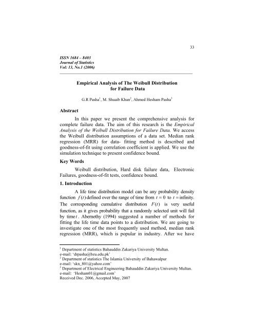
<strong>Empirical</strong> <strong>Analysis</strong> <strong>of</strong> <strong>The</strong> <strong>Weibull</strong> <strong>Distribution</strong> <strong>for</strong> <strong>Failure</strong> <strong>Data</strong> 33<br />
ISSN 1684 – 8403<br />
Journal <strong>of</strong> Statistics<br />
Vol: 13, No.1 (2006)<br />
________________________________________________________________<br />
<strong>Empirical</strong> <strong>Analysis</strong> <strong>of</strong> <strong>The</strong> <strong>Weibull</strong> <strong>Distribution</strong><br />
<strong>for</strong> <strong>Failure</strong> <strong>Data</strong><br />
G.R Pasha 1 , M. Shuaib Khan 2 , Ahmed Hesham Pasha 3<br />
Abstract<br />
In this paper we present the comprehensive analysis <strong>for</strong><br />
complete failure data. <strong>The</strong> aim <strong>of</strong> this research is the <strong>Empirical</strong><br />
<strong>Analysis</strong> <strong>of</strong> the <strong>Weibull</strong> <strong>Distribution</strong> <strong>for</strong> <strong>Failure</strong> <strong>Data</strong>. We access<br />
the <strong>Weibull</strong> distribution assumptions <strong>of</strong> a data set. Median rank<br />
regression (MRR) <strong>for</strong> data- fitting method is described and<br />
goodness-<strong>of</strong>-fit using correlation coefficient is applied. We use the<br />
simulation technique to present confidence bound.<br />
Key Words<br />
<strong>Weibull</strong> distribution, Hard disk failure data, Electronic<br />
<strong>Failure</strong>s, goodness-<strong>of</strong>-fit tests, confidence bound.<br />
1. Introduction<br />
A life time distribution model can be any probability density<br />
function f (t)<br />
defined over the range <strong>of</strong> time from t = 0 to t = infinity.<br />
<strong>The</strong> corresponding cumulative distribution F (t)<br />
is very useful<br />
function, as it gives probability that a randomly selected unit will fail<br />
by timet . Abernethy (1994) suggested a number <strong>of</strong> methods <strong>for</strong><br />
fitting the life time data points to a distribution. We are going to<br />
investigate one <strong>of</strong> the most frequently used method, median rank<br />
regression (MRR), which is popular in industry. After we have<br />
1 Department <strong>of</strong> statistics Bahauddin Zakariya University Multan.<br />
e-mail: ‘drpasha@bzu.edu.pk’<br />
2 Department <strong>of</strong> statistics <strong>The</strong> Islamia University <strong>of</strong> Bahawalpur<br />
e-mail: ‘skn_801@yahoo.com’<br />
3 Department <strong>of</strong> Electrical Engineering Bahauddin Zakariya University Multan.<br />
e-mail: ‘Hesham01@gmail.com’<br />
Received Dec. 2006, Accepted May, 2007
34<br />
Pasha, Khan, Pasha<br />
fitted the distribution to the data points we can then compute the<br />
parameters <strong>of</strong> that distribution using the MRR method. We can use<br />
the MRR method to solve <strong>for</strong> the parameters. <strong>The</strong> goodness-<strong>of</strong>-fit<br />
test can test whether the complete life data are from the weibull<br />
distribution or not. Abernethy and Fulton (1995, 96) idea are<br />
developed a graphical goodness-<strong>of</strong>-fit test. For a graphical<br />
goodness-<strong>of</strong>-fit test model uses the correlation coefficient (CC),<br />
which <strong>for</strong> the 2-parameter <strong>Weibull</strong> distribution, has been<br />
calculated. <strong>The</strong> resulting CC values can be used not only to<br />
compare fits by MRR methods but also to indicate how good a<br />
particular fit is. <strong>The</strong> primary advantage <strong>of</strong> <strong>Weibull</strong> analysis is the<br />
ability to provide reasonably accurate failure analysis and failure<br />
<strong>for</strong>ecasts with extremely small samples Chi-chao, (1997). Solutions<br />
are possible at the earliest indications <strong>of</strong> a problem without having<br />
to “crash a few more”. Another advantage <strong>of</strong> weibull analysis is<br />
that it provides a simple and useful graphical plot. In this paper the<br />
data plots are extremely important to the engineers.<br />
1.1 <strong>The</strong>oretical Background<br />
1.1.1 <strong>Weibull</strong> <strong>Distribution</strong><br />
<strong>The</strong> <strong>Weibull</strong> probability distribution has three parameters<br />
η, β andt 0<br />
. Abernthy 1994 express the shape and scale parameter<br />
<strong>of</strong> the <strong>Weibull</strong> distribution by W ( η,<br />
β ) . It can be used to represent<br />
the failure probability density function (PDF) with time, so it is<br />
defined as:<br />
f<br />
w<br />
( t)<br />
=<br />
t −t0<br />
β<br />
β t − t<br />
−(<br />
)<br />
0 β −1<br />
η<br />
(<br />
η<br />
η<br />
)<br />
e<br />
η > 0,<br />
β > 0, t<br />
0<br />
> 0,<br />
−∞ < t0<br />
< t (1)<br />
;<br />
Where β is the shape parameter (determining what the <strong>Weibull</strong><br />
PDF looks like) and is positive and η is a scale parameter<br />
(representing the characteristic life at which 63.2% <strong>of</strong> the<br />
population can be expected to have failed) and is also positive, t 0<br />
is a location or shift or threshold parameter (sometimes called a<br />
guarantee time, failure-free time or minimum life), t 0<br />
can be any<br />
real number, If t 0 then the <strong>Weibull</strong> distribution is said to be<br />
0 =
<strong>Empirical</strong> <strong>Analysis</strong> <strong>of</strong> <strong>The</strong> <strong>Weibull</strong> <strong>Distribution</strong> <strong>for</strong> <strong>Failure</strong> <strong>Data</strong> 35<br />
two-parameter Chi-chao, (1997). When β = 1, the distribution is the<br />
same as the exponential distribution <strong>for</strong> the density function.<br />
When β = 2 , it is known as the Rayleigh distribution <strong>for</strong> the<br />
density function. When β = 2. 5 , then the shape <strong>of</strong> the density<br />
function is similar to the Lognormal shape <strong>of</strong> function. When β =<br />
3.4 is then the shape <strong>of</strong> the density function is similar to the<br />
Normal shape <strong>of</strong> function<br />
2. Method <strong>of</strong> <strong>Analysis</strong><br />
2.1 Description <strong>of</strong> data<br />
Computer Hard Disk Drive <strong>Failure</strong>s data is taken to<br />
illustrate how to use the MRR methods, For the <strong>Empirical</strong><br />
<strong>Analysis</strong> <strong>of</strong> the <strong>Weibull</strong> <strong>Distribution</strong> <strong>for</strong> <strong>Failure</strong> <strong>Data</strong>. <strong>The</strong> data<br />
recorded the number <strong>of</strong> failures occurring within fixed time. <strong>The</strong><br />
t values in the data list represent actual time to failures life data<br />
in hours. <strong>The</strong>re are 16 Computer Hard Disk Drive <strong>Failure</strong>s life<br />
data Computer Hard Disk Drive <strong>Failure</strong>s “Source: Dev Raheja,<br />
Assurance Technologies”.<br />
2.2 <strong>Weibull</strong> <strong>Analysis</strong><br />
<strong>The</strong> <strong>Weibull</strong> cumulative distribution function (CDF),<br />
denoted by F(t), is:<br />
F<br />
w<br />
( t −t0<br />
β<br />
−<br />
η )<br />
( t ) = 1 − e<br />
(2)<br />
<strong>The</strong> liner <strong>for</strong>m <strong>of</strong> the resulting <strong>Weibull</strong> CDF can be<br />
represented by a rearranged version <strong>of</strong> equation (2):<br />
1 ⎛ 1 ⎞<br />
ln t = lnln + lnη<br />
β<br />
⎜<br />
1 () ⎟ ⎝ − FW<br />
t ⎠<br />
Comparing this equation with the liner <strong>for</strong>m y = Bx + A, leads to<br />
= and<br />
⎧ 1<br />
() ⎬ ⎫<br />
⎭<br />
y lnt x = ln ln⎨<br />
.<br />
⎩ 1−<br />
FW<br />
t<br />
If we minimize β and η by using the LS method then we obtain:
36<br />
Pasha, Khan, Pasha<br />
n<br />
n<br />
2 ⎛ ⎞<br />
n∑<br />
x<br />
i<br />
− ⎜ ∑ x<br />
i<br />
⎟<br />
ˆ<br />
i = 1 ⎝ i = 1<br />
β =<br />
⎠<br />
,<br />
(3)<br />
n<br />
n n<br />
n x y − x y<br />
∑<br />
i = 1<br />
i<br />
i<br />
∑<br />
i = 1<br />
∑<br />
i<br />
i = 1<br />
n<br />
n<br />
⎛<br />
⎞<br />
⎜ ∑ y<br />
i ∑ x<br />
i ⎟<br />
1<br />
1<br />
and ˆ exp ⎜ i =<br />
i =<br />
η =<br />
− ⎟,<br />
⎜ n n ˆ β ⎟<br />
⎜<br />
⎟<br />
⎝<br />
⎠<br />
2<br />
Where n is the sample size and ˆ indicates an estimate. <strong>The</strong><br />
mathematical expression <strong>for</strong> x<br />
i<br />
and y<br />
i<br />
are:<br />
⎡ 1 ⎤<br />
xi<br />
= ln ln⎢<br />
and y i<br />
= lnt<br />
i<br />
.<br />
⎣1−<br />
FW<br />
i<br />
( t ) ⎥ i ⎦<br />
i − 0.3<br />
F ( t i<br />
) can be estimated by using Benard’s <strong>for</strong>mula, ,<br />
n + 0.4<br />
which is a good approximation to the median rank estimator<br />
(Abernethy 1994 , Chi-chao, 1997, Tobias and Trindade 1986). We<br />
use the Benard’s median rank because it shows the best<br />
per<strong>for</strong>mance and it is the most widely used to estimate F ( t i<br />
). <strong>The</strong><br />
procedure <strong>for</strong> ranking complete data is as follows:<br />
1. List the time to failure data from small to large.<br />
2. Use Benard’s <strong>for</strong>mula to assign median ranks to each<br />
failure.<br />
3. Estimate the β and η by equations (3) and (4).<br />
<strong>The</strong> F ( t i<br />
) is estimated from the median ranks. Once â and bˆ<br />
are obtained, then βˆ and ηˆ can easily be obtained.<br />
3. <strong>Analysis</strong> Output and Result<br />
Computer Hard Disk Drive <strong>Failure</strong>s data is taken to<br />
illustrate how to use the MRR method. <strong>The</strong> <strong>Weibull</strong> method<br />
converting the recorded times into data points <strong>for</strong> linear<br />
regression using the above mention weibull analysis we per<strong>for</strong>m<br />
(4)
<strong>Empirical</strong> <strong>Analysis</strong> <strong>of</strong> <strong>The</strong> <strong>Weibull</strong> <strong>Distribution</strong> <strong>for</strong> <strong>Failure</strong> <strong>Data</strong> 37<br />
linear regressions <strong>for</strong> the data points. From the linear regression<br />
<strong>of</strong> weibull analysis we estimate β andη . <strong>The</strong>re are 16 Computer<br />
Hard Disk Drive <strong>Failure</strong>s life data shown as follows<br />
Fig.1 2-P <strong>Weibull</strong> <strong>Analysis</strong> <strong>for</strong> Hard Disk failure <strong>Data</strong><br />
Using <strong>Weibull</strong>++6 ηˆ = 366.2632, βˆ = 0.9207 and ρ = 0.9240<br />
can be readily obtained. Fig. 1 shows the Hard disk drive failures<br />
using MRR. <strong>The</strong> horizontal scale is a measure <strong>of</strong> failures life. <strong>The</strong><br />
vertical scale is the cumulative percentage failed .<strong>The</strong> two defining<br />
parameters <strong>of</strong> the weibull line are the slope, beta, and the<br />
characteristic life, eta. <strong>The</strong> slope <strong>of</strong> the line β is particularly<br />
significant and may provide a clue to the physics <strong>of</strong> the failure. We<br />
have age <strong>of</strong> the parts that are falling. Here age is the operating<br />
time. Here Beta
38<br />
Pasha, Khan, Pasha<br />
Fig.2 3-P <strong>Weibull</strong> <strong>Analysis</strong> <strong>for</strong> Hard Disk failure <strong>Data</strong><br />
Using <strong>Weibull</strong> Y-Bath TM ηˆ = 3080.9362 βˆ = 18.325231 and<br />
ˆt<br />
0<br />
= -2675.109 can be readily obtained. Fig. 2 shows the hard disk<br />
failures using MRR. Note that the final result <strong>of</strong> η must be<br />
adjusted <strong>for</strong> to t 0<br />
return to the original life scale, so ηˆ =<br />
3080.9362 -2675.109 = 405.8272. <strong>The</strong> result is ˆt 0<br />
= -2675.109<br />
when cc = 0.98594 reaches the maximum and the critical<br />
correlation coefficient ccc = 0.94739 Using a graphical method. In<br />
fig.2 the pattern <strong>of</strong> failure are closed to the estimated line. From<br />
this pattern it concludes that three parameter weibull distribution<br />
follow the hard disk failure data. Here ˆt 0<br />
< 0 it shows that concave<br />
is upward. From the linear regression <strong>of</strong> weibull analysis we<br />
estimate β andη . <strong>The</strong> slope and the y-intercept <strong>for</strong> the regression<br />
line <strong>of</strong> figure 1 are 0.9207and 366.2632 respectively. We then<br />
obtain the weibull parameters βˆ = 0.9207,ηˆ = 366.2632 and the<br />
correlation coefficient ρ = 0.9240. <strong>The</strong> weibull probability plot is<br />
obtained using <strong>Weibull</strong>++6 as shown in the following Figures from<br />
1 and 3-6. Here the horizontal scale is Hard disk <strong>Failure</strong> data in<br />
hour’s x .In figures (1) the vertical scale is the cumulative density
<strong>Empirical</strong> <strong>Analysis</strong> <strong>of</strong> <strong>The</strong> <strong>Weibull</strong> <strong>Distribution</strong> <strong>for</strong> <strong>Failure</strong> <strong>Data</strong> 39<br />
function (CDF), the proportion <strong>of</strong> the units that will fail up to age<br />
x in percent. <strong>The</strong> Statistical symbol <strong>for</strong> the CDF is F (x)<br />
, the<br />
probability <strong>of</strong> failure up to time x . Here in this graph the doted<br />
points which show the failure components. In figures (3) the<br />
vertical scale is the Value. In figures (4) the vertical scale is the<br />
failure rate (FR), <strong>The</strong> hazard function (HF) (also known as<br />
instantaneous failure rate), denoted by h(t), is defined as f(t)/R(t).<br />
<strong>The</strong> units <strong>for</strong> h(t) are probability <strong>of</strong> failure per unit <strong>of</strong> time, in<br />
hours. Here β < 1, the hazard function is continually decreasing<br />
which represents Infant Mortality. In figures (5) the horizontal<br />
scale is hard disk failure data in hours x . <strong>The</strong> vertical scale is the<br />
failure time line. In this graph the star line shows the failure<br />
component. In figures (6) the horizontal scale is eta the<br />
characteristic life (η ) and the vertical scale is beta ( β ) <strong>for</strong> the<br />
Contour <strong>Analysis</strong> <strong>for</strong> hard disk failure data. Here in these graph we<br />
find (99, 95, 90, 85, 75) ( 1 −α<br />
) percent confidence interval is the<br />
range <strong>of</strong> values, bounded above and below, within which the true<br />
value is expected to fall. It measures the statistical precision <strong>of</strong> our<br />
estimate. <strong>The</strong> probability that the true value lies within the interval<br />
is either zero or one, If we use 90% or above confidence interval<br />
then it will contain the true value <strong>for</strong> reliability intervals. Here the<br />
likelihood contour plots <strong>for</strong> the parameter eta and beta do not<br />
intersect; this would indicate significant differences with<br />
confidence levels. We have age <strong>of</strong> the hard disk failure data; here<br />
age is the operating time. Here Beta
40<br />
Pasha, Khan, Pasha<br />
Fig.3 2-p <strong>Weibull</strong> Histogram <strong>Analysis</strong> <strong>for</strong> Hard disk <strong>Failure</strong> data<br />
Fig.4 2-p <strong>Weibull</strong> <strong>Failure</strong> Rate <strong>Analysis</strong> <strong>for</strong> Hard disk <strong>Failure</strong> data
<strong>Empirical</strong> <strong>Analysis</strong> <strong>of</strong> <strong>The</strong> <strong>Weibull</strong> <strong>Distribution</strong> <strong>for</strong> <strong>Failure</strong> <strong>Data</strong> 41<br />
Fig.5 2-p <strong>Weibull</strong> Time <strong>Analysis</strong> <strong>for</strong> Engine fan life data<br />
Fig.6 2-p <strong>Weibull</strong> Contour <strong>Analysis</strong> <strong>for</strong> Hard disk <strong>Failure</strong> data<br />
<strong>The</strong> results <strong>of</strong> the sample about hard disk failure data using<br />
the MRR method are summarized in Table 1.
42<br />
Pasha, Khan, Pasha<br />
Table 1. Summary <strong>of</strong> results <strong>for</strong> hard disk failure data using<br />
MMR Method (n = 16)<br />
<strong>Distribution</strong>s<br />
<strong>Weibull</strong> <strong>Distribution</strong><br />
Method Parameters 2-P 3-P<br />
η 366.2632 3080.9362<br />
MRR β 0.9207 18.325231<br />
t<br />
0<br />
0 -2675.109<br />
Cc 0.9240 0.98594<br />
As we can see, the 3-parameter <strong>Weibull</strong> model CC =<br />
0.98594 show the curvature. But the 2-parameter <strong>Weibull</strong> plot do<br />
not show the curvature see Figure 1. Using the 2-parameter<br />
models, considering the 2-parameter <strong>Weibull</strong> CC = 0.9240. It<br />
follows that 3-p weibull gives consistent result than 2-p weibull<br />
distribution.<br />
3.1 Goodness-<strong>of</strong>-fit<br />
In statistics, there are many methods <strong>of</strong> measuring<br />
goodness-<strong>of</strong>-fit such as Anderson darling and kolmogorov<br />
simernov tests are applied but we prefer the simple correlation<br />
coefficient. It is ideal <strong>for</strong> testing the goodness <strong>of</strong> fit to a straight<br />
line. <strong>The</strong> correlation coefficient “r” is intended to measure the<br />
strength <strong>of</strong> a linear relationship between two variables. As <strong>Weibull</strong><br />
always have positive slopes, they will always have positive<br />
correlation coefficients. <strong>The</strong> closer “r” is to one the better the fit.<br />
<strong>The</strong> distribution <strong>of</strong> the correlation coefficient from ideal weibulls<br />
based on median rank plotting positions, For the 2-P <strong>Weibull</strong><br />
<strong>Analysis</strong> <strong>for</strong> Hard Disk failure <strong>Data</strong> Here coefficient <strong>of</strong><br />
determination r 2 = 0.85377< ccc =0.89169 so the fit is bad. While<br />
the 3-P <strong>Weibull</strong> <strong>Analysis</strong> <strong>for</strong> Hard Disk failure <strong>Data</strong> the coefficient<br />
<strong>of</strong> determination r 2 = 0.97207 > ccc =0.94739 so the fit is good.<br />
4. Conclusions<br />
<strong>The</strong> <strong>Weibull</strong> is extensively used in reliability and life<br />
testing. <strong>The</strong> weibull distribution is fitted the life data very well. We<br />
have concluded that while comparing this distribution <strong>for</strong> the two<br />
and three parameter, from the comparisons <strong>of</strong> the above results
<strong>Empirical</strong> <strong>Analysis</strong> <strong>of</strong> <strong>The</strong> <strong>Weibull</strong> <strong>Distribution</strong> <strong>for</strong> <strong>Failure</strong> <strong>Data</strong> 43<br />
here the three parameter weibull distribution provides better results<br />
than the two parameter <strong>Weibull</strong> distribution. But we also note that<br />
from the correlation coefficients the three parameter weibull<br />
distribution is consistent <strong>for</strong> the hard disk failure data.<br />
References:<br />
1. Abernathy, R. B. (1994). <strong>The</strong> New <strong>Weibull</strong> Handbook. SAE<br />
Pr<strong>of</strong>essional Development.<br />
2. Abernathy, R. B. and Fulton, W. (1995). <strong>Weibull</strong> NEWS. Fall.<br />
Abernathy, R. B. (2004). <strong>The</strong> New <strong>Weibull</strong> Handbook, 4th Edition,<br />
Dept. AT Houston, Texas 77252-2608, USA.<br />
3. Bain, L. J. (1978). Statistical <strong>Analysis</strong> <strong>of</strong> Reliability and Life-Testing<br />
Models: <strong>The</strong>ory and Methods, New York, USA.<br />
4. Berkson, J. (1950). Two Regressions Journal <strong>of</strong> the American<br />
Statistical Association. Vol. 45, (164-180).<br />
5. Lawless, J. F. (1982). Statistical Models and Methods <strong>of</strong> life<br />
time data, J WILEY, New York, USA.<br />
6. Liu, Chi-chao, (1997). A Comparison between the <strong>Weibull</strong> and<br />
Lognormal Models used to Analyze Reliability <strong>Data</strong>. P.hd thesis<br />
University <strong>of</strong> Nottingham, UK<br />
7. Schlitzer, L D. (1966) Monte Carlo Evaluation and<br />
Development <strong>of</strong> <strong>Weibull</strong> <strong>Analysis</strong> Techniques <strong>for</strong> Small Sample<br />
Sizes.<br />
8. Source <strong>of</strong> Computer Hard Disk Drive <strong>Failure</strong>s: Dev Raheja,<br />
Assurance Technologies.
44<br />
Pasha, Khan, Pasha<br />
APPENDIX<br />
Table A :<strong>Analysis</strong> <strong>of</strong> Hard Disk <strong>Failure</strong> <strong>Data</strong><br />
Time in P X<br />
hr<br />
7 0.042683<br />
12 0.103659<br />
49 0.164634<br />
140 0.22561<br />
235 0.286585<br />
260 0.347561<br />
320 0.408537<br />
320 0.469512<br />
380 0.530488<br />
388 0.591463<br />
437 0.652439<br />
472 0.713415<br />
493 0.77439<br />
524 0.835366<br />
529 0.896341<br />
592 0.957317<br />
For Two Parameter <strong>Weibull</strong> <strong>Distribution</strong> MRR<br />
Table B: 90% C.I <strong>for</strong> MRR in Monte Carlo <strong>Analysis</strong><br />
RUN r^2 ETA BETA<br />
Target 0.8537700 366.2632 0.9207271<br />
Lower 0.8598219 209.6378 0.5971654<br />
Upper 0.9944915 563.9925 1.4068030<br />
Table C: 95% C.I <strong>for</strong> MRR in Monte Carlo <strong>Analysis</strong><br />
RUN r^2 ETA BETA<br />
Target 0.8537700 366.2632 0.9207271<br />
Lower 0.8826149 180.4981 0.5927805<br />
Upper 0.9864513 634.3573 1.7665380
<strong>Empirical</strong> <strong>Analysis</strong> <strong>of</strong> <strong>The</strong> <strong>Weibull</strong> <strong>Distribution</strong> <strong>for</strong> <strong>Failure</strong> <strong>Data</strong> 45<br />
Table D: 99% C.I <strong>for</strong> MRR in Monte Carlo <strong>Analysis</strong><br />
RUN r^2 ETA BETA<br />
Target 0.8535761 366.5067 0.9178682<br />
Lower 0.8373939 177.2180 0.5272902<br />
Upper 0.9780507 566.5307 1.6812440<br />
For Three Parameter <strong>Weibull</strong> <strong>Distribution</strong> MRR<br />
Table E: 90% C.I <strong>for</strong> MRR in Monte Carlo <strong>Analysis</strong><br />
RUN r^2 To ETA BETA<br />
Target 0.9720674 -2675.109 3080.936 18.32523<br />
Lower -3.27274E+15 -45312.96 5.033961E-05 6.51398E-3<br />
Upper 1.11142E+15 776.7932 7.462147E+17 328.3123<br />
Table F: 95% C.I <strong>for</strong> MRR in Monte Carlo <strong>Analysis</strong><br />
RUN r^2 To ETA BETA<br />
Target 0.9720674 -2675.109 3080.936 18.32523<br />
Lower -1.04656E+15 -42812.13 281.3321 6.4677E-03<br />
Upper 3.132236E+14 746.8779 8.249263E+17 318.9428<br />
Table G :99% C.I <strong>for</strong> MRR in Monte Carlo <strong>Analysis</strong><br />
RUN r^2 To ETA BETA<br />
Target 0.9720674 -2675.109 3080.936 18.32523<br />
Lower -1.93351E+15 -1542434 176.3847 6.67443E-3<br />
Upper 1.454115E+14 657.758 2.813135E+17 10744.25