P3C: A New Algorithm for the Simple Temporal Problem

P 3 C: A New Algorithm for the Simple Temporal Problem
Léon Planken and Mathijs de Weerdt
Delft University of Technology, The Netherlands
{l.r.planken,m.m.deweerdt}@tudelft.nl
Abstract
The Simple Temporal Problem (STP) is a sub-problem of almost
any planning or scheduling problem involving time constraints.
An existing efficient method to solve the STP, called
△STP, is based on partial path consistency and starts from
a chordal constraint graph. In this paper, we analyse this
algorithm and show that there exist instances for which its
time complexity is quadratic in the number of triangles in the
constraint graph. We propose a new algorithm, P 3 C, whose
worst-case time complexity is linear in the number of triangles.
We show both formally and experimentally that P 3 C
outperforms △STP significantly.
Introduction
The Simple Temporal Problem (STP) was first proposed by
Dechter et al. (1991). The input to this problem is a set of
(time) variables with constraints that bound the difference
between pairs of these variables. The solution then is (an
efficient representation of) the set of all possible assignments
to these variables that meet these constraints, or the message
that such a solution does not exist.
The STP has received widespread attention that still lasts
today, with applications in such areas as medical informatics
(Anselma et al. 2006), spacecraft control and operations
(Fukunaga et al. 1997), and air traffic control (Buzing
and Witteveen 2004). Moreover, the STP appears as a pivotal
subproblem in more expressive formalisms for temporal
reasoning, such as the Temporal Constraint Satisfaction
Problem—proposed by Dechter et al. in conjunction with the
STP—and the Disjunctive Temporal Problem (Stergiou and
Koubarakis 2000). For our purposes, we will focus on the
importance of the STP for temporal planning (Nau, Ghallab,
and Traverso 2004, Chapter 15).
Traditionally, planning has been concerned with finding
out which actions need to be executed in order to achieve
some specified objectives. Scheduling was confined to finding
out when the actions need to be executed, and using
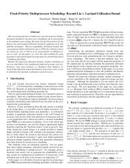
which resources. A typical architecture exploiting this separation
is presented in Figure 1: the first step separates the
causal information from the temporal information, resulting
in a classical planning problem that is solved with a classical
Copyright c○ 2008, Association for the Advancement of Artificial
Intelligence (www.aaai.org). All rights reserved.
Roman van der Krogt
Cork Constraint Computation Centre, Ireland
roman@4c.ucc.ie
Temporal information
Temporal problem Temporal domain
Classical problem
Translator
Planner
Partial Order Plan
Temporal Plan
Classical domain
Simple Temporal Problem
Figure 1: A typical architecture separating planning and
scheduling. Adapted from (Halsey, Long, and Fox 2004).
planner. This is then combined with the temporal information
that was removed during the first step to produce a temporal
plan. This approach is for example taken by McVey et
al. (1997). 1
However, in reality, planning and scheduling are intertwined:
time constraints affect which actions may be chosen,
and also how they should be combined. In such cases
the architecture of Figure 1 may not produce valid plans in
all occasions. The Crikey planner (Halsey, Long, and Fox
2004) circumvents this problem by identifying which parts
are separable, and which are not. In the parts that are nonseparable
the causal and temporal problems are solved together;
the separable parts are treated as separate problems.
Whereas Crikey tries to decouple planning and scheduling
as much as possible, other people have taken an iterative
approach. Both (Myers and Smith 1999) and (Garrido
and Barber 2001) discuss this type of approach in general.
1 Application of the architecture sketched here is not limited
to scheduling over time; Srivastava, Kambhampati, and Do (2001)
propose a similar architecture to schedule over the available resources.

A specific example of the approach is Machine T (Castillo,
Fdez-Olivares, and González 2002). Machine T is a partialorder
causal link planner that interleaves causal planning
with temporal reasoning. The temporal reasoning module
works on an STP instance that represents the partial plan of
the causal planner. It propagates time constraints, can be
used to identify threats by finding actions that possibly overlap
in time, and ensures consistency. The same approach is
taken by VHPOP (Younes and Simmons 2003).
Especially in the latter iterative approaches, the efficiency
with which STPs allow temporal information to be dealt
with is an important feature. For large problems, millions
of partial plans may be generated, and for each of those the
STP has to be updated and checked for consistency. In order
not to become a bottle-neck, the STP has to be solved very
quickly. The best known algorithm for STPs is called △STP
(pronounced triangle-STP) (Xu and Choueiry 2003). It requires
that the network be represented by a chordal graph.
Once a chordal graph is obtained (for which efficient heuristics
exist), △STP may require time quadratic in the number
of triangles in the graph, as we will prove below. Analysis of
this proof allows us to develop a new algorithm, called P 3 C,
which is linear in the number of triangles. This P 3 C algorithm
and the analysis of △STP are the main contributions
of this paper.
The remainder of the text is organised as follows. First,
we formally discuss the Simple Temporal Problem and describe
the existing solution techniques, including △STP.
Then, we analyse △STP and propose our new algorithm
P 3 C. After experimentally validating our method, we conclude.
The Simple Temporal Problem
In this section, we briefly introduce the Simple Temporal
Problem (STP); for a more exhaustive treatment, we refer
the reader to the seminal work by Dechter, Meiri, and
Pearl (1991).
An STP instance S consists of a set X = {x1,...,xn} of
time-point variables representing events, and a set C of m
constraints over pairs of time points, bounding the time difference
between events. Every constraint ci→j has a weight
wi→j ∈ R corresponding to an upper bound on the time difference,
and thus represents an inequality xj − xi ≤ wi→j.
Two constraints ci→j and cj→i can be combined into a single
constraint ci↔j : −wj→i ≤ xj − xi ≤ wi→j or, equivalently,
xj − xi ∈ [−wj→i,wi→j], giving both upper and
lower bounds. An unspecified constraint is equivalent to a
constraint with an infinite weight; therefore, if ci→j exists
and cj→i does not, we have ci↔j : xj − xi ∈ [−∞,wi→j].
The following planning problem will be used to illustrate
how an STP may arise as a sub-problem from a planning
problem. The resulting STP in this case is similar to the one
provided in (Dechter, Meiri, and Pearl 1991).
Example. The example deals with planning for an industrial
environment, including rostering and production planning.
For the purpose of this example, consider a situation
in which large parts of the plan have been computed already.
To get a fully working plan, all that remains to be done is to
x0
[10, 20]
x1
x3
[0, 20]
[50, 70]
[30, 40]
[40, 50]
Figure 2: An example STP instance S
d
d e
a b c a b c
(i) a wrapper (ii) clips
Figure 3: Two ways to encode time constraints. The wrapper
(i) encodes a time window within which the actions a,
b and c have to take place. Alternatively, constraints on the
interval allowed between two actions can be encoded using
clips (ii). Adapted from (Cresswell and Coddington 2003).
ensure that at any time an operator is assigned to monitor
the casting process. However, as casting is a relatively
safe process, it can be left unattended for at most 20 minutes
(between operator shifts). Moreover, the monitoring room is
small, and has room for just one person.
There are two operators available that can be assigned to
the casting task: John and Fred. Today, Fred’s shift must
end between 7:50 and 8:10. However, before he leaves, he
has to attend to some paperwork, which takes 40–50 minutes.
John is currently assigned to another task that ends
between 7:10 and 7:20. As it is located on the far side of the
plant, it will take him 30–40 minutes to make his way down
to the casting area.
The planning software generates a partial plan that lets
Fred start his shift at the casting process, with John taking
over after Fred leaves for his paperwork. The question now
is: is this a viable plan, and if so, what are the possible times
to let Fred stop, and let John start monitoring the casting
process?
To see how a Simple Temporal Problem can be used to
find the answer to our question, we first have to assign timepoint
variables to each event in the plan: let x1 and x2 represent
John leaving his previous activity and arriving at the
casting process, respectively; and let x3 and x4 denote
Fred starting his paperwork, and finishing it. A temporal
reference point, denoted by x0, is included to enable us to
refer to absolute time. For our example, it is convenient to
take x0 to stand for 7:00. If we represent all time intervals
in minutes, the graph representation of the STP for this example
is given in Figure 2; here, each vertex represents a
time-point variable, and each edge represents a constraint.
When represented as a graph in this way, the STP is also
referred to as a Simple Temporal Network (STN); however,
these terms are often used interchangeably.
It should be clear that the problem can arise from a PDDL
x2
x4

x0
[10, 20]
[20, 30]
x1
x3
[40, 50]
[10, 20]
[60, 70]
[50, 60]
[30, 40]
[10, 20] [20, 30]
[40, 50]
Figure 4: The minimal network M corresponding to S
planning description of the overall problem. Durative actions
with variable durations can be used to model the various
activities and a “wrapper” or a “clip” (Cresswell and
Coddington 2003) can be used to ensure that the process
does not go without an operator for more than 20 minutes
(see Figure 3).
Note that intervals labelling constraints can be used to
represent both freedom of choice for the actors (e.g. John’s
departure from his previous activity) as well as uncertainty
induced by the environment (e.g. travelling time). The approach
presented in this paper applies to both interpretations;
however, uncertainties can only be dealt with at plan
execution time, see e.g. (Vidal and Bidot 2001).
A solution to the STP instance is an assignment of a real
value to each time-point variable such that the differences
between each constrained pair of variables fall within the
range specified by the constraint. For example, the reader
can verify both from the network and from the original plan
that 〈x0 =0,x1 =10,x2 =40,x3 =20,x4 =70〉 is a
solution to our example STP. Note that many solutions exist;
to capture all of them, we are interested in calculating an
equivalent decomposable STP instance, from which all solutions
can then be extracted in a backtrack-free manner. The
traditional way to attain decomposability is by calculating
the minimal network M. InM, all constraint intervals have
been tightened as much as possible without invalidating any
solutions from the original instance.
The minimal network of our example is depicted in Figure
4. Note that some previously existing constraints have
been tightened; also, since the graph is now complete, new
information has become available. In the remainder of this
text, we will not concern ourselves with finding individual
solutions, but focus on finding decomposable networks
such as M from which such solutions can be efficiently extracted.
Such a network of minimal constraints is especially
useful when further additions of constraints are expected,
such as in the process of constructing a plan, because checking
whether a new constraint is consistent with the existing
ones can be done in constant time. Subsequently adapting
the constraints in a constraint network may cost more time.
Developing an efficient incremental algorithm to this end is
outside the scope of this paper, but an interesting and important
topic for further study.
x2
x4
1
2
3
4
5
6
7
8
9
Algorithm 1: DPC
Input: An STN instance S = 〈V,E〉 and an ordering
d =(vn,vn−1,...,v1)
Output: CONSISTENT or INCONSISTENT
for k ← n to 1 do
forall i, j < k such that {i, k}, {j, k} ∈E do
wi→j ← min(wi→j,wi→k + wk→j)
if wi→j + wj→i < 0 then
return INCONSISTENT
end
end
end
return CONSISTENT
Previous Solution Techniques
Dechter et al. noted (1991) that the Floyd-Warshall all-pairsshortest-paths
(APSP) algorithm can be used to compute the
minimal network M. Floyd-Warshall is simple to implement
and runs in O � n 3� time, where n is the number of
time-point variables in the STP instance. It corresponds to
enforcing the property of path consistency (PC) (Montanari
1974), known from constraint satisfaction theory.
For checking whether an STP instance is consistent,
Dechter et al. proposed directed path consistency (DPC),
which we include as Algorithm 1. The algorithm iterates
over the variables along some ordering d. After iteration k,
there exists an edge {vi,vj}, possibly added in line 3, for
every pair of nodes that are connected by a path in the subgraph
induced by {vk ∈ V | k>max(i, j)} ∪{vi,vj};
moreover, this edge is labelled by the shortest path in that
subgraph. This implies in particular that c1↔2 (if it exists)
is minimal. The algorithm runs in time O � n · (w ∗ (d)) 2� ,
where w ∗ (d) is a measure called the induced width relative
to the ordering d of the vertices in the constraint graph. For
d =(vn,vn−1,...,v1), wehave
w ∗ (d) = max|{{vi,vj}
∈E | j3 is a cycle, then any
edge on two nonadjacent vertices {vi,vj} with 1

Algorithm 2: △STP
Input: A chordal STN S = 〈V,E〉
Output: The PPC network of S or INCONSISTENT
1
2
3
4
5
6
7
8
9
10
11
12
13
14
Q ← all triangles in S
while Q �= ∅ do
choose T ∈ Q
foreach permutation (vi,vj,vk) of T do
wi→k ← min(wi→k,wi→j + wj→k)
if wi→k has changed then
if wi→k + wk→i < 0 then
return INCONSISTENT
end
Q ← Q ∪{all triangles ˆ T in S|vi,vk ∈ ˆ T }
end
end
Q ← Q \ T
end
Chordal graphs generally contain far less edges than complete
graphs; this holds especially if the graph was originally
sparse. Hence, enforcing PPC is often far cheaper than is enforcing
PC. Bliek and Sam-Haroud further proved that, for
convex problems, PPC produces a decomposable network
just like PC does.
Xu and Choueiry (2003) realised that the STP is a convex
problem, since each of its constraints is represented by
a single interval. Enforcing PPC on an STP instance then
corresponds to calculating the minimal labels for each edge
in the constraint graph, disregarding directionality. They implemented
an efficient version of the PPC algorithm, called
△STP, which we include as Algorithm 2.
The trade-off for the efficiency gained by enforcing PPC
is that less information is produced: whereas PC yields minimal
constraints between each pair of time-point variables,
PPC only labels the edges in the chordal graph with minimal
constraints. However, it can easily be ensured that all
information of interest is produced by adding new edges to
the constraint graph before triangulation. For this reason,
enforcing PPC can truly be seen as PC’s replacement for
solving the STP.
Xu and Choueiry show empirically that the △STP outperforms
the original PPC algorithm by Bliek and Sam-
Haroud, but they do not give a formal analysis of the time
complexity of △STP. In the next section we give an analysis,
showing that there exist problem instances for which
the time complexity of △STP is quadratic in the number of
triangles in the chordal constraint graph.
Worst-Case Analysis of △STP
Giving a tight bound on △STP’s time complexity in terms
of the number of variables or constraints in the STP instance
is not straightforward. However, looking at Algorithm 2, it
can be seen that the time complexity mainly depends on the
number of triangles t in the chordal STN that is the input
of the algorithm. In a way, this number t represents the difficulty
of the problem at hand. Note that there is no fixed
0
x7
τ1
1
0
5
τ2
2
x6
4
τ3
3
0
x0 x1 x2 x3
τ4
x5
0 0 0
Figure 5: Pathological test case P6 for △STP
3
4
2
τ5
path weight
∞
5
4
3
2
1
0
x0 → x7
x0 → x1 → x7
x0 → x1 → x6 → x7
x0 → x1 → x2 → x6 → x7
x0 → x1 → x2 → x5 → x6 → x7
x0 → x1 → x2 → x3 → x5 → x6 → x7
x0 → x1 → x2 → x3 → x4 → x5 → x6 → x7
Table 1: Total weights of paths in P6
relation between t and the size of the input except that there
is an upper bound of O � n3� , attained for a complete graph.
In this section we give a class P of pathological STP instances
for which the time complexity of △STP is quadratic
in the number of triangles. These instances have a constraint
graph consisting of a single directed cycle with all
zero weight edges; this cycle is filled with edges having carefully
selected weights. Before formally defining class P,we
include instance P6 as an example in Figure 5; its triangles
are labelled τ1 through τ6 for ease of reference.
Definition 2. The class P consists of pathological STP instances
Pt on t triangles for every t ∈ N. Each instance Pt
is defined on t +2variables {x0,x1,...,xt+1} and has the
following constraints (where xt+2 wraps around to x0):
•{ci→i+1 | 0 ≤ i ≤ t +1} with zero weight;
•{ci→j | 1 ≤ i ≤ j − 2

wt→1 is set to 0. This process is repeated until triangle τt
has been processed; at this point, all edges making up τt
have minimal weights, and we have that Q =(τ1,...,τt−1).
The algorithm starts again at triangle τ1 and proceeds to triangle
τt−1, after which Q =(τ1,...,τt−2). By now, the
pattern is clear: the total number of triangles processed is
t +(t − 1) + ···+1 = t(t +1)/2, which is indeed quadratic
in t.
These cases make it clear that the sequence in which
△STP processes the triangles in a constraint graph is not
optimal. It may be worthwhile to explore if there is a natural
way to order triangles in a chordal graph. For this reason,
we now turn to some theory concerning chordal graphs.
Graph Triangulation
In this section, we list some definitions and theorems from
graph theory which underlie the new algorithm we propose
in the next section. These results are readily available in
graph-theoretical literature, e.g. (West 1996).
Definition 3. Let G = 〈V,E〉 be an undirected graph. We
can define the following concepts:
• A vertex v ∈ V is simplicial if the set of its neighbours
Nv = {w | {v, w} ∈ E} induces a clique, i.e.
if ∀{s, t} ⊆Nv : {s, t} ∈E.
• Let d =(vn,...,v1) be an ordering of V . Also, let Gi
denote the subgraph of G induced by Vi = {v1,...,vi};
note that Gn = G. The ordering d is a simplicial elimination
ordering of G if every vertex vi is a simplicial vertex
of the graph Gi.
We then have the following (known) result:
Theorem 2. An undirected graph G = 〈V,E〉 is chordal if
and only if it has a simplicial elimination ordering.
In general, many simplicial elimination orderings exist.
Examples of such orderings for the graph depicted
in Figure 5 are (x0,x7,x1,x6,x2,x5,x3,x4) and
(x4,x0,x3,x5,x7,x2,x6,x1). 3
Chordality checking can be done efficiently in O (n + m)
time (where n = |V | and m = |E|) by the maximum cardinality
search algorithm. This algorithm iteratively labels
vertices with the most labeled neighbours, whilst checking
that these neighbours induce a clique. At the same time, it
produces (in reverse order) a simplicial elimination ordering
if the graph is indeed chordal.
If a graph is not chordal, it can be made so by the addition
of a set of fill edges. These are found by eliminating the
vertices one by one and connecting all vertices in the neighbourhood
of each eliminated vertex, thereby making it simplicial;
this process thus constructs a simplicial elimination
ordering as a byproduct. If the graph was already chordal,
following its simplicial elimination ordering means that no
fill edges are added. In general, it is desirable to achieve
chordality with as few fill edges as possible.
3 Like Xu and Choueiry, we disregard graph directionality
when discussing chordal STNs.
1
2
3
4
5
6
7
8
9
Algorithm 3: P 3 C
Input: A chordal STN S = 〈V,E〉 with a simplicial
elimination ordering d =(vn,vn−1,...,v1)
Output: The PPC network of S or INCONSISTENT
call DPC(S,d)
return INCONSISTENT if DPC did
for k ← 1 to n do
forall i, j < k such that {i, k}, {j, k} ∈E do
end
end
return S
wi→k ← min(wi→k,wi→j + wj→k)
wk→j ← min(wk→j,wk→i + wi→j)
Definition 4 (Kjærulff). Let G = 〈V,E〉 be an undirected
graph that is not chordal. A set of edges T with T ∩ E = ∅
is called a triangulation if G ′ = 〈V,E ∪ T 〉 is chordal. T is
minimal if there exists no subset T ′ ⊂ T such that T ′ is a
triangulation. T is minimum if there exists no triangulation
T ′ with |T ′ | < |T |.
Determining a minimum triangulation is an NP-complete
problem; in contrast, a (locally) minimal triangulation can
be found in O (nm) time (Kjærulff 1990). Since finding
the smallest triangulations is so hard, several heuristics have
been proposed for this problem. Kjærulff has found that both
the minimum fill and minimum degree heuristics produce
good results. The minimum fill heuristic always selects a
vertex whose elimination results in the addition of the fewest
fill edges; it has worst-case time complexity O � n 2� . The
minimum degree heuristic is even simpler, and at each step
selects the vertex with the smallest number of neighbours; its
complexity is only O (n), but its effectiveness is somewhat
inferior to that of the minimum fill heuristic.
The New Algorithm
Given a chordal graph with t triangles, the best known
method for enforcing partial path consistency (PPC) is the
△STP algorithm. As we demonstrated in Theorem 1, this
algorithm may exhibit time complexity Ω � t2� . In this section
we propose an algorithm that instead has time complexity
O (t): it enforces PPC by processing every triangle exactly
twice. To achieve this result, the simplicial elimination
ordering d must be known; as we stated in the previous section,
this is a byproduct of triangulation. Our new algorithm
is called P3C and is presented as Algorithm 3. It consists of
a forward and backward sweep along d. The forward sweep
is just DPC (see Algorithm 1); note that because d is simplicial,
no edges will be added. We now state the main results
of this paper.
Theorem 3. Algorithm P3C achieves PPC on consistent
chordal STNs.
Proof. Recall that for the STN, enforcing PPC corresponds
to calculating the shortest path for every pair of nodes connected
by an edge, i.e. calculating minimal constraints.

The algorithm first enforces DPC along d; thus, after this
step, there exists an edge {vi,vj} for every pair of nodes
that are connected by a path in the subgraph induced by
{vk ∈ V | k>max(i, j)} ∪{vi,vj}; moreover, this edge
is labelled by the shortest path in that subgraph. This means
in particular that c1↔2 (if it exists) is minimal.
It can now be shown by induction that after iteration k
of the forward sweep (lines 3–8), all edges in the subgraph
Gk induced by {vi ∈ V | i ≤ k} are labelled with minimal
constraint weights. The base case for k ≤ 2 has already been
shown to hold; assuming that the proposition holds for k−1,
we show that it also holds for k. Consider any constraint
ck→i with i

time [s]
0.4
0.35
0.3
0.25
0.2
0.15
0.1
0.05
P 3 C
ΔSTP
0
0 1000 2000 3000 4000 5000 6000 7000 8000 9000
triangles
Figure 8: Performance of △STP and P 3 C on job-shop
benchmarks
measured the time required to complete a run of the algorithms
proper; i.e., the triangulation of the constraint graphs
was excluded from the measurements.
For the evaluation of the pathological cases from Definition
2, we opted to include the Floyd-Warshall APSP algorithm.
The results are included in Figure 7. For this specifically
crafted category of problem instances, in which the
number of triangles is directly proportional to the number
of vertices, the performance of the three algorithms closely
follows the theoretical analysis. Floyd-Warshall exhibits
performance cubic in the number of triangles, △STP is
quadratic, and our new P 3 C algorithm remains linear in the
amount of triangles, as was proven above.
The instances of the job-shop problem we considered are
taken from the SMT-LIB benchmark library (Ranise and
Tinelli 2003). In effect, these are instances of the NP-hard
Disjunctive Temporal Problem (DTP): each constraint is a
disjunction of temporal inequalities. We generated a set of
STP instances by randomly selecting a single temporal inequality
from each disjunction. If such a component STP
were found to be consistent, it would constitute a solution
to the job-shop problem; combined with the size of the DTP
instances, this makes it highly unlikely that a random selection
yields a consistent STP instance. Nevertheless, these
instances can be considered representative of the types of
problems that an STP solver may be expected to deal with
as part of a planning algorithm that can deal with time.
In Figure 8, we include the results of running P 3 C and
△STP on STP instances generated in this fashion. The
jump that was already noticed in Figure 6 reappears in this
figure. Note, however, that across this jump the run time
does not keep pace with the number of triangles. Clearly,
the number of triangles in the problem instance is not the
only factor that determines problem complexity; recall that
the number of vertices and constraint edges only gradually
increase over the gap. We also observe that △STP does not
display a run time that is quadratic in the number of triangles
for these problem instances; as a consequence, the difference
between the results is much closer. However, P 3 C can still
time [s]
6
5
4
3
2
1
P 3 C
ΔSTP
0
0 500 1000 1500 2000 2500
triangles
Figure 9: Performance of △STP and P 3 C on job-shop
benchmarks with enforced consistency
clearly be seen to outperform its predecessor.
Running the algorithms on inconsistent instances is not a
full test of their prowess, because inconsistency is generally
discovered rather early along the way of calculating minimal
constraints; in the case of P 3 C, any inconsistency is
guaranteed to be found within the first loop. For this reason,
we randomly relabeled the constraint edges in the job-shop
STP instances in such a way that consistency was guaranteed,
and then ran the algorithms. The results of these tests
are depicted in Figure 9. Calculating minimal constraints
takes much more time than finding an inconsistency; for this
reason, we only included the smaller problem instances (up
to 2500 instead of 9000 triangles). Again, we can conclude
that our P 3 C algorithm consistently outperforms △STP,
though the results are somewhat closer than for the inconsistent
STPs. Finally, note that the performance of P 3 C is not
exactly linear in the amount of triangles for these test cases.
This is probably due to the overhead incurred by the used
data structures (hash tables), which were implicitly assumed
to have constant-time access in the theoretical analysis.
Conclusions and Future Research
We have taken a look at existing solution techniques for the
Simple Temporal Problem, and identified a class P of problem
instances for which the best existing algorithm △STP
exhibits a time complexity quadratic in the number of triangles.
By visiting the triangles in a specific order in a new
algorithm, called P 3 C, we showed that we can solve STP
within a time bounds linear in the number of triangles. This
so-called simplicial elimination ordering is a byproduct of
the triangulation phase, and therefore does not require any
additional calculations compared to △STP.
We corroborated our theoretical results with experiments
that included instances from both P and a more realistic set
of job-shop benchmarks. Throughout our experiments, P 3 C
clearly and consistently outperformed △STP. Future work
may evaluate the algorithms in a wider range of practical
settings.

Sometimes, it suffices to just determine consistency of the
STP. In these cases, instead of enforcing PPC, one can use
the Bellman-Ford algorithm, which runs in O (nm) time.
Although in the worst case this yields the same time complexity
as P 3 C, we have seen in a separate study that it is
faster on some of our benchmark problems. However, P 3 C
also yields minimal constraints, which is very useful in the
context of planning: here, the additional information about
remaining slackness is often more important than just knowing
whether the plan is consistent.
We expect that with little extra work, the results attained
here extend to general constraint satisfaction problems. The
original work on PPC by Bliek and Sam-Haroud had this
wider scope, but in the proof of P 3 C’s soundness we chose
to focus only on the STP, this being our subject of interest.
Future research will have to determine whether the algorithm
can indeed be applied in the context of general CSPs,
which would mean that our work also becomes of interest to
the CSP community.
Another line of future work comes from the observation
that using P 3 C, the worst-case complexity for establishing
PPC is of the same order as the worst-case complexity for
determining a minimal triangulation. It is worthwhile to
investigate the trade-off between, on the one hand, faster
triangulation (e.g. by relaxing the condition of minimality)
implying worse run time of the P 3 C algorithm, and, on the
other hand, better but slower triangulation yielding faster run
time of P 3 C.
Finally, we plan to propose an incremental PPC algorithm
in a future publication, building on the properties of chordal
graphs already explored here. An incremental solver takes
as input a partially path-consistent STP instance and a new
constraint to be added or an existing constraint to be tightened;
it then reports whether the new constraint still yields
a consistent instance and, if so, enforces PPC again. This is
especially useful for dealing with more complex (planning)
problems which require solving many, progressively larger
instances of the STP.
References
Anselma, L.; Terenziani, P.; Montani, S.; and Bottrighi, A.
2006. Towards a comprehensive treatment of repetitions,
periodicity and temporal constraints in clinical guidelines.
Artificial Intelligence in Medicine 38(2):171–195.
Bliek, C., and Sam-Haroud, D. 1999. Path consistency
on triangulated constraint graphs. In Proc. of the 16th Int.
Joint Conf. on Artificial Intelligence, 456–461. San Francisco,
CA, USA: Morgan Kaufmann Publishers Inc.
Buzing, P., and Witteveen, C. 2004. Distributed (re)planning
with preference information. In Verbrugge, R.;
Taatgen, N.; and Schomaker, L., eds., Proc. of the 16th
Belgium-Netherlands Conf. on AI, 155–162.
Castillo, L.; Fdez-Olivares, J.; and González, A. 2002.
A temporal constraint network based temporal planner.
In Proc. of the 21st Workshop of the UK Planning and
Scheduling Special Interest Group, 99–109.
Cresswell, S., and Coddington, A. 2003. Planning with
timed literals and deadlines. In Proc. of the Twenty-Second
Workshop of the UK Planning and Scheduling Special Interest
Group (PlanSIG-03), 22–35.
Dechter, R.; Meiri, I.; and Pearl, J. 1991. Temporal constraint
networks. Artificial Intelligence 49(1–3):61–95.
Dechter, R. 2003. Constraint Processing. San Francisco,
CA, USA: Morgan Kaufmann Publishers Inc.
Fukunaga, A.; Rabideau, G.; Chien, S.; and Yan, D. 1997.
Aspen: A framework for automated planning and scheduling
of spacecraft control and operations. In Proc. of the Int.
Symposium on AI, Robotics and Automation in Space.
Garrido, A., and Barber, F. 2001. Integrating planning and
scheduling. Applied Artificial Intelligence 15:471–491.
Halsey, K.; Long, D.; and Fox, M. 2004. CRIKEY – a
temporal planner looking at the integration of planning and
scheduling. In Proc. of the ICAPS 2004 Workshop on Integrating
Planning into Scheduling, 46–52.
Kjærulff, U. 1990. Triangulation of graphs - algorithms
giving small total state space. Technical report, Aalborg
University.
McVey, C. B.; Durfee, E. H.; Atkins, E. M.; and Shin, K. G.
1997. Development of iterative real-time scheduler to planner
feedback. In Proc. of the 15th Int. Joint Conf. on Artificial
Intelligence, 1267–1272.
Montanari, U. 1974. Networks of constraints: Fundamental
properties and applications to picture processing. Information
Science 7(66):95–132.
Myers, K., and Smith, S. 1999. Issues in the integration of
planning and scheduling for enterprise control. In Proc. of
the DARPA Symposium on Advances in Enterprise Control.
Nau, D.; Ghallab, M.; and Traverso, P. 2004. Automated
Planning: Theory & Practice. Morgan Kaufmann Publishers.
Ranise, S., and Tinelli, C. 2003. The SMT-LIB format: An
initial proposal. In Proceedings of PDPAR’03.
Srivastava, B.; Kambhampati, S.; and Do, M. B. 2001.
Planning the project management way: Efficient planning
by effective integration of causal and resource reasoning in
realplan. Artificial Intelligence 131(1–2):73–134.
Stergiou, K., and Koubarakis, M. 2000. Backtracking algorithms
for disjunctions of temporal constraints. Artificial
Intelligence 120(1):81–117.
Vidal, T., and Bidot, J. 2001. Dynamic sequencing of tasks
in simple temporal networks with uncertainty. In CP 2001
Workshop in Constraints and Uncertainty.
West, D. B. 1996. Introduction to Graph Theory. Prentice-
Hall.
Xu, L., and Choueiry, B. Y. 2003. A new efficient algorithm
for solving the Simple Temporal Problem. In Proc. of
the 10th Int. Symp. on Temporal Representation and Reasoning
and 4th Int. Conf. on Temporal Logic, 210–220.
IEEE Computer Society.
Younes, H. L. S., and Simmons, R. G. 2003. VHPOP:
Versatile heuristic partial order planner. Journal of AI Research
20:405–430.