Optimal Control for 2D Parabolic Problems
Optimal Control for 2D Parabolic Problems
Optimal Control for 2D Parabolic Problems

Create successful ePaper yourself
Turn your PDF publications into a flip-book with our unique Google optimized e-Paper software.
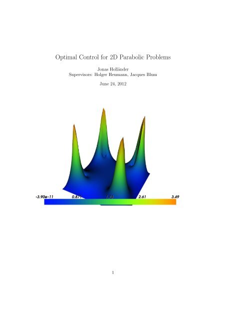
<strong>Optimal</strong> <strong>Control</strong> <strong>for</strong> <strong>2D</strong> <strong>Parabolic</strong> <strong>Problems</strong><br />
Jonas Holländer<br />
Supervisors: Holger Heumann, Jacques Blum<br />
June 24, 2012<br />
1
Contents<br />
1 Theory of the optimal control problem 2<br />
1.1 Introduction of the problem . . . . . . . . . . . . . . . . . . . . . . . . . . 2<br />
1.2 Discretization of the constraint . . . . . . . . . . . . . . . . . . . . . . . . 4<br />
1.3 Discretization of the costfunctional . . . . . . . . . . . . . . . . . . . . . . 4<br />
1.4 Set up of the Lagrangian and first order optimality conditions . . . . . . . 5<br />
1.5 Collecting the optimality conditions . . . . . . . . . . . . . . . . . . . . . 5<br />
2 Implementation of the <strong>Optimal</strong> <strong>Control</strong> Problem in Fenics 7<br />
2.1 Motivation to use Fenics . . . . . . . . . . . . . . . . . . . . . . . . . . . . 7<br />
2.2 Implementation of the domains and the boundaries . . . . . . . . . . . . . 7<br />
2.3 Implementation of the functionspace . . . . . . . . . . . . . . . . . . . . . 8<br />
2.4 Implementation of the boundary conditions . . . . . . . . . . . . . . . . . 9<br />
2.5 Implementation of the linear system and the initial conditions . . . . . . . 9<br />
2.6 Solving the linear system . . . . . . . . . . . . . . . . . . . . . . . . . . . 11<br />
3 Results 12<br />
3.1 Expected behavior of u and f . . . . . . . . . . . . . . . . . . . . . . . . . 12<br />
3.2 Comparison between expectation and model . . . . . . . . . . . . . . . . . 12<br />
3.3 Numerical limits . . . . . . . . . . . . . . . . . . . . . . . . . . . . . . . . 16<br />
4 Conclusion 17<br />
References 18<br />
1 Theory of the optimal control problem<br />
1.1 Introduction of the problem<br />
In this project we want to solve an optimal control problems like the one given through<br />
equations (1)-(5).<br />
∫ T<br />
min<br />
u(x,t),f(x,t) 0<br />
ω 1<br />
2 〈f(x, t), f(x, t)〉 Ω C<br />
+ ω 2<br />
2 〈u(x, t)−sin(2πt), u(x, t)−sin(2πt)〉 Ω P<br />
dt, (1)<br />
c(x) ∂ t u(x, t) − ∆u(x, t) = f(x, t) in Ω, (2)<br />
{ { ≠ 0 if x ∈ ΩC<br />
1 if x ∈ ΩC<br />
with f(x) =<br />
c(x) =<br />
= 0 else ,<br />
0 else ,<br />
(3)<br />
u(x, 0) = u 0 (x) in Ω, (4)<br />
u(x, t) = 0 on ∂Ω. (5)<br />
2
Figure 1: The definition of the domain of the optimal control problem<br />
Where the domains are defined through:<br />
Ω := [0, 1] × [0, 1],<br />
Ω P := [0.3, 07] × [0.25, 0.75],<br />
⎧<br />
[0.15, 0.25] × [0.1, 0.2]<br />
⎪⎨<br />
[0.15, 0.25] × [0.8, 0.9]<br />
Ω C :=<br />
[0.75, 0.85] × [0.1, 0.2]<br />
⎪⎩<br />
[0.75, 0.85] × [0.8, 0.9],<br />
(6)<br />
which means there are 2 functions searched, which are connected by a partial differential<br />
equation. This function should be furthermore the solution of a minimization problem.<br />
The domain we want to consider in our problem is divided into 5 subdomains:<br />
• The subdomain Ω 5 or Ω P is a rectangular centered in the middle of the domain. It<br />
is of interest since the second part of equation (1) just depends on these domain.<br />
• The subdomains Ω 1 , Ω 2 , Ω 3 and Ω 4 are part of the subdomain Ω C . These subdomains<br />
are small squares surrounding Ω P at the corners. The function f as well<br />
as the constant in front of the time derivative are just different from 0 inside this<br />
domain.<br />
The subdivision of the domain is illustrated in picture (1). We want to solve this problem<br />
with the help of finite element methods. This means we first want to write the discrete<br />
versions of the problem, and derive the Lagrangian of this discrete version. Afterwards we<br />
derivate the Lagrangian to achieve the first order optimality conditions. This conditions<br />
3
can be represented through a linear system, which was assembled and solved with the<br />
help of the program fenics. 1<br />
1.2 Discretization of the constraint<br />
We want to find a solution of this problem with the help of the finite element method.<br />
There<strong>for</strong> we introduce a discretization of space and time and write:<br />
f(x, t n ) =<br />
N∑<br />
fi n φ i (x) and u(x, t n ) =<br />
i=1<br />
N∑<br />
u n i φ i (x), (7)<br />
i=1<br />
where φ i (x) denotes one of the basisfunctions of the interpolationspace S. This discretization<br />
is applied to the weak <strong>for</strong>mulation of equation (2):<br />
∫<br />
∫<br />
c(x)∂ t u(x, t)ψ(x, t) + ∇u(x, t) · ∇ψ(x, t)dx = f(x, t)ψ(x, t)dx. (8)<br />
Ω<br />
We define 2 finite element matrices now through:<br />
∫<br />
∫<br />
∫<br />
c i,j := φ i (x)φ j (x)dx, m i,j := φ i (x)φ j (x)dx, k i,j :=<br />
Ω C Ω<br />
Ω<br />
Ω<br />
∇φ i (x) · ∇φ j (x)dx, (9)<br />
and use the notation of u n := (u n 1 , un 2 , ..., un I<br />
) to write the discrete version of equation<br />
(8) in the following way:<br />
v t C (un+1 − u n )<br />
δt<br />
+ v t Ku n+1 − v t Cf n = 0 ∀v ∈ R I . (10)<br />
Since this equation holds <strong>for</strong> any v ∈ R I , it holds especially <strong>for</strong> the basisvectors with<br />
which it holds <strong>for</strong> any component and we can write the equation without v t and we get<br />
our constraint:<br />
K n (u, f) := C (un − u n−1 )<br />
+ Ku n − Cf n = 0. (11)<br />
δt<br />
1.3 Discretization of the costfunctional<br />
The next step we have to go <strong>for</strong> computing the first order optimality condition is to<br />
determine the discrete version of the costfunctional given through equation (1). Here we<br />
use the discretization:<br />
J(u, f) :=<br />
N∑<br />
(f n ) t Mf n δtω 1<br />
2<br />
n=1<br />
+<br />
N∑<br />
(u n − sin(2πt n )) t P(u n − sin(2πt n )) δtω 2<br />
2 , (12)<br />
n=1<br />
where the Matrix P denote the components of 〈φ i , φ j 〉 ΩP .<br />
1 http://fenicsproject.org<br />
4
1.4 Set up of the Lagrangian and first order optimality conditions<br />
For computing the first order optimality conditions we set up the Lagrangian and compute<br />
the derivatives with respect to the components u, f and λ. The Lagrangian can be<br />
written in the <strong>for</strong>m:<br />
L(u, f, λ) = J(u, f) +<br />
N∑<br />
〈λ i , K n (u, f)〉. (13)<br />
From this equation we get the first order optimality conditions as the derivatives of<br />
L(u, f, λ) with respect to the variables u, f and λ. The derivative with respect to λ is<br />
given through equation (11). The optimality conditions are then:<br />
n=1<br />
∂L(u, f, λ)<br />
∂u i = ω 2 δtP(u i − sin(2πt i )) + G t λ i − 1 δt Ct λ i+1 = 0 ∀i ≠ n, (14)<br />
∂L(u, f, λ)<br />
∂u n = ω 2 δtP(u n − sin(2πt n )) + G t λ n = 0, (15)<br />
∂L(u, f, λ)<br />
∂f i = ω 1 δtMf i − C t λ i = 0, (16)<br />
∂L(u, f, λ)<br />
∂λ i = −C 1 δt ui−1 + Gu i − Cf i = 0, (17)<br />
where G was defined through G := 1 δt C + K.<br />
1.5 Collecting the optimality conditions<br />
The next step to take is to <strong>for</strong>m out of this equations a system of equation to be able<br />
to solve it with any linear solver. There<strong>for</strong> we collect all the terms of u, f and λ in a<br />
solution vector and get the following block matix:<br />
⎛ ⎞ ⎛<br />
u A 1 0 A t ⎞ ⎛ ⎞ ⎛ ⎞<br />
2 u 1<br />
A ⎝f⎠ = ⎝ 0 A 3 A t ⎠ ⎝<br />
4 f⎠ = ⎝b<br />
0 ⎠ , (18)<br />
λ A 2 A 4 0 λ b 2<br />
The matrices A 1 , A 3 and A 4 are again blockmatrices with only blocks on the diagonal,<br />
the matrix A 2 has a slightly different shape. All their <strong>for</strong>ms are given by:<br />
⎛<br />
⎞<br />
ω 2 δtP 0 . . . 0<br />
A 1 :=<br />
0 ω 2 δtP . . . .<br />
⎜<br />
⎝<br />
.<br />
. .. . ..<br />
⎟ 0 ⎠ , (19)<br />
0 . . . 0 ω 2 δtP<br />
5
⎛<br />
⎞<br />
G 0 . . . . . . 0<br />
−C 1 δt<br />
G . . .<br />
A 2 :=<br />
0 −C 1 δt<br />
G . . .<br />
. . .. . .. . .. . .. , (20)<br />
.<br />
⎜<br />
.<br />
⎝ .<br />
.. . .. . .. ⎟ 0 ⎠<br />
0 . . . . . . 0 −C 1 δt<br />
G<br />
⎛<br />
⎞<br />
ω 1 δtM 0 . . . 0<br />
A 3 :=<br />
0 ω 1 δtM . . . .<br />
⎜<br />
⎝<br />
.<br />
. .. . ..<br />
⎟ 0 ⎠ , (21)<br />
0 . . . 0 ω 1 δtM<br />
⎛<br />
⎞<br />
−C 0 . . . 0<br />
A 1 :=<br />
0 cC . . . .<br />
⎜<br />
⎝<br />
.<br />
. .. . ..<br />
⎟ 0 ⎠ . (22)<br />
0 . . . 0 −C<br />
It is here nice to notice that A is symmetric which means that A = A t because of the<br />
symmetry of A 1 and A 3 and of the structure and position of the other matrices.<br />
The vector b 1 is determined through equation (14) and (15), here the part −ω 2 δtPsin(2πt n )<br />
is not depending on u, f and λ and is there <strong>for</strong> moved to the right hand side of the equation.<br />
The other vector b 2 is almost every where 0. The first term depends on u 0 which<br />
is given through the initial conditions of optimal control problem. Since this term also<br />
not depends on any other components of u, f and λ it has to appear on the right side<br />
through 1 δt Cu0 .<br />
We find the desired solution u by solving the linear system (18).<br />
6
2 Implementation of the <strong>Optimal</strong> <strong>Control</strong> Problem in Fenics<br />
2.1 Motivation to use Fenics<br />
The biggest problem of solving equation (18) is the implementation of all the finite element<br />
matrices needed. This matrices make it hard to implement this problem in 1<br />
dimension and even more complicated to handle this problem in 2 or more dimensions.<br />
However, the <strong>for</strong>m of equation (18) will not change, just the submatrices inside change.<br />
To solve this problem we there <strong>for</strong> take the software fenics, since it makes the implementation<br />
incredibly much easier. This software has the idea to assemble in a easy way<br />
all the finite element matrices, apply the boundary conditions and solve the constructed<br />
linear system. Furthermore it allows us to define all the necessary subdomains and the<br />
right functionspaces.<br />
The last important reason <strong>for</strong> using fenics is the possibility to adapted the code fast to<br />
other optimal control problem, which would take without it incredible much time since<br />
it needs all the finite element matrices to be changed.<br />
2.2 Implementation of the domains and the boundaries<br />
The first necessary step to take in the implementation is the definition of the domains.<br />
We need to define a unit-square with the 5 subdomains Ω 1 to Ω 5 , to define the variational<br />
<strong>for</strong>mulation of our problem. To be able to solve our problem we need the appropriate<br />
boundary conditions, in our case Dirichlet boundary conditions, <strong>for</strong> which we need to<br />
define the boundary. All this is shown in the following lines of code exemplary <strong>for</strong> the<br />
left boundary and the domain Ω 1 :<br />
1<br />
# D e f i n i t i o n o f the domain and the f u n c t i o n s p a c e<br />
3 mesh = UnitSquare ( 6 4 , 64)<br />
5 c l a s s L e f t ( SubDomain ) :<br />
d e f i n s i d e ( s e l f , x , on boundary ) :<br />
7 r e t u r n near ( x [ 0 ] , 0 . 0 )<br />
9 c l a s s Areaone ( SubDomain ) :<br />
d e f i n s i d e ( s e l f , x , on boundary ) :<br />
11 r e t u r n ( between ( x [ 0 ] , ( 0 . 1 5 , 0 . 2 5 ) ) and between ( x [ 1 ] , ( 0 . 1 , 0 . 2 ) ) )<br />
Line 2 defines the mesh as a unit-square with 64 × 64 elements. In line 4 the initialization<br />
of the left boundary starts. It is define as all nodes of the mesh which have<br />
|x| < ɛ. It is not take the exact value x = 0 to prevent the loss of boundary points<br />
through rounding errors. We define the subdomain Ω 1 in a similar way in the area<br />
(0, 15 ≤ x ≤ 0, 25 × 0, 1 ≤ x ≤ 0, 2)<br />
7
After the initialization of the mesh function <strong>for</strong> the interior domains and boundaries,<br />
which is done in line 1-11 of the following code block. It is necessary to define symbolic<br />
measures <strong>for</strong> the domains and boundaries. This makes the process of creating the<br />
variational <strong>for</strong>mulation easier.<br />
1<br />
# I n i t i a l i z e mesh f u n c t i o n f o r i n t e r i o r domains<br />
3 domains = CellFunction ( ” u i n t ” , mesh )<br />
domains . s e t a l l ( 0 )<br />
5 areaone . mark ( domains , 1)<br />
7 # I n i t i a l i z e mesh f u n c t i o n f o r boundary domains<br />
boundaries = FacetFunction ( ” u i n t ” , mesh )<br />
9 boundaries . s e t a l l ( 0 )<br />
l e f t . mark ( boundaries , 1 )<br />
11<br />
# Define new measures a s s o c i a t e d with the i n t e r i o r domains and<br />
13 # e x t e r i o r boundaries<br />
dx = Measure ( ”dx” ) [ domains ]<br />
15 ds = Measure ( ” ds ” ) [ boundaries ]<br />
2.3 Implementation of the functionspace<br />
Our aim is to solve the optimal control problem in the space of continuous function.<br />
Because of this we want to chose Lagrange elements to interpolate our solution. Every<br />
time step we have to solve a linear system <strong>for</strong> the 3 unknowns u, f and λ, the problems<br />
<strong>for</strong> different time steps depend on each which makes it hard to solve them separately.<br />
To avoid this problem we convert it to a finite element problem of a vectorial function,<br />
where the components are one of the unknown functions u, f and λ at a certain timestep.<br />
The creation of this functionspaces is done in the programm through the following lines<br />
of code:<br />
1 #d e f i n i t i o n o f the f u n c t i o n s p a c e s<br />
V = FunctionSpace ( mesh , ’ Lagrange ’ , 1)<br />
3 S = MixedFunctionSpace ( [V] ∗ 3 ∗ number )<br />
u = T r i a l F u n c t i o n s ( S )<br />
5 v = TestFunctions ( S )<br />
The second line of codes defines the functionspace <strong>for</strong> one of the unknowns u, f or λ, and<br />
states that the space should be the space of first order Lagrange elements on the previous<br />
defined mesh. The next line defines the space of functions which we actually use, as the<br />
productspace of V 3N , with N as the number of time steps. In the last lines some trial and<br />
test functions are initialized, which are later necessary to define the variational problem.<br />
8
2.4 Implementation of the boundary conditions<br />
This subsection is on the implementation of the boundary conditions of our optimal<br />
control problem. The easiest boundary conditions applicable are Dirichlet boundary<br />
conditions and these are the ones we want to use. The problem here is to find the right<br />
boundary values since we are now in the space V 3N , which means we have to define<br />
boundary values <strong>for</strong> all components.<br />
The boundary values of all components associated to u are 0, because of equation (5).<br />
The values associated to f are 0, because of (3) and the fact that there is no intersection<br />
of Ω C and the boundary. That all components of λ are 0 comes from equation (14) and<br />
the fact that u = 0 on the boundary. Since it is now clear that all components vanish<br />
on the boundary, we can have a look at the implementation:<br />
1 #v e c t o r f o r the boundary c o n d i t i o n s<br />
vec = [ 0 . 0 ] ∗ 3 ∗ number<br />
3 # Define D i r i c h l e t boundary c o n d i t i o n s at top and bottom boundaries<br />
bcs = [ DirichletBC (S , vec , boundaries , 1) ,<br />
5 DirichletBC (S , vec , boundaries , 2) ,<br />
DirichletBC (S , vec , boundaries , 3) ,<br />
7 DirichletBC (S , vec , boundaries , 4) ]<br />
Here we do two things, first we create a vector with all components 0 and the appropriate<br />
size <strong>for</strong> our boundary conditions, second we create a list of boundary conditions. The<br />
components of the list are 0 boundary conditions, of the functionspace S applied to the<br />
boundaries 1-4. Where the numbers 1-4 correspond to the markings previously done.<br />
2.5 Implementation of the linear system and the initial conditions<br />
In this section I want to present the way equation (18) was inserted into Fenics. To<br />
illustrate this I will use the first line of equation (18):<br />
⎛ ⎞<br />
⎛ ⎞<br />
u<br />
B ⎝f⎠ = ( A 1 0 A t )<br />
u<br />
⎝<br />
2 f⎠ = b 1 . (23)<br />
λ<br />
λ<br />
The Matrix we want to consider has N ×3N components where each component contains<br />
a finite element matrix. The Matrix A 1 is a block diagonal Matrix with the Matrix ω 2 δtP<br />
on the diagonal. It is created through:<br />
1 #d e f i n i t i o n o f the matrix<br />
aa = omega2 ∗ dt ∗ dot ( u [ 0 ] , v [ 0 ] ) ∗dx ( 5 )<br />
3 #e n t e r i n g Matrix A 1<br />
f o r i i n range ( 1 , number ) :<br />
5 aa = aa + omega2 ∗ dt ∗ i n n e r ( u [ i ] , v [ i ] ) ∗dx ( 5 )<br />
9
The definition of aa contains the test and the trial function from which it is clear that<br />
we want to create a matrix. The part dot(u[0],v[0]) stands <strong>for</strong> the finite element matrix<br />
associated to mass matrix m in equation (9), and the two [0] indicate that it’s the 0/0<br />
block-matrix of the matrix B. The multiplication with dx(5) stands <strong>for</strong> integrating this<br />
part of the equation just over the domain marked with number 5, in our case P. In<br />
the loop afterwards all further matrices of A 1 are added. The implementation of the<br />
matrices A 2 is done similar by:<br />
1 #e n t e r i n g Matrix A 2t<br />
f o r i i n range ( number ) :<br />
3 f o r j i n range ( 6 ) :<br />
aa = aa + dot ( grad ( u [ i +2∗number ] ) , grad ( v [ i ] ) ) ∗dx ( j )<br />
5 f o r i i n range ( number ) :<br />
f o r j i n range ( 1 , 5 ) :<br />
7 aa = aa + (1/ dt ) ∗ dot ( u [ i +2∗number ] , v [ i ] ) ∗dx ( j )<br />
f o r i i n range ( number−1) :<br />
9 f o r j i n range ( 1 , 5 ) :<br />
aa = aa −(1/ dt ) ∗ dot ( u [ i +2∗number +1] , v [ i ] ) ∗dx ( j )<br />
The matrix A t 2 consists of 3 parts, 2 matrices on the diagonal blocks and one up the<br />
diagonal. The matrices on the diagonal blocks are added again in the same way, the 2<br />
differences are first the shifting of u by a factor of 2*number and second the different<br />
term in the first matrix. The command dot(grad(u),grad(v)) stands <strong>for</strong> another finite<br />
difference matrix, the last one given through equation (9). The last matrix up of the<br />
diagonal is implemented similar to the previous one, just with an additional factor of 1<br />
added to indicate that the different position. All the summations over j indicate over<br />
which domains the integration takes part, e.g. <strong>for</strong> the second and third matrices over<br />
Ω 1 to Ω 4 .<br />
The initial conditions we want to consider are given through:<br />
⎛ ⎞<br />
⎛ ⎞<br />
⎛<br />
1<br />
sin(2πt<br />
⎝b n ⎞<br />
1<br />
)<br />
δt Cu0<br />
0 ⎠ ⎜ ⎟<br />
0<br />
with b 1 := ω 2 δtP ⎝ . ⎠ and b 2 := ⎜ ⎟<br />
b 2 sin(2πt n ⎝ . ⎠ , (24)<br />
)<br />
0<br />
They are implemented via the following lines:<br />
#d e f i n i t i o n o f the i n i t i a l c o n d i t i o n s<br />
2 u0 = Expression ( ”− 10∗ exp(− pow( x [ 1 ] − 0 . 5 , 2) ) ” )<br />
f = (1/ dt ) ∗u0∗v [ 2 ∗ number ] ∗ dx ( 1 )+ (1/ dt ) ∗u0∗v [ 2 ∗ number ] ∗ dx ( 2 ) +(1/ dt ) ∗u0∗v<br />
[ 2 ∗ number ] ∗ dx ( 3 ) +(1/ dt ) ∗u0∗v [ 2 ∗ number ] ∗ dx ( 4 )<br />
4 f o r i i n range ( number ) :<br />
f = f +s i n (2∗ i ∗ dt ∗ 3 . 1 4 1 5 ) ∗omega2∗ dt ∗v [ i ] ∗ dx ( 5 )<br />
10
The second line gives the possibility to implement a function as initial conditions. In<br />
the next line a right hand side vector is created which contains b 2 . Afterwards the initial<br />
conditions <strong>for</strong> b 1 are set in a loop.<br />
It is to mention that we just have to change this part if we want to use the program to<br />
solve another optimal control problem in the same domain.<br />
2.6 Solving the linear system<br />
The last step left now is to solve the linear system. Here <strong>for</strong> we use the default solver of<br />
fenics UMFpack. The solution command does 3 things it, first it assembles out of the<br />
variational <strong>for</strong>mulation the corresponding matrices and in a second step the boundary<br />
conditions are applied. The system is solved in the last step. The code takes here <strong>for</strong><br />
just two lines.<br />
1 #s o l v i n g the system<br />
U = Function ( S )<br />
3 s o l v e ( aa==f ,U, bcs )<br />
We specify the solution variable U, and give it as an input <strong>for</strong> the solution procedure.<br />
Then the linear system aaU = f with the boundary conditions is solved.<br />
11
3 Results<br />
3.1 Expected behavior of u and f<br />
I want to represent the results I gained in this section. I want to begin with some words<br />
on the what results I would expect. This depend on the factors ω 1 and ω 2 of the costfunctional,<br />
more precisely on their ratio.<br />
With a large factor ω 1 compared to ω 2 the first term of the costfunctional becomes dominating<br />
which means that the function f tends to 0 in Ω C . The relation between u and<br />
f given through equation (2) together with the boundary conditions <strong>for</strong>ce u to be 0 in<br />
the whole domain as well.<br />
If the ratio between ω 1 and ω 2 is converse, the second term of the costfunctional is dominant<br />
which makes the function u behave sinusoidal in the subdomain Ω P . The influence<br />
of the first term of the costfunctional on the function f will become negligible. The<br />
function f will be totally determined by the maximization of u.<br />
3.2 Comparison between expectation and model<br />
That the computed results fit with this properties is visible from the graphs on the next<br />
pages. The values of u and f were plotted <strong>for</strong> both ratios once (ω 1 = 1, ω 2 = 10 13 and<br />
ω 1 = 1, ω 2 = 1). It is here to notice that we are in the first case <strong>for</strong> the same value<br />
of ω 1 and ω 2 , the value of ω 2 has to be on the other hand very large to see the results<br />
associated to the second case.<br />
To be able to see the oscillations in the subdomain Ω P only the values of u in there<br />
are shown, since u attains large values in Ω C which distract the view. A full picture,<br />
without this restrictions is <strong>for</strong> example shown on the first page.<br />
It is visible that the expected results correspond with the model. For small values of ω 2<br />
the values in both graphs u and f tend to 0. It is further visible that they satisfy the<br />
boundary conditions, and that f is just different from 0 in the domain Ω C .<br />
The graphs <strong>for</strong> large values ω 2 show the expected oscillation in the domain Ω P , furthermore<br />
they satisfy the boundary conditions and the fact that f should be different from<br />
0 just in Ω C .<br />
For the visualizations the following parameters were taken. For the time stepping differences<br />
of δt = 0.1 were taken. There are no graphs of the initial conditions included,<br />
so the time starts at 0.1 and finished at 0.6. The values <strong>for</strong> ω 1 and ω 2 are as above<br />
mentioned: ω 1 = 1, ω 2 = 10 13 and ω 1 = 1, ω 2 = 1. And the number of basisfunctions<br />
taken on the unitsquare are 50 × 50.<br />
12
Figure 2: This picture shows the<br />
graph of u at time t=0.1 restricted<br />
to the domain Ω P with ω 1 = ω 2 = 1.<br />
To produce this graph 50 × 50 basisfunctions<br />
were used.<br />
Figure 3: This picture shows the<br />
graph of f at time t=0.1 restricted<br />
to the domain Ω P with ω 1 = ω 2 = 1.<br />
To produce this graph 50 × 50 basisfunctions<br />
were used.<br />
Figure 4: This picture shows the<br />
graph of u at time t=0.2 restricted<br />
to the domain Ω P with ω 1 = ω 2 = 1.<br />
To produce this graph 50 × 50 basisfunctions<br />
were used.<br />
Figure 5: This picture shows the<br />
graph of f at time t=0.2 restricted<br />
to the domain Ω P with ω 1 = ω 2 = 1.<br />
To produce this graph 50 × 50 basisfunctions<br />
were used.<br />
Figure 6: This picture shows the<br />
graph of u at time t=0.3 restricted<br />
to the domain Ω P with ω 1 = ω 2 = 1.<br />
To produce this graph 50 × 50 basisfunctions<br />
were used.<br />
Figure 7: This picture shows the<br />
graph of f at time t=0.3 restricted<br />
to the domain Ω P with ω 1 = ω 2 = 1.<br />
To produce this graph 50 × 50 basisfunctions<br />
were used.<br />
13
Figure 8: This picture shows the<br />
graph of u at time t=0.1 restricted<br />
to the domain Ω P with ω 1 = ω 2 =<br />
10 13 . To produce this graph 50 × 50<br />
basisfunctions were used.<br />
Figure 9: This picture shows the<br />
graph of u at time t=0.2 restricted<br />
to the domain Ω P with ω 1 = ω 2 =<br />
10 13 . To produce this graph 50 × 50<br />
basisfunctions were used.<br />
Figure 10: This picture shows the<br />
graph of u at time t=0.3 restricted<br />
to the domain Ω P with ω 1 = ω 2 =<br />
10 13 . To produce this graph 50 × 50<br />
basisfunctions were used.<br />
Figure 11: This picture shows the<br />
graph of u at time t=0.4 restricted<br />
to the domain Ω P with ω 1 = ω 2 =<br />
10 13 . To produce this graph 50 × 50<br />
basisfunctions were used.<br />
Figure 12: This picture shows the<br />
graph of u at time t=0.5 restricted<br />
to the domain Ω P with ω 1 = ω 2 =<br />
10 13 . To produce this graph 50 × 50<br />
basisfunctions were used.<br />
Figure 13: This picture shows the<br />
graph of f at time t=0.6 restricted<br />
to the domain Ω P with ω 1 = ω 2 =<br />
10 13 . To produce this graph 50 × 50<br />
basisfunctions were used.<br />
14
Figure 14: This picture shows the<br />
graph of f at time t=0.1 restricted<br />
to the domain Ω P with ω 1 = ω 2 =<br />
10 13 . To produce this graph 50 × 50<br />
basisfunctions were used.<br />
Figure 15: This picture shows the<br />
graph of f at time t=0.2 restricted<br />
to the domain Ω P with ω 1 = ω 2 =<br />
10 13 . To produce this graph 50 × 50<br />
basisfunctions were used.<br />
Figure 16: This picture shows the<br />
graph of f at time t=0.3 restricted<br />
to the domain Ω P with ω 1 = ω 2 =<br />
10 13 . To produce this graph 50 × 50<br />
basisfunctions were used.<br />
Figure 17: This picture shows the<br />
graph of f at time t=0.4 restricted<br />
to the domain Ω P with ω 1 = ω 2 =<br />
10 13 . To produce this graph 50 × 50<br />
basisfunctions were used.<br />
Figure 18: This picture shows the<br />
graph of f at time t=0.5 restricted<br />
to the domain Ω P with ω 1 = ω 2 =<br />
10 13 . To produce this graph 50 × 50<br />
basisfunctions were used.<br />
Figure 19: This picture shows the<br />
graph of f at time t=0.6 restricted<br />
to the domain Ω P with ω 1 = ω 2 =<br />
10 13 . To produce this graph 50 × 50<br />
basisfunctions were used.<br />
15
3.3 Numerical limits<br />
The main problem in computing the solution of the optimal control problem in the<br />
amount of memory needed. For every time step we need to store 3 finite element matrices.<br />
This exceeds the available amount of memory fast, especially in higher dimensions. It<br />
is also necessary to pick the more finite elements <strong>for</strong> the space dimensions, to achieve a<br />
resolution of the different domains.<br />
I computed the results in two dimensions with up to 6 time steps and a mesh of 50 × 50<br />
elements. To determine the maximum number of elements possible to use, i gradually<br />
increased the number until the program is no more able to invert the matrix. This was<br />
achieved by a mesh with 86 × 86 elements. The problem is caused by UMFpack which<br />
is not able to handle a matrix of this size.<br />
Another problem of computation appeared here. By increasing the number of timesteps,<br />
or the resolution, the computational time increases also significant.<br />
A way to solve the problem with the total memory needed could be use another way of<br />
solving the matrix. The structure of the linear system has many repeated part which<br />
are saved several times. To optimize this part would be a way to increase the number of<br />
possible timesteps. This would be on the other hand no solution <strong>for</strong> the computational<br />
time needed. A possibility to solve this issue could be the splitting of the program on<br />
several CPU’s.<br />
16
4 Conclusion<br />
This semester I listen courses on finite differences and finite volumes, finite elements, optimization<br />
and algorithms. It was <strong>for</strong> me there<strong>for</strong> a good opportunity to see how these<br />
lectures are connected. In this project we want to solve an optimal control problem<br />
which combines topics from all lectures. The general setting of minimizing a function<br />
with a constraint and the way it is solved, by means of a Lagrangian is typically <strong>for</strong> optimization.<br />
The constrain has the shape of a partial differential equation and introduces<br />
there<strong>for</strong> finite differences and finite element aspects, from which we <strong>for</strong> example take<br />
the implicit scheme to avoid CFL conditions. The last part, the implementation needs<br />
knowledge about algorithms to be able to solve the problem.<br />
The work with fenics was especially interesting <strong>for</strong> me. The part which interested me<br />
the most was the way finite element methods are implemented. The program uses a<br />
syntax which is very similar to the abstract <strong>for</strong>malism used by the variational <strong>for</strong>mulation<br />
of finite element methods. This makes it easy to understand the code without<br />
much background in python, the language of the fenics interface. It leaves on the other<br />
hand flexibility in the problem itself as well as in the computation of the results. It is<br />
possible to use arbitrary functionspaces, domain, or partial differential equations. The<br />
choice of the linear solver used to compute the solution is one freedom connected to the<br />
computation.<br />
Another big part of the project was finding the appropriate notation and calculating<br />
carefully everything be<strong>for</strong>e starting. Mistakes in the beginning have later big consequences,<br />
and lead to wrong results or make it impossible to find a solution. It takes<br />
usually more time to erase this mistakes then being carefully from the beginning. I did<br />
such mistakes and they cost lots of time and nerves.<br />
And in the end it is always satisfying to have after several days a working program.<br />
17
References<br />
[1] Automated Solution of Differential Equations by the Finite Element<br />
Method,A. Logg and K.-A. Mardal and G. N. Wells<br />
[2] DOLFIN User Manual, Logg, Wells, et al.<br />
[3] The Mathematical Theory of Finite Element Methods,Brenner, Susanne<br />
C., Scott, Ridgway<br />
18


!['eries enti\`eres (+ [D78 Th d'Abel angulaire])](https://img.yumpu.com/14067031/1/184x260/eries-entieres-d78-th-dabel-angulaire.jpg?quality=85)