of thermistor linearizing

Meas. Sci. Technol. 1 (1990) 1280-1284. Printed in the UK
Error evaluation
circuits
of thermistor linearizing
Daniel Slomovitz and José Joskowicz
UTE Laboratory, Paraguay 2385, Montevideo, Uruguay
Received 25 January 1990, in final form 9July 1990, Accepted for publication
8 August 1990
Abslract. A simple designing method for linearizing circuits, based on one resistor,
is presented. The errors caused by this circuit are calculated, considering the
temperature range and the thermistor parameters. These errors are used as a
basis for comparing the quality of active linearizing circuits. ln many cases,
complex circuits recently proposed have similar errors to single resistor linearizing
circuits.
It is shown that the exponential approximation is one of the most important error
sources. We propose to use more precise models. The relationship between the
parameters of the exponential model and those of other models is discussed.
1, lntroduction
A great number of thermistor linearizing circuits have
been proposed. Some of them are based on resistors,
while others use active components such as voltage to
frequency converters, multipliers, etc.
Hoge (1979) has shown that all circuits based on
resistors (serial, parallel, bridge, etc) have the same
capacity for linearizing the thermistor characteristic. On
the other hand, proposers ofactive circuits generally present
their errors associated with an experimental case.
The comparison between different circuits is therefore
difficult. Many papers lay claim to very accurate theoretical
results. However, the experiments show large errors.
All the authors have used the simplest, exponential thermistor
model in their theoretical studies. This model
gives errors greater than expected for their circuits. For
this reason we will analyse the behaviour of better thermistor
models.
In section 3 we will calculate the lowest errors produced
by resistor linearizing circuits. These values are
going to be used as a basis for comparison with more
complex circuits.
2. Models of thermislors
Equation (1) represents the well known exponential
model
R,: At exp (BtlT) (1)
where R, is the thermistor resistance and T is the absolute
temperature. ,4, is a parameter that depends on the
material and geometry of the thermistor, while parameter
Br depends on the material only. The At and Br values
should be selected to obtain the best fit between the
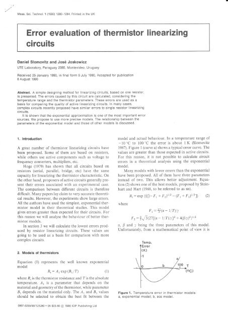
model and actual behaviour. In a temperature range of
-10"C to 100"C the error is about 1K (Slomovitz
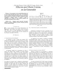
1987). Figure 1 (curve a) shows a typical error curve. The
values are greater than those expected in active circuits.
For this reason, it is not possible to calculate circuit
errors in a theoretical analysis using the exponential
model.
Many models with lower errors than the exponential
have been proposed. All of them have three parameters
instead of two. This allows better adjustment. Equation
(2) shows one of the best models, proposed by Steinhart
and Hart (1968, to be referred to as sri).
where
R, : exp {+t(- F, + F )tt3 - (F, + Fr)t/tl} (2)
F,:T@* llDlv
F, : 1 ú{27 1@ - r l r)lyl', + 4(p lú3}t t2
a, B and y being the three parameters of this model.
Unfortunately, from a mathematical point of view it is
Temp.
Error
(K)
T
(oc)
Figure 1. Temperature error in thermistor models:
a, exponential model; b, ees model.
0957-02331901121280+05 $03.50 @ 1990 IOP Publishing Ltd

Thermistor linearizing circuits
very cumbersome. Bosson et al (1950, to be referred to
as ncs) have proposed another model with similar errors
to the sn model for the temperature range - 10 "C to
100 "C. When a large range is used (-60 "C to 150'C)
the error of the scs model is three times greater than the
sH one. However, we prefer to use the ncs model, because
the mathematical expression (equation (3)) is simpler
than sH. This is an important advantage in theoretical
studies.
R,: Az exp lBrl(T + 0)1. (3)
The Ar, 82 and 0 parameters must be selected so as to
fit the experimental Rt(T) curve as well as possible. A
comparison of the error produced by these models in 13
different thermistors has been shown by Slomovitz
(1987). The scs model produces errors 10 to 20 times
smaller than the exponential model. A typical error curve
is shown in figure 1 (curve b).
The complexity of a theoretical study is increased
when a three-parameter model is used. Nevertheless, the
BGS parameters are not totally independent. A strong
correlation between B, and I was observed when these
parameters were calculated for the 13 thermistors previously
mentioned. Figure 2 shows that this relationship
can be approximated by a straight line. The best straight
line is
0:0.017982- 42.7 (4)
where 0 and B, are expressed in K. The standard deviation
is 12%. This reduces the number of independent
variables to two. Thus, studies using this model will not
be more complicated than those using the exponential
model.
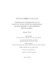
The parameter B, of the exponential model is related
to the parameter 82 of the scs model. Figure 3 shows
that when B, increases, B, also increases linearly. The
points in this figure were calculated using data from the
13 previously mentioned thermistors. The best straight
line for these points is given by using
Bz:23328r- 3268. (5)
Figure 3. Relationship between the parameters 8, (ecs
model) and 8, (exponential model).
In this way, it is possible to estimate the values of B, and
0 from the value of Br. using equations (4) and (5). We
will make use of this in section 4.
3. Single resistor linearizing circuit
Figure 4 shows one of the simplest linearizing circuits. U
is a constant voltage, Z" the output voltage, R, is the
thermistor and R is a resistor.
4: u l{:(AzlR)exp lB'lQ + 0)l + U. (6)
Figure 5 shows the relationship between V" and T.
We define the relative-temperature error E, as the percentage
temperature difference between the curve and the
straight line (100 x (segment GH/Q). Q is given in kelvin.
It is necessary, in the temperature range considered,
to choose the value of R, and to select the straight line
that fits the curve best, to reduce errors to a minimum.
Boél e/ al (1965) have proposed choosing the tangent
to the curve at the inflection point (corresponding to ft,),
as the straight line. This should produce errors similar
to those shown in figure 6, curve a. The value Q, is
imposed in the middle of the temperature range by Boél
82(K)
Figure 2. Relationship between the BGS parameters 0
and 8".
Figure 4. Resistive linearizing circuit of thermistors:
U, constant voltage; l/", output voltage.
1281

D Slomovitz and J Joskowicz
Tg To
Figure 5. Typical curve of output voltage V. versus the
thermistor temperature. Io is ihe temperature
corresponding to the inflection point.
Figure 6, Temperature errors according to different
designing methods: a, straight line tangent in the inflection
point; b, straight line passing through the extremes points;
c, straight line passing through Io with a slope between
cases a and b.
et al.This leads to a condition for the value of R. Using
the scs model, this condition is
Rr: Az exp lBrl(To + 0))
x lBz- 2(To+ e)lllBr+ 2(To+ 0)f (7)
Where Rr is the value of R calculated by this method.
Beakley (1951) proposed using the straight line that
passes through the two extreme points of the curve. The
shape ofthe curve should be ofthe type shown in figure 6,
curve b. He proposed choosing the R value according to
(7)
Khan (1985) mentioned that smaller errors could be
obtained using a straight line that passes through the
inflection point, with a slope slightiy smaller than the
tangent. The shape of the error curve should be similar
to curve c in figure 6. However, he did not show how to
choose this slope.
In all these cases, it was a condition that the inflection
point of the curve was in the centre of the temperature
range, and that the straight line passed through it. However,
there is no theoretical reason to support this. We
will show later that other criteria lead to smaller errors.
The analytical determination of the R value and the
best straight line for an optimal linearization is very cumbersome.
These parameters depend on Ar, Br, 0 and the
temperature range. We use a numerical method to solve
this problem. The maximum value of E. was used as the
quality parameter. However, in the other papers the
absolute temperature difference E, (segment GH in
figure 5) is used as the temperature error. For comparison
with these other papers, our results are expressed as
E,, in kelvin.
It was supposed that equation (3) represented exactly
the thermistor behaviour. The temperature difference h
(h: [,"*i^u- - 4n,n,-u-) of the considered range, was
varied between 50 K and 200 K. The thermistor parameters
were varied in the following ranges: Bt between
3000 K and 8000 K, and 0 +20% around the value given
by equation (4). R is proportional to the parameter Ar,
so it is not necessary to take into account the variation
of Ar. A change in the value of A, only produces a
proportional change in the value of R.
The circuit analysed has three variables. They are R,
and the two parameters that define the straight line. For
these two parameters, we used two of the intersection
points between the curve and the straight line (E and F
in figure 5). The calculating program varies these three
variabies, and selects the best values. This method usually
uses a lot of computer time, but in this case we know
approximately where the solution is. The two intersection
points are near the extremes of the temperature
interval and the value of R has the same order as the
value given by equation (7).
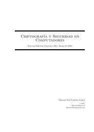
The error E, depends on the temperature difference
h, but it does not depend on where the range is. Figure 7
shows that different ranges lead to similar errors if h is
constant. In this figure, the abscissa represents the central
temperature f"(.7": (7."- + T^,^)12), and the ordinate the
calculated error E,. The circles correspond to a thermistor
for which Br:3000 K, the crosses to Bt:5000 K
and the triangles I"o 82:8000 K. In all these cases, the
value of I has been calculated according to equation (4).
The variation of 0 in a range of -12006 from the
central value given by (4), does not alter the errors in
practice. Figure 8 shows the variation of the error E,
against the ratio 0100, 0o being the value given by
equation (4). Thermistors with three different values of
Figure 7. lnfluence of the central temperature f on the
error E,. The temperature difference h is 150 K for all the
points. Circles, Ar:3000 K; crosses, 8r: 5000 K; triangles,
Az: 8000 K. The value of 0 is given by equation (4).
1282

Thermistor linearizing circuits
4. Error comparison with proposed linearizing circuits
Figure 8. lnfluence ot 0l0o on the error fi, 0o being the
calculated value according to equation (4).
1
Brwere used (circles, Bz : 3000 K; crosses, Br : 5000 K;
triangles, Bz : 8000 K). E, varies less than 14oA tn all
these cases. The temperature range was 0'C to 100'C
for all the points.
Accordingly, errors corresponding to different
methods are shown only as a function of h and 82. All
the temperature ranges begin at 0'C.
A large number of cases were studied using the
numerical method. From the results, a simple heuristic
designing method is proposed. This new method is very
simple to use. We suggest choosing the value of R according
to the heuristic equation
R: kRf (8)
where /r : 0.00313h + 0.913. k varies between 1.07 for h:
50K and 1.54 for h:200 K. As the straight line, we
propose choosing one that produces null errors at temperatures
correspondingto 6.90/o and 89.5oh of h. As an
example, consider a - 10 'C to 80 "C range. The value
of h is 90 K. There should be null errors at - 3.8 'C
(- 10 + 0.069 x 90) and 70.6 "C (- 10 + 0.895 x 90).
A comparison between the three methods mentioned
is presented in table 1. The proposed method (column 6)
has errors which are three times smaller than the Boél
method shown in column 4, and 1.6 times lower than the
Beakley method shown in column 5. On the other hand,
the average error of the proposed method is only 1.09
times greater than the errors generated by the numerical
method (column 7).
All authors, at present, have used the exponential thermistor
model in their analyses. To compare their results
against the proposed circuit. it is necessary to estimate
B, and 0 from the value Br. For this purpose, we will
use equations (4) and (5).
Sundqvist (1983) proposed a voltage to frequency
converter. According to his theoretical analysis, based on
the exponential model, the error should be zero. Nevertheless,
in his experimental results, errors as large as 2 K
appear in a 100 K range. These errors are attributed to
model errors. The thermistor used had Bt: 3725 K. This
is approximately equivalent to Bz:5420K. From
table 1 it is concluded that the error ofa resistive linearizing
circuit should be around 3.6 K. This error is of a
similar order to the active circuit error. This confirms
that the exponential model must not be used with active
circuits. Otherwise, the errors should be smaller than
those produced by resistive linearizing circuits.
Patranabis et al (1988) proposed using an active circuit
based on a logarithmic amplifier. They showed
errors around 1 K in the range 30'C to 95 'C. (They did
not show the thermistor value of Bt.) Using a resistive
circuit the error should be between 1 K and 2 K,
depending on the thermistor (see table 1). This shows
that just a single resistor is equivalent to a complex circuit,
so the usefulness of the circuit is doubtful.
Sengupta (1988) proposed a temperature to frequency
converter. His experimental results show errors of 0.7 K
in a range of 5'C to 85 "C. The thermistor used had
Br : 3400 K, corresponding to 82:4600 K. Table 1
shows that a resistive circuit has errors of around 2 K
for the same conditions. For applications where this
slightly higher error is acceptable, the resistive circuit
offers a much more cost-effective solution than the active
circuit.
On the other hand, Cole (1957)used a resistive circuit.
During the experimental work, he empirically adjusted
the resistor values and the straight line to obtain the
smallest error. The range considered was 2"C to 48 "C.
He imposed null errors at 5'C and 45 "C. These values
Table 1.
82 Range
(K) (K)
h
(K)
Method 1 Method 2 Method 3
E (K) E (K) E (K)
(Boél) (Beakley) (proposed)
Numerical
method
E. (K)
3000
3000
3000
3000
273-323
273-373
273-423
273-473
50
100
150
200
1.3
7.5
17.8
29.2
0.6
4.2
10.6
15.4
0.4
2.5
6.3
12.3
0.3
2.3
5.9
9.9
5000
5000
5000
5000
273-323
273-373
273-423
273-473
50
100
150
200
2.2
11.9
28.8
51.6
1.0
o.ó
15.7
26.8
0.6
3.6
9.3
17.5
0.6
3.6
8.5
16.1
8000
8000
8000
8000
273-323
273-373
273-423
273-473
50
100
150
200
3.0
16.4
38.9
68.1
1.4
8.2
20.3
35.4
0.9
4.8
12.2
22.7
0.9
4.8
11.0
20.8
1 283

D Slomovitz and J Joskowicz
are very close to those recommended for the proposed
method (5 "C and 43'C). The thermistor used had Bt :
3463 K, corresponding to 82 : 4800 K. The error
obtained, -E,, by Cole was 0.7 K. Table 1 forecasts 0.6 K.
This shows that the theoretical errors shown in table 1,
column 6, can be obtained in real experiments.
5. Conclusions
A method for designing resistive linearizing circuits has
been proposed. It is based on a three-parumeter thermistor
model (Bosson et aI 1950). Analysis of this model
shows that there is a strong correlation between the parameters.
Also, simple equations relate these parameters
to the exponential model parameters.
An error comparison between the proposed method
and active circuits was done. It is surprising that a lot of
recent papers show errors of the same order as those
produced by single resistor circuits. The principal cause
is that all of them are based on the simple exponential
approximation. For this reason they cannot be expected
to be perfect.
We propose using the results of this paper as a basis
for comparison of the quality of active linearizing
circuits.
References
Beakley W R 1951 The design of thermistor thermometers
with linear calibration J. Sci. Instrum.2S 176-9
Boé1 M and Erickson B 1965 Correlation study of a
thermistor thermometer Reu. Scí. Instrum. 36 904-8
Bosson G, Gutmann F and Simmons L M 1950 A
relationship between resistance and temperature of
thermistors J. Appl. Phys.21 1267-8
Cole K S 1957 Thermistor thermometer bridge: linearity and
sensitivity for a range of temperature Reu. Sci. InsÚum.
28 326-8
Hoge H J 1979 Comparison of circuits for linearizing the
temperature indications of thermistors Reu. Sci. Instrum.
s0 316-20
Khan A A 1985 Linearization of thermistor thermometer Inú.
J. Electron.59 129 39
Patranabis D, Ghosh S and Bakshi C 1988 Linearizing
transducer characteristics IEEE Trans. Instrum. Meas.37
66-9
Sengupta R N 1988 A widely linear temperature to frequency
converter using a thermistor in a pulse generator IEEE
Trans. Instum. Meas.37 62-5
Slomovitz D 1987 The temperature/resistance curve of NTC
thermistors Test and Measurement World 7 (5) 73-9
Steinhart J S and Hart S R 1968 Calibration curves for
thermistors Deep-Sea Res. 15 497-503
Sundqvist B 1983 Simple, wide-range, linear temperature-tofrequency
conve¡ters using standard thermistors J. Phys.
E: Sci. Instrum. 16 261-4
1284